iLogic in Autodesk Inventor [5]). ...... commercial 3D CAD system (Autodesk Inventor) used to create the ...... DFT file, to store NC commands and tooling.
Automatic Assembly-Model Synthesis in Mechanical Design using Simulated Dynamic Finite-Element Experiments
Doctoral Thesis by
Iraklis Chatziparasidis
University of Western Macedonia Faculty of Engineering Department of Mechanical Engineering
June 2017
Automatic Assembly-Model Synthesis in Mechanical Design using Simulated Dynamic Finite-Element Experiments
Doctoral Thesis by
Iraklis Chatziparasidis Thesis submitted in partial fulfilment of the requirements of the Degree of Doctor of Philosophy
Advisory Committee: Supervisor: Nickolas S. Sapidis Professor Department of Mechanical Engineering University of Western Macedonia Members:
Georgios Andreadis Associate Professor Department of Mechanical Engineering Aristotle University of Thessaloniki Dimitrios Giagopoulos Assistant Professor Department of Mechanical Engineering University of Western Macedonia
Automatic Assembly-Model Synthesis in Mechanical Design using Simulated Dynamic Finite-Element Experiments Doctoral Thesis by
Iraklis Chatziparasidis Examination Committee
Nickolas S. Sapidis Professor Department of Mechanical Engineering University of Western Macedonia
Georgios Andreadis Associate Professor Dept. of Mechanical Engineering Aristotle University of Thessaloniki
Dimitrios Giagopoulos Assistant Professor Dept. of Mechanical Engineering University of Western Macedonia
Nikolaos Bilalis Professor School of Production Engineering and Management Technical University of Crete
Philip Azariadis Associate Professor Dept. of Product & Systems Design Engineering University of the Aegean
Georgios Maliaris Assistant Professor Dept. of Electrical and Computer Engineering Democritus University of Thrace
Panagiotis Kyratsis Assistant Professor Dept. of Mechanical Engineering & Industrial Design Western Macedonia University of Applied Sciences
To : my wife Fotini my son Morpheus my daughter Hero
Acknowledgements First, I would like to express my sincere gratitude to my supervisor, Professor Nickolas S. Sapidis for giving me the opportunity to pursue a Doctoral Degree. I would like to thank him for his continual effort to teach me how a Researcher must think, work and write. I know that this was not an easy task. He literally transformed my way of thinking and this is a present that I will always bring with me. I would like to express my sincere gratitude to Assistant Professor Dimitrios Giagopoulos. All these years we have worked very close together. I have learned many things and it is always a pleasure to work with him. His contribution to this thesis was invaluable. I would like to thank Associate Professor Georgios Andreadis, the discussions with him were always essential and useful. His big experience and deep knowledge in CAD systems was invaluable. I would like to thank Konstantinos Liaretidis, Technical Director at Kleemann Hellas SA, for supporting me in pursuing my PhD degree while I was working fulltime in industry. Working with Konstantinos Liaretidis is always pleasant. Finally, I would like to give my special thanks to Ioannis Sanidiotis, Deputy General Manager at Kleemann Hellas SA. He was extremely supportive from the begging. A big part of my Doctoral Research is now a fully functional Design Automation application just because of his support.
i
Abstract Today, in the context of a globalized market, customers have high demands for products that are tailored to their individual needs and are offered at a price that is very close to that of massproduced products. Engineering-To-Order (ETO) companies are forced to reduce costs and lead time to gain an advantage over the competition. These companies encounter two major issues that greatly affect the cost and the quality of their products. The first issue is the configuration complexity of ETO products. Many ETO companies are employing Knowledge Based Engineering (KBE) systems to manage the configuration complexity. These systems can be used to effectively capture knowledge by storing technical guidelines, "best practices", and even a company’s commercial and business rules. When it comes to complicated product configurations, the use of KBE tools is indeed an efficient solution automating configuration specification. However, ETO companies very often are confronted with "first-time" product configuration requirements. Since previous experience design rules are not adequate to cover the new configuration requirements, these companies are usually proceeding with experimental tests using full scale prototypes to check the structural integrity of the proposed design, spending time and raw materials. Also, since these tests must be performed, usually, in very tight lead times required by the customer, the design/engineering team has very limited time to achieve optimized material usage, reduced weight, etc. Thus, usually they end up with over-engineered solutions. ETO companies could gain significant benefits and achieve significant cost reduction if they could perform simulated experiments using Finite Elements Analysis models instead of using full scale prototypes. A major concern about using FE simulated experiments is the validation of the FE models in terms of their accuracy. FE model validation is even more complicated to be achieved for dynamic phenomena simulations. The second issue is the time and the cost required for the product to be designed and engineered, and for manufacturing drawings to be published and launched to the shop floor. In most cases, these companies have a number of premade 3D models (and the corresponding manufacturing drawings) and modify them to adjust the dimensions, the function and/or the aesthetics of the product to the customer requirements. Unfortunately, this method is prone to human errors, and these errors may create extra remanufacturing costs. An ETO company would gain a significant advantage by using a tool that would create automatically 3D assembly models for its products. In this thesis a framework that addresses both of these issues is presented. The present framework provides: a) usage of FE models and simulated dynamic experiments to deduce new design rules, instead of performing experiments with full scale prototypes, b) a methodology for
ii
validating these finite element models for their accuracy in simulating dynamic experiments and c) a Mechanical-Design methodology based on the Automatic Assembly Synthesis Model (AASM), that links a KBE and a CAD system, and automatically generates and synthesizes the final 3D assembly model.
Keywords: Design Automation; Automatic Assembly Synthesis; Assembly Features; Assembly Model; Routine Design.
iii
Contents Acknowledgements ............................................................................................................................. i Abstract .............................................................................................................................................. ii List of Acronyms ................................................................................................................................ vi List of Figures ................................................................................................................................... vii List of Tables ...................................................................................................................................... xi 1
Introduction ............................................................................................................................... 1
2
Literature Review ....................................................................................................................... 4 2.1
Verification and Validation of Simulation Models ..........................................................4
2.1.1
3
2.2
Class of Mechanical Systems – Equations of Motion ......................................................8
2.3
Finite Element Model Updating Methods .......................................................................9
2.4
Design Automation........................................................................................................11
2.4.1
Assembly Modelling & Product Architecture ....................................................... 11
2.4.2
Top-Down & Skeleton-based Design .................................................................... 12
2.4.3
Assembly Features ............................................................................................... 12
The Automatic Mechanical-Design Methodology.................................................................... 15 3.1
Finite-Element Simulation Models for Dynamic Mechanical Systems ..........................15
3.2
The Simulated Dynamic Experiment Validation Method (SEVaM) ...............................15
3.3
Design Rules and Product Configuration.......................................................................16
3.4
The Automatic Assembly Synthesis Model (AASM) ......................................................17
3.4.1
“Half” Assembly Constraints ................................................................................ 18
3.4.2
Assembly Feature (AF): A New Definition for the Automatic Assembly Synthesis
Model
4
Verification & Validation: Definitions and Models................................................. 4
.............................................................................................................................. 19
3.4.3
AASM: The Schematic Assembly Model (SAM) .................................................... 22
3.4.4
AASM: The Intermediate Assembly Model (IAM) ................................................ 27
The Comprehensive Mechanical-Design Framework............................................................... 36 4.1
Application of SEVaM to a Passenger Elevator System.................................................37
4.1.1
Analysis of the Sling .............................................................................................. 41 iv
4.1.2 4.2
Analysis of the Complete Elevator System ........................................................... 55
Implementation of SEVaM in a Full Glass Panoramic Elevator System ........................57
4.2.1
Validation of a Glass Panel with Suspension Components FE Model .................. 57
4.2.2
FE model parameterization and Updating Results............................................... 61
4.2.3
Static Tension Load FE Model and Experimental Results..................................... 63
4.2.4
Analysis of the FE Model of the Full Elevator System with a Frameless Full Glass
Car
.............................................................................................................................. 65
4.3
Design Rules Deduced from Simulated Experiments ....................................................72
4.4
Implementation of the Automatic Assembly Synthesis Model (AASM) .......................74
5
Conclusions and Discussion...................................................................................................... 80
6
Future Work ............................................................................................................................. 82
Appendix - Published Papers ............................................................................................................ 93 P1.
Framework to Automate Mechanical-System Design using Multiple Product-Models
and Assembly Feature Technology ...............................................................................................93 Abstract ............................................................................................................................................ 93 P2.
Automatic Assembly Design for Engineering-To-Order Products based on Multiple
Models and Assembly Features ....................................................................................................94 Abstract ............................................................................................................................................ 94 P3.
Optimum Design, Finite Element Model Updating and Dynamic Analysis of a Full
Laminated Glass Panoramic Car Elevator .....................................................................................95 Abstract ............................................................................................................................................ 95 P4.
Optimum Design and Dynamic Analysis of a Full Glass Panoramic Car Elevator
Through Finite Element Modeling and Experimental Tests ..........................................................96 Abstract ............................................................................................................................................ 96 P5.
Structural integrity analysis and optimization of an elevator frame, through FE
modeling and experimental tests .................................................................................................97 Abstract ............................................................................................................................................ 97
v
List of Acronyms AASM
Automatic Assembly Synthesis Model
AF
Assembly Feature
AFA
Assembly Feature Association
AFAP
Assembly Feature Attribute Pair
AFAPA
Assembly Feature Attribute Pair Association
CAD
Computer Aided Design
CAE
Computer Aided Engineering
DA
Design Automation
ETO
Engineering-To-Order
FEA
Finite Element Analysis
FRF
Frequency Response Function
GRMS
Root Mean Square of Acceleration (g)
IAM
Intermediate Assembly Model
KBE
Knowledge Based Engineering
SAM
Schematic Assembly Model
SEVaM
Simulated Experiments Evaluation Method
vi
List of Figures Fig. 1 – Finite Element Simulated Experiments for Design Rules Deduction
3
Fig. 2 - Confidence that model is valid [16]
5
Fig. 3 - Simplified version of the model development process [16]
6
Fig. 4 - Verification in digital and physical world [12]
7
Fig. 5 - The Simulated Experiment Validation Method (SEVaM)
16
Fig. 6. AASM Model
17
Fig. 7. Automatic Assembly Synthesis Work Flow
18
Fig. 8. Assembly Features and Assembly Features Pairs
20
Fig. 9. Skeleton Assembly Feature to Simulate Spot Welding Connection
21
Fig. 10. External Assembly Feature
22
Fig. 11. The Schematic Assembly Model consists of the SAM_Structure and the SAM_Connection Rules Collection
24
Fig. 12. Left & Right Sling Elevator
26
Fig. 13. Left & Right Sling Elevator Roofs
26
Fig. 14. Step 1: IAM initialization
27
Fig. 15. SAM Component - IAM Component and 3D Part Model Association
28
Fig. 16. Step 2: Generation of 3D Part Models
29
Fig. 17. AF Association
30
Fig. 18. Step 4: IAM and SAM Compatibility Check
32
Fig. 19. Step 4: AF Association Validated
33
Fig. 20 - Multiple IAM implementations for the same SAM
34
Fig. 21 - Appended SAM - IAM
35
Fig. 22 - Comprehensive Mechanical-Design Framework
36
Fig. 23 - (a) Elevator’s sling, (b) Elevator’s Car
37
Fig. 24 - Finite element model of the sling with car
38
Fig. 25 - Overspeed Governor Device
39
Fig. 26 - Overspeed Governor System
39
vii
Fig. 27 - Slide catch component
40
Fig. 28 - Triggering shaft
40
Fig. 29 - Finite element model of the elevator sling including the platform of the car with full load
42
Fig. 30 - First, Second and Fifth eigenmodes of the sling predicted by the FE Model
42
Fig. 31 - Measurement locations of acceleration time histories
43
Fig. 32 - (a) Experimental device, (b) Data acquisition system, and (c) Elevator platform with load
44
Fig. 33 - Acceleration measurement locations at a connection point (A1) and at a reference point (A4)
44
Fig. 34 - Acceleration time histories in the: (a) x-longitudinal direction, (b) y- vertical direction and (c) ztransverse direction, with peak to peak and GRMS values for Case A Fig. 35 - High Speed Camera
45 46
Fig. 36 - Comparison of maximum-displacement estimations based on the experiment (high-speed camera) and on numerical calculation (dynamic finite element analysis)
47
Fig. 37 - Comparison of experimentally measured (continuous lines) and numerically determined (broken lines) accelerations at two indicative locations (A3 and A4) of the sling, in the vertical direction
47
Fig. 38 - Locations of the sling where maximum stresses appear
48
Fig. 39 - Measurements locations where maximum stress appears
48
Fig. 40 - Strain gauges measurement locations
49
Fig. 41 - Equivalent (von Mises) stress histories, together with the maximum value of this stress, measured at the locations (SG1 - SG4) during one of the tests (PG3) for Case A
50
Fig. 42 - Maximum values of the von Mises stress, calculated by the finite element model analysis at the locations (SG1 - SG4) for Case A
51
Fig. 43 - Acceleration time histories in the: (a) x-longitudinal direction, (b) y- vertical direction and (c) ztransverse direction, with peak to peak and GRMS values for Case B
52
Fig. 44 - Comparison of maximum-displacement estimations for the free fall test, based on the experiment (photo) and on numerical calculation (: dynamic finite element analysis) for Case B
53
Fig. 45 - Equivalent (von Mises) stress histories, together with the maximum value of this stress, measured at the locations (SG1 - SG4) during one of the tests, for Case B
54
Fig. 46 - Maximum values of the von Mises stress, calculated by the finite element model analysis at the locations (SG1 - SG4), for Case B
54
viii
Fig. 47 - Experimental set up of the complete elevator system
55
Fig. 48 - Locations of the elevator system where maximum stresses appear and comparison with experimental results
56
Fig. 49 - Finite Element Model of the Glass Panel with Support
58
Fig. 50 - Typical Eigenmodes Predicted by the Nominal Finite Element Mode
58
Fig. 51 - Schematic Illustration of the Experimental Device, Fixed-Free Arrangement with Electrodynamic Shaker, Accelerometers and Strain Gauges Locations
59
Fig. 52 - Typical Elements of the FRF Matrix
60
Fig. 53 - Parts of the Parameterized FE Model
61
Fig. 54 - Comparison between measured, nominal and optimal acceleration time histories and FRF at the location A1
63
Fig. 55 - Tension Load Test Simulation Results
64
Fig. 56 - Tension Load Experiments
64
Fig. 57 - Frameless Full Glass Car FE model
65
Fig. 58 - High Stresses Locations in the Glass Components and Strain Gauges Placement
66
Fig. 59 - Full Glass Frameless Car Experimental Verification Set Up
67
Fig. 60 - Stain Gauges on Selected Location on the Glass Components
68
Fig. 61 - Experimental Acceleration Values on Glass Components
69
Fig. 62 - Numerical and Experimental Stress values Comparison on the Upper Locations
69
Fig. 63 - Numerical and Experimental Stress values Comparison on the Lower Locations
70
Fig. 64 - Full Glass Frameless Car
71
Fig. 65 - Car Roof Experimental Model
72
Fig. 66 - Car Roof 3D model
73
Fig. 67 - Parametric Drawings Recording the Design Rules Deduced from Simulated Experiments
73
Fig. 68 - Car Roof Design Rules
74
Fig. 69. Examples of AFs
75
Fig. 70. User Interface of CabinsKBE (: the CAD add-in Implementing AASM)
77
Fig. 71. A Panoramic Elevator Car Automatically Generated and Synthesized by CabinsKBE
78
Fig. 72. A Passenger Elevator Car Automatically Generated and Synthesized by CabinsKBE
78
ix
Fig. 73 - Descriptive XML Language for Product Configuration and SAM Automatic Development
83
Fig. 74 - Optimized ETO Solution Loop
84
x
List of Tables Table 1 - Assembly Semi-Constraints
21
Table 2 - Kinematic Pairs
25
Table 3 - Kinematic Pairs and implementations using AFAPs
31
Table 4 - Maximum Value of Equivalent Stress von Mises [Mpa]
49
Table 5 - Modal Frequencies and Modal Damping Ratios
60
Table 6 - Design Variables and Optimization Design Limits
62
Table 7 - Comparison Between Identified and Optimal FE Predicted Modal Frequencies
62
Table 8 - Comparison Between FE model and Experimental Results in Tension Load Tests
65
xi
1 Introduction Today, in the context of a globalized market, customers have high demands for products that are tailored to their individual needs and are offered at a price that is very close to that of massproduced products. Companies producing Engineering-To-Order products are forced to reduce costs and lead time to gain a competitive advantage over competition. To deal with ETO product configuration complexity, many ETO companies are using Knowledge Based Engineering systems (KBE). These systems can be employed to effectively capture knowledge by storing technical guidelines, relations, facts [1], "best practices", and even a company’s commercial and business rules. However when a "first-time" product configuration requirement occurs, the KBE system does not contain any adequate rules based on previous experience. In such cases, companies spend time and raw materials for full-scale structural integrity tests. Usually, these tests must be performed in very tight deadlines required by the customer, leaving to the design/engineering team very limited time to achieve optimized material usage, reduced weight, etc. Thus, usually they end up with over-engineered solutions. ETO companies could gain significant benefits and achieve significant cost reduction if they could perform simulated experiments using Finite Elements Analysis models instead of using full scale prototypes. A major concern about using FE simulated experiments is the validation of the FE models in terms of their accuracy. FE model validation is even more complicated to be achieved for dynamic phenomena simulations. Another major cost factor for ETO companies is the time required for the product to be designed and for manufacturing drawings to be published and launched to the shop floor. In most cases, these companies have a number of premade 3D models (and the corresponding manufacturing drawings) and modify them to adjust the dimensions, the function and/or the aesthetics of the product to the customer requirements. Unfortunately, this method is prone to human errors, and these errors may create extra remanufacturing costs. An ETO company would gain a significant advantage by using a tool that would create automatically 3D assembly models for its products. Today, CAD systems can be used to partially automate some routine design operations when these are combined with generative modelling methodologies [2,3]. Most modern CAD systems either provide programming capabilities [4] that allow some tasks to be automated, or they have embedded tools that can be used to create generative models (e.g., iLogic in Autodesk Inventor [5]). These tools can record expert knowledge in the form of "IF…THEN…ELSE" rules. These rules are used to control the geometry of components, their properties, and/or participation of a component into an assembly. However, this kind of tools can be used only in situations where all configurations in the final product are known. Often this is
1
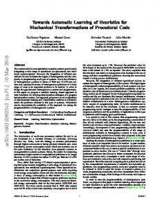
not true, as many ETO companies prefer more flexible approaches to product configuration, employing Knowledge Based Engineering systems (KBE). These systems can be used to effectively capture knowledge by storing technical guidelines, relations, facts [1], "best practices", and even a company’s commercial and business rules. When it comes to complicated product configurations, the use of KBE tools is indeed an efficient solution automating configuration specification. However, on the side of CAD systems a major limitation remains: it is extremely difficult to have pre-defined 3D assembly models matching all possible product configurations implied by a KBE system. The first contribution of this dissertation (Chapter 3) is development of a novel approach to "routine design" automation that transforms KBE instructions (defining a Product Configuration) into a fully-detailed 3D assembly model, created from scratch by synthesizing appropriate components. Since existing assembly modelling methods are not well suited for design automation procedures, this work presents the Automatic Assembly Synthesis Model (AASM), a model/method to link a KBE and a CAD system. This model makes possible development of design automation applications for 3D assembly models without use of predefined 3D assembly master models. To facilitate the connection between a KBE and a CAD system, AASM contains a dual representation of the product. The first representation is modelling the KBE requirements in a “neutral” object-oriented model, named as Schematic Assembly Model (SAM). The second representation, named as Intermediate Assembly Model (IAM), is describing a CAD implementation of the given SAM. AASM also provides the means to implement generic connection descriptions, implied by the SAM, into fully kinematic relations between components in the final 3D assembly model. To achieve this, AASM uses the concept of Assembly Features (AFs). In this work a new definition of Assembly Features is presented. Here, AFs are redefined and incorporated within AASM in a way that facilitates the communication between a KBE and a CAD system. They are structured in an object-oriented manner and constitute the means by which automatic connection of 3D component models is achieved. Finally the dual-representation structure of AASM provides the ability to have more than one IAM implementations for the same SAM. This offers the ability to materialize multiple 3D models implementing the same product configuration and choose the solution presenting the best performance in terms of e.g. weight, cost, lead time, number of components, etc. The second contribution of this dissertation (Chapters 3 & 4) focuses on a comprehensive mechanical-design framework (Fig. 1) where finite element (FE) models are used to simulate experiments, modelling newly defined product configurations. The results of these simulated experiments are then used to deduce new design rules that are passed to the KBE system. The Simulated Experiment Validation Method (SEVaM) used for the validation of the FE models is also 2
presented. SEVaM provides a mixed computational-experimental method aiming to the estimation of the stresses developed on dynamic mechanical systems. SEVaM uses experimental results as input in the simulation models and contains procedures allowing the simulation model to be calibrated to given experimental results. The product configuration from the KBE system is then passed to a custom developed CAD application, based on the Automatic Assembly Synthesis Model (AASM) and Assembly Features [6,7], that automatically generates all the 3D CAD components and synthesizes the final 3D CAD assembly model.
Fig. 1 – Finite Element Simulated Experiments for Design Rules Deduction
3
2 Literature Review 2.1 Verification and Validation of Simulation Models A simulation model provides about the only method to study new, non-existent complex dynamic systems and it is a powerful tool for the analysis of new system designs
[8]. In
simulation, we study real dynamic systems, how they change over time and how subsystems and components interact [8,9]. Simulation-based design is a process in which simulation is the primary means of design evaluation and verification. When coupled with appropriate validation processes executed during the development of a simulation-based design system, the resulting capabilities can provide companies the ability to design superior products in less time and at lower costs. The application of simulation-based design is used in situations where the cost associated with the application of the classic methods of prototype construction and test is prohibitively time consuming and expensive [10]. Model validation is an important aspect of any model-based methodology in general, and system dynamics in particular [11]. When it comes to engineering designs, the verification and validation are of primary importance as they directly influence production performance and ultimately define product functionality [12]. A verified and validated model implies its reliability as a basis for decision-making [13].
2.1.1 Verification & Validation: Definitions and Models According to [14], Verification is the process of ensuring that the model is built right. Validation, on the other hand, is the process of ensuring that the model is sufficiently accurate. A key concept is the idea of sufficient accuracy. No model is ever 100% accurate. The aim of Verification & Validation is to ensure that the model is sufficiently accurate and it is seen as a process of increasing confidence in a model, and not one of demonstrating absolute accuracy. A simulation model of a complex system can only be an approximation to the actual system, no matter how much time and money is spent on model building. Indeed, a model is supposed to be an abstraction and simplification of reality. The more time (and hence money) that is spent on model development the more valid the model should be in general. However, the most valid model is not necessarily the most cost-effective. For example, increasing the validity of the model beyond a certain level might be quite expensive, since extensive data collection may be required, but might not lead to significantly better insights or decisions [15]. Fig. 2 contains two relationship curves regarding confidence that a model is valid. The cost curve of performing model validation shows that cost increases at an increasing rate as the confidence in the model increases. The value curve shows that the value of a model to a user 4
increases as the confidence in the model increases but at a decreasing rate. The cost of model validation is usually quite significant, especially when extremely high model confidence is required [16].
Fig. 2 - Confidence that model is valid [16] The work [17] defines Verification as: The process of determining that a model implementation accurately represents the conceptual description of the model and the solution to the model, while model validation is the process of determining the degree to which a numerical model is an accurate representation of the real world from the perspective of the intended uses of the model. In [18], Verification is defined as: The process of determining if a computational model obtained by discretizing a mathematical model of a physical event and the code implementing the computational model can be used to represent the mathematical model of the event with sufficient accuracy. While Validation is defined as: The process of determining if a mathematical model of a physical event represents the actual physical event with sufficient accuracy. [14] proposes two phases of model Validation: a) White-box Validation and b) Black-box Validation. In White-box Validation one determines if the constituent parts of the computer model represent the corresponding real world elements with sufficient accuracy. In Black-box Validation one determines if the overall model represents the real world with sufficient accuracy. According to [15], the most definitive test of a simulation model’s validity is establishing that its output data closely resemble the output data that would be observed from the actual system. Since the scope of the present work is validation of FE dynamic analysis in mechanical systems, resembling the stresses measured on the actual system will be the means for the validation of the FE models. The work [16] presents the following model development process; see Fig. 3. The problem entity is the system to be modelled; the conceptual model is the mathematical / logical /graphical representation of the problem entity developed for a particular study; and the computerized model is the conceptual model implemented on a computer. Conceptual model validation is
5
defined as determining that the theories and assumptions underlying the conceptual model are correct and that the model representation of the problem entity is ‘reasonable’ for the intended purpose of the model. Computerized model verification is defined as assuring that the computer programming and implementation of the conceptual model are correct. Operational validation is defined as determining that the model’s output behaviour has a satisfactory range of accuracy for the model’s intended purpose over the domain of the model’s intended applicability. Data validity is defined as ensuring that the data necessary for model building, model evaluation and testing, and conducting the model experiments to solve the problem are adequate and correct.
Fig. 3 - Simplified version of the model development process [16] Maropoulos and Ceglarek in [12], present an excellent review of the standard definitions of verification and validation in the context of engineering design and progresses to provide a coherent analysis and classification of these activities from preliminary design, to design in the digital domain and the physical verification and validation of products and processes. Maropoulos and Ceglarek in [12] also present the verification model that is shown in Fig. 4 where a variety of design verification aspects are shown. However both models, presented by [16] and [12], do not specify a procedure for using experimental results as input in the simulation models. More specifically, in dynamic situations we have forces implied to the mechanical system that cause accelerations or/and decelerations. Also, stresses are caused both because of the forces and the accelerations/decelerations. These forces are unknown but they can be deduced by experimental measurements of the accelerations / decelerations. Also these models do not provide any FE 6
model adjusting procedure, like, e.g., the FE updating methods [19], to calibrate the simulation model to given experimental results.
Fig. 4 - Verification in digital and physical world [12]
7
Finally, it is noted that indeed many researchers discuss linking of a KBE with finite-element based structural analysis [20–26]. However, these works do not deal with the whole Mechanical Design process; they are aiming at using KBE systems only to automate creation of FE models.
2.2 Class of Mechanical Systems – Equations of Motion The equations of motion of mechanical systems with complex geometry are commonly set up by applying finite element techniques. Quite frequently, a systematic investigation of the dynamics of large scale mechanical structures leads to models involving an excessive number of degrees of freedom. Therefore, a computationally efficient solution requires application of methodologies reducing the numerical dimension of the original model [27–34]. Next, the basic steps of a time domain reduction method are presented briefly. For simplicity, consider a mechanical system consisting of two subsystems, say A and B. Moreover, let the equations of motion for subsystem A be derived from the following classical form
(1) where Mˆ A , Cˆ A and Kˆ A are, respectively, the mass, damping and stiffness matrix of the subsystem A, with the vector
fˆ
A
representing the external forcing. For a typical model, the
(t )
number of these equations may be quite large. However, for a given level of forcing frequencies, it is possible to reduce significantly the number of the original degrees of freedom, without sacrificing the accuracy in the numerical results, by applying standard component mode synthesis methods [29,31]. This can be achieved through an approximate coordinate transformation of the form
x A A q A
(2)
The transformation matrix A includes an appropriately chosen set of the lowest frequency normal modes of component A, corresponding to support-free conditions [29]. The number of these modes depends on the accuracy required in the response frequency range examined. Consequently, matrix A is completed by a set of static correction modes of component A [28,30]. Employing this transformation, the original set of equations (1) can be replaced by a considerably smaller set of equations, expressed in terms of the new generalized coordinates q A . More specifically, application of the Ritz transformation (2) onto the original set of equations (1) yields the much smaller dimension set
C A q K A q f (t ) M Aq A A A A
8
(3)
where ˆ , C T Cˆ , K T Kˆ and f M A AT M A A A A A A A A A A
A
AT fˆ A .
Moreover, the set of unknowns can be split in the form
qA (pA T
T
x b )T
where p A includes coordinates related to the response of internal degrees of freedom of component A, while x B includes the boundary points of component A with component B. Next, similar sets of equations of motion are obtained for component B. Namely, the equations of motion are first set up in the form
C B q K B q f (t ) MBq B B B B
(4)
with coordinates
qB ( pB T
T
x b )T
Then, a proper combination of equations (3) and (4) leads to the equations of motion of the composite system in the classical form C q K q f (t ) Mq
(5)
with coordinates
q ( pA T
T
pB
T
xb )T
The stiffness matrix of the composite system can be obtained by considering the total potential energy of the system. Likewise, the mass matrix of the composite system is obtained by considering the corresponding kinetic energy, while the forcing vector is determined by considering the virtual work.
2.3 Finite Element Model Updating Methods Let
ˆ r , ˆr R No , r 1, D {
, m}
be the measured modal data from a structure, consisting
of modal frequencies ˆ r and mode shape components ˆr at N o measured DOFs, where m is the number of observed modes. Consider a parameterized class of linear structural models used to model the dynamic behaviour of the structure and let R N be the set of free structural model parameters to be identified using the measured modal data. The objective in a modal-based structural identification methodology is to estimate the values of the parameter set so that the modal data {r ( ), r ( ) R N , r 1, , m} predicted by the linear class of models at the 0
9
corresponding N 0 measured DOFs best matches the experimentally obtained modal data in D . For this, let
2 ( ) ˆ r2 ( ) r ˆ r2
and r ( )
r
r ( )r ( ) ˆr
(6)
ˆr
be the measures of fit or residuals between the measured modal data and the model predicted modal data for the
r -th
modal frequency and mode shape components, respectively, where
|| z ||2 z T z is the usual Euclidean norm, and r ( ) ˆrT r ( ) / r ( )
2
is a normalization constant
that guaranties that the measured mode shape ˆr at the measured DOFs is closest to the model mode shape r ( )r ( ) predicted by the particular value of . To proceed with the model updating formulation, the measured modal properties are grouped into two groups. The first group contains the modal frequencies while the second group includes the mode shape components for all modes. For each group, a norm is introduced to measure the residuals of the difference between the measured values of the modal properties involved in the group and the corresponding modal values predicted from the model class for a particular value of the parameter set q . For the first group, the measure of fit J 1 ( q ) is selected to represent the difference between the measured and the model predicted frequencies for all modes. For the second group, the measure of fit J 2 ( q ) is selected to represent the difference between the measured and the model predicted mode shape components for all modes. Specifically, the two measures of fit are given by m
m
r 1
r 1
J 1 ( ) 2r ( ) and J 2 ( ) 2r ( )
(7)
The parameter estimation problem is traditionally solved by minimizing the single objective J ( q ; w) =
w1 J 1 ( q ) + w2 J 2 ( q )
(8)
formed by the two objectives J i ( q ) , using the weighting factors wi 0 , i = 1,2 , with w1 + w2 = 1 . The objective function J ( q ; w) represents an overall measure of fit between the
measured and the model predicted characteristics. The relative importance of the residual errors in the selection of the optimal model is reflected in the choice of the weights. The results of the identification depend on the weight values used. The optimal solutions for the parameter set for given w are denoted by ˆ( w) [33–35].
10
2.4 Design Automation In this thesis a model, supporting the automated assembly synthesis of 3D CAD models, is presented. This model is named as Automatic Assembly Synthesis Model (see Section 3.4), and it is based on concepts from various areas including feature-based design, product architecture, assembly modelling, top-down and skeleton design methods, design automation, with an emphasis on assembly features.
2.4.1 Assembly Modelling & Product Architecture According to [36], Assembly Modelling deals with the definition of an informational product model including all product components and the related relationship information. Being an informational product model definition, assembly modelling is used in: conceptual design, product data exchange, concurrent engineering and assembly planning. Many researchers have proposed different assembly models to achieve different goals. In [37], a multi-level assembly model is proposed to support collaborative top-down assembly design for geographically-dispersed designers. [38] proposes an assembly model, called AREP (Assembly REPresentation), using directed acyclic graphs to represent an assembly and relation graphs to describe relations between components, aiming at a lightweight assembly model adequate for collaboration via the internet. [39] introduces an integrated product model that incorporates a feature-based representation scheme for capturing product semantics, handled in the conceptual design phase, and links early design with part and assembly modelling. In [40], an integrated object-oriented product model for both single parts and assembly modelling and planning is introduced. In [41], a dual product model based on the Feature GraphTree Model (FGTM) is presented. The FGTM is comprised of the function model (FFGT) and the assembly model (AFGT). FFGT mainly records functional information while AFGT contains structural information. FGTM does not provide the information regarding how two components could be automatically connected and so it is not adequate for use in a design automation framework. However, the idea of having a dual assembly model, where structural elements are separated from other information (like connection rules), is indeed useful and it has been adopted also by the AASM model, proposed in the present dissertation. [42] present a data structure representing assemblies in a database divided into two parts. The first part is the data structure used to store topological and geometric information on each component in an assembly. The second part includes information on how components are placed into an assembly. [43] present a model for assembly sequence modelling, where the structural information is also separated from the geometrical information. [44] also use multiple graphs identifying functionally
11
similar assemblies. In [45], an object-oriented definition of an assembly model called the Open Assembly Model (OAM) is presented. The OAM represents the function, form, and behaviour of the assembly and defines both a system-level conceptual model and associated hierarchical relationships. The OAM includes sufficiently rich data structures to capture the assembly evolution from concept to detailed design. The OAM is a significant contribution and it greatly influenced also the present research. As this literature review makes clear that current assembly models are not adequate for automated assembly procedures, this dissertation focuses on exactly presenting an assembly model and methodology appropriate for automatic assembly synthesis for ETO products.
2.4.2 Top-Down & Skeleton-based Design Top-down approaches are mainly aimed at the initial phases of product design known as Conceptual Design. Top-down design is usually employed in combination with Skeleton Design techniques. A skeleton is a preliminary geometric description of parts or assembly, recording space and form restrictions to be used in the detail design phase [1,36,37,46–48]. At a later stage, the designer refines this skeleton by adding details that take under consideration relevant requirements posed by strength, cost, manufacturability, serviceability, and other considerations [49]. Top-down and Skeleton-based design methods are aimed at providing a common structure, space limits and connection interfaces between assembly components during the initial conceptdesign phase. In these methods, human interaction is a fundamental element. Also, these methods do not enable automated topological and geometrical alterations of the model. Thus, Top-down and Skeleton-based design methods are not adequate to support completely automated assembly synthesis in routine design tasks.
2.4.3 Assembly Features In feature-based product modelling, the Assembly Feature (AF) is an important concept describing relationships and interaction regions between parts, however, currently there is no unified definition for it [50]. In [40], an AF is defined as an information carrier for assemblyspecific information. In [41], an AF is defined as a pair of geometry features restricted by a specific assembly constraint. According to [51], an AF represents a region of a component that is of interest in the assembly context. In [45], an AF specifies relationships in a pair of assembled components. In [52], an AF is defined as an association between two form features which are on different parts. In [53], an AF is defined as a generic "solution" referring to two groups of parts
12
that need to be related by a relationship to solve a design problem. In [54], mating features are defined as those features that comprise mating relations between parts to be assembled. In [55,56], a method that simplifies complex products to achieve a virtual assembly modelling process in real time is presented. Here, form features are defined as generic shapes useful in computer-aided design applications, and assembly features are the connections between form features. In [38], an AF is defined as a property of an Assembly Unit (AU) providing assembly related information. An AU can be a sub-assembly, a component or an envelope. Envelopes are volumes within which parts and sub-assemblies are to be designed. In [48], the following concepts are presented: a) Design Spaces, which are simplified objects defining the area that will be occupied by each component when the detail design phase will be completed. b) Constraints, which describe, in an algebraic manner, the kinematic relationships between design spaces. c) Interface Features, which are geometric entities that are used as connection interfaces between Constraints and Design Spaces. d) Layout Components: These are produced by combinations of Design Spaces with Interface Features. e) Connection features: These are detailed form features that are designed by the designer and aim to implement the corresponding Interface Features. This methodology has as a priority to ensure the kinematic functionality of the assembly before proceeding to the detailed geometric design of individual components. [50] present the concept of Interaction Features Pair describing how components interact with each other at the assembly creation stage. In [57], the authors propose a design method, based on Feature-based design, that focuses on modelling complex relations among features. Four kinds of features are proposed: a) Conceptual Features, b) Assembly Features (AFs), c) Component Basic Features, and d) Component Detail Features. Ma et al. [58–60] introduce the concept of Associative Features which are features that cannot be represented using conventional features. An example is the cooling channels in a mould, which are represented as CAD solids called "cooling solids". Thus, cooling channels are easily created by applying the solid-modelling subtract operator on the cooling solids and the initial mould. Dixon [61] presents a system that automatically identifies AFs. First, the user teaches the system interactively by examples of AFs. These AFs are then used as "standards" by the system to identify AFs in assembly models that are saved in a neutral format (e.g., STEP). In [62], a method is presented for decomposing a model into several parts, for manufacturing using machine-tools with limited dimensional capabilities. An algorithm is presented for the automated generation of AFs over a decomposition surface that makes it straightforward to reassemble the decomposed model. [63] introduce a formalism and associated tools to capture joining relations in assemblies. In this work, a Mating Feature is defined as a set of component geometric-entities used to assemble parts. In [64], the use of assembly features in standard parts (e.g. bolts, nuts etc) is 13
proposed. [65] present an approach to finding practical and feasible assembly plans for mechanical products based on the concept of connector-based structure (CBS). A connector may be a component (e.g., a bolt and a nut connecting two plates) or a geometric feature that functions as a mating feature. [66] presents an approach for assembly planning automation based on software agent technology and on AFs. In [67], Connection Features are functional relationships representing the internal degrees of freedom that the corresponding form features must have, to implement a specific connection type. In [68], a system for supporting rapid assembly modelling of standard parts is presented. The system is based on the concept of Typical Assembly Features (TAF), defined as a geometric element of a component which can constrain and orient this component in an assembly. [69] have presented the concept of "assembly ports" as a method to embed assembly information into the part model in order to automate the process of applying mating constraints. An assembly port is defined to be a group of one or more low-level geometric entities, such as faces, edges, or centrelines, that undergo mating constraints in order to join parts in a CAD assembly. In [70,71], the authors propose a framework method to integrate assembly modelling and simulation based on Assembly Feature Pairs (AFPs). An AFP consists of form-feature pairs containing information on assembly behaviours. The above literature review makes clear that current assembly models do not present a robust method for transferring product configuration information from a KBE system to a CAD system, in a way that would facilitate automatic assembly synthesis. Section 3.4 exactly presents an assembly model and methodology appropriate to connect a KBE and a CAD system, facilitating the automation of assembly synthesis for ETO products.
14
3 The Automatic Mechanical-Design Methodology 3.1 Finite-Element Simulation Models for Dynamic Mechanical Systems A model should be developed for a specific purpose (or application) and its validity needs to be determined with respect to that purpose [16]. The model proposed in this work is a mixed computational-experimental model aiming to the estimation of the stresses developed on dynamic mechanical systems. In dynamic situations we have forces implied to the system causing accelerations or/and decelerations. Stresses are caused by these forces, acting on the system, and also by the accelerations / decelerations of the components. Since the magnitude of the real forces acting on the system is unknown, the present model uses experimental measurements of the accelerations / decelerations to deduce these forces. Since the aim of the model is the calculation of stresses, these will be the mean to validate the model.
3.2 The Simulated Dynamic Experiment Validation Method (SEVaM) The present methodology uses FE simulated experiments to model newly defined product configurations and to deduce new design rules that are passed then to a KBE system. Initially an experimental product configuration and its corresponding FE model are built. The experimental product is used to validate the corresponding FE model though a series of experimental tests. The validated FE model is then used to derive other FE models simulating: different product configurations, different components dimensions, different components designs, etc. For the validation of the accuracy of the initial experimental product and the corresponding FE model the Simulated Experiment Validation Method (SEVaM) is applied (Fig. 5). In SEVaM the main experimental assembly is firstly divided into its major functional subsystems. For each subsystem the corresponding 3D CAD model is firstly designed and an initial FE model based on the 3D CAD model is constructed. Then the corresponding experimental structure for each of subsystem is built. The FE models simulating each one of these experimental structures are also constructed. For each subsystem, acceleration values are measured experimentally and passed as excitation forces to the FE model and dynamic analysis is performed. From the FE results high stresses areas are indicated. In the experimental structure, strain gauges are put at the indicated from the FE model high stresses areas and stresses are measured experimentally. If the theoretical and experimental stresses values are not matched then FE model updating methods are applied [19,72]. When the theoretical stress values are matched with the experimentally measured stresses the FE model is considered to be validated. When each of the subsystem FE models is validated, the experimental structures are synthesized to form the completed assembly and a
15
completed FE model is constructed and experimental measurements are also recorded and compared to the computed (FE) values.
Fig. 5 - The Simulated Experiment Validation Method (SEVaM)
3.3 Design Rules and Product Configuration Product design knowledge is a collection of information, knowledge and expertise, supporting the design activities and decision-making in the product design process. Knowledge Based Engineering systems enable fully engineered product design based on best practice by storing the
16
experience in rules that are stored in the form of simple IF….THEN….ELSE statements. The validated FE model is used as a base for experiments that simulate altered product configurations. The results from these simulated experiments are used to deduce new design rules that expand the already existing rules within a KBE system. The interpretation of the simulated experiments results into design rules is an activity that demands high reasoning capabilities and a very good knowledge of the product, thus in the present methodology the design rule deduction procedure is a, non-automated, human activity.
3.4 The Automatic Assembly Synthesis Model (AASM) The design automation procedure, proposed here, is based on the use of “generative part models” which generate the part instances that compose the desired 3D assembly. A generative part model differs from a single geometric part model. While a geometric part model has fixed dimensions and features, the generative part model is a generic representation of the part that is linked with the Application Programming Interface (API) of the CAD system, and automatically create instances with varying form and dimensions. Generative part models also contain special form features that are used as connection ports, named Assembly Features (AFs). The Automatic Assembly Synthesis Model (AASM) includes two major components: The Schematic Assembly Model (SAM) and the Intermediate Assembly Model (IAM); see Fig. 6. The Schematic Assembly Model is a preliminary model that converts the structural rules, that are stored within a KBE system (e.g., in an IF...THEN...ELSE form), into an object-oriented assemblystructure form that functions as a configuration rule guiding the automatic assembly synthesis procedure. The SAM contains information on the structure of the desired 3D assembly and the connection types that must be applied on corresponding components. The SAM does not contain the detailed information regarding how these connections will be implemented at the 3D geometry level in the CAD system. The IAM is an augmented implementation of the SAM. The IAM is based on the SAM regarding assembly structure information but it does also contain detailed information specifying which Assembly Features of each component must be used for the 3D assembly to be created.
Fig. 6. AASM Model
17
In short, the SAM describes the assembly that the KBE system requires and the IAM represents the corresponding 3D assembly model that the CAD system will create. The separation between initial description and final implementation is one of the major attributes of AASM making it adequate for automatic synthesis of complex assemblies where the final number of components is not predefined. Dividing AASM into two sub-models, (SAM and IAM), results also into an increased flexibility when it comes to implementation of a Design Automation tool for large teams of designers. This division allows development of Design Automation (DA) applications in a Server - Client model. Lightweight Computer Aided Engineering (CAE) applications can be developed that will take as input product-configuration data, from a KBE Server, and will create the corresponding SAM. Then, the SAM is translated into a complete IAM model, which will create the appropriate CAD procedures that define the required part models. These parts are then synthesized into the final 3D assembly (Fig. 7). This approach has two main benefits: a) each user can alter the product configuration if a special situation occurs; this is a very common situation in ETO products. b) A better utilization of high cost software and hardware is achieved.
Fig. 7. Automatic Assembly Synthesis Work Flow
3.4.1 “Half” Assembly Constraints Most contemporary CAD systems have tools implementing the concept of "half" assembly constraints, e.g., in PTC Creo they are called Component Interfaces [73], in Autodesk Inventor they are called iMates [74], etc. These tools allow the designer to store assembly constraints, in advance, in each component, during the design phase. These tools aim to cut down the time a user spends to assemble components. However, mere use of these tools alone cannot fully automate assembly synthesis, because of the lack of any information about the requested
18
assembly's structure. In the present AASM model the concept of "half" constraints has been integrated as a fundamental block into the concept of Assembly Feature. By integrating the concept of “half” constraints, in the form of the Semi-Constraint object, into the AASM model, we provide a framework that can fully automate the assembly synthesis procedure. This way, 3D part models that have not been designed together in an assembly, can be automatically connected if they contain compatible AFs.
3.4.2 Assembly Feature (AF): A New Definition for the Automatic Assembly Synthesis Model In this work, Assembly Feature is a graphical formation of the 3D component model that functions as a connection port allowing parts with compatible Assembly Features to be automatically connected. AFs are created by the designer during the design of each generative part model and are represented in an object-oriented manner within the AASM. An Assembly Feature is composed of graphical entities, which can be either B-Rep entities (like: vertices, edges or faces) or datum graphical objects (like: points, axes or planes) or a combination of these. These graphical entities will be matched, using specific assembly constraints, with the corresponding entities of the associated AF. Matching of these entities is achieved through embedded information in the form of attributes within the B-Rep model. Each of the entities forming an AF also includes a number of Assembly Feature Attribute Pairs (AFAP). Each AFAP contains a reference to its parent graphical entity and to the type of a Semi-Constraint that must be used. Entities with compatible AFAPs are automatically matched via a matching algorithm. Compatible AFAPs are considered these that contain references to graphical entities of the same type and also to identical Semi-Constraint types. When an AFAP (of the first component) is compatible with more than one AFAPs (of the second component), then the matching algorithm uses also a third AFAP attribute, the common "name label", specifying the correct matching (Fig. 8). A SemiConstraint is a special type of assembly constraint. Semi-Constraints are a way to define assembly constraints and assign them to the part model before assembling it into an assembly. A SemiConstraint is the "half" of an assembly constraint and is added to each of the corresponding components independently. Two Semi-Constraints have to be combined to form a complete assembly constraint. Semi-Constraints are just labels stored as attributes within the B-Rep model. It is the CAD system that implements these labels by changing the position and orientation of the components. In most contemporary CAD systems each part model and each assembly model has its own coordinate system. The position of a component within an assembly is defined by matching the position and the orientation of the component's coordinate system relatively to the coordinate system of the assembly. The definition and/or the change of position of a component 19
within an assembly are controlled by Transformation Matrices. Every movement or rotation of a part is translated into transformation of these matrices so that they define the new position and orientation of the part. Table 1 presents some Semi-Constraint types that will be used as examples in the following sections.
Fig. 8. Assembly Features and Assembly Features Pairs
20
Table 1 - Assembly Semi-Constraints Semi-Constraint Coplanar Align Coincident Tangent
Angle
Description Two planes coincide and have opposite orientations. Two planes coincide and have compatible orientations, or two edges (or two axes of cylindrical faces) coincide. Two points or two vertices coincide. A cylindrical surface is tangent to a (spherical or cylindrical or planar) surface. For two flat surfaces, the angle between them is specified.
Three are the types of AFs used here: Form Assembly Features (FAFs), Skeleton Assembly Features (SAFs) and Composite Assembly Features (CAFs). Form Assembly Features (FAF) are these AFs that totally coincide with a corresponding form feature. Skeleton Assembly Features (SAF) are Assembly Features formed by auxiliary geometric entities like Planes, Axes and Points. SAFs can be used to represent a connection between parts when adequate FAFs are not present. For example, Fig. 9 presents two sheet metal components that are going to be connected by a spot welded connection. None of the two components includes adequate FAFs, so SAFs are used instead. The auxiliary entities that compose these SAFs include all the necessary AFAPs, for automatic matching. SAFs can also be used for simplicity, or for intellectual property reasons, or in cases where parts are formed by NURB surfaces. Composite Assembly Features are used when the corresponding form feature that will be used as connection port does not provide all the necessary B-Rep entities to implement the connection. In these situations, auxiliary entities are used to complete the geometric description of the connection.
Fig. 9. Skeleton Assembly Feature to Simulate Spot Welding Connection 21
The scope of most AFs is limited only at part level, meaning that these AFs are used only to connect the related part to other parts. However, there are cases where an AF that belongs to a specific component must function also as Assembly Feature of a newly-formed sub-assembly, to allow this sub-assembly to be connected with other components, forming another assembly. For this reason, any type of AF can be declared to be an External Assembly Feature. Fig. 10 shows an example of an internal AF used for the connection of the cover part to the body part, forming this way the valve assembly, and an external AF used to connect this valve assembly to other components and sub-assemblies, e.g., to a pipe line.
Fig. 10. External Assembly Feature
3.4.3 AASM: The Schematic Assembly Model (SAM) The SAM consists of the SAM Structure object and the SAM Connection Rules Collection object (Fig. 11). The SAM Structure is a tree-based hierarchical structure object, resulting from the KBE system. The final 3D assembly model, that will be automatically synthesized, has to comply with the SAM Structure. This is the substantial difference between the SAM Structure object, presented in this work, and the previous approaches in the literature where tree-based hierarchical structures are used to describe the structure of an assembly after this is constructed by the CAD user [42,47,75,76]. The SAM Structure contains only information on what components are included in the assembly. Information about the connection relations between components is stored in the SAM Connection Rules Collection. Each row of the SAM Connection Rules Collection (Fig. 11) represents a SAM Connection Rule. The ":" symbol is used to represent the relation between the related objects. The SAM Connection Rule is an object-oriented representation of the relationship between two components linked together with a kinematic relationship called "Kinematic Pair". A component can be either a part or an assembly. The SAM Component is the base class for the SAM Part and SAM Assembly objects that derive from it. The SAM Part object represents a component that cannot be decomposed into components and the SAM Assembly object represents an assembly or a sub-assembly. Each SAM Component child instance object has
22
member variables, numerical or Boolean, named as Attributes that control the form and the dimensions of the corresponding generative part model instance. In [44,47], six kinematic pair types are proposed: Prismatic Pair, Revolute Pair, Screw Pair, Cylindrical Pair, Spherical Pair and Planar Pair. [36] propose ten kinematic pairs: Rigid, Revolute, Prismatic, Screw, Cylindrical, Spherical, Planar, Point-contact, Line-contact and Curve-contact. Finally, [48] propose fourteen kinematic relations: Distance, Spherical, In-plane, In-line, Oncylinder, Mate, Align, Cylindrical, Co-directional, Revolute, Prismatic, Universal, Screw and Rigid. In this work, the role of the SAM Kinematic Pairs differs significantly from previous approaches. A SAM Kinematic Pair provides a description of the relative motion existing between two components. A SAM Kinematic Pair does not contain information on how this kinematic relationship can be implemented in the 3D assembly model. This kind of information is provided by the IAM, which will de described in Section 3.4.4. In this work, the AASM uses seven SAM Kinematic Pairs: Rigid, Prismatic, Spherical, Cylindrical, Contact, Angular and Insert (Table 2). The Rigid, Prismatic, Spherical and Cylindrical kinematic pairs are adopted from [36,47,48]. The Contact kinematic pair is added instead of a Planar since it can better describe the contact between planar and cylindrical faces. The Insert kinematic pair is added because it can better describe bolted connections and bearing-shaft type relations. Finally, the Angular kinematic pair is added to represent very common situations of angular relationships in mechanical assemblies like hinge-type connections.
23
Fig. 11. The Schematic Assembly Model consists of the SAM_Structure and the SAM_Connection Rules Collection
24
Table 2 - Kinematic Pairs Kinematic Pair
Description Two components cannot be moved relatively to each other. These situations occur for
Rigid
example if these components are welded, bolt connected, pressed to fit together or other components prevent them to move.
Prismatic
One component can slide relatively to another.
A cylindrical component (e.g. a shaft) is
Cylindrical placed coaxially on cylindrical features (e.g. sliding bearings) of another component.
Angular
"Hinge" type connection between two components.
One component is inserted into hole/socket
Insert
features of the second component e.g. a bolt inserted into a hole.
Spherical
Two components share a virtually common centre.
Two components are in contact at a line. This connection type is usually combined with
Contact
other connection types. It could be used to indicate contact between two planar surfaces, or between two cylindrical surfaces, or between a planar and a cylindrical surface. 25
By dividing the SAM into two parts (SAM Structure and SAM Connection Rules Collection) the model is better suited for cases where the same components with different connection rules can produce different valid assemblies. One example is shown in Fig. 12 & Fig. 13. In Fig. 12, two similar elevators, the one with the sling on the left side and the other with the sling on the right side, are shown. Here, we have two different assemblies that have exactly the same Structural Rule but different connection rules. In the first case the car-sling connection elements are on the left side of the roof while in the second case they are on the right side (Fig. 13). This attribute of the SAM supports development of a design automation tool that allows the user to examine different configurations for an ETO product.
Fig. 12. Left & Right Sling Elevator
Fig. 13. Left & Right Sling Elevator Roofs 26
3.4.4 AASM: The Intermediate Assembly Model (IAM) The Intermediate Assembly Model (IAM) fills the informational gap between SAM and the implemented 3D-CAD assembly model. IAM contains all the information on how components can be connected. IAM is created in four steps: During the first step, the initial structure of the IAM, based on the SAM, is created. For each SAM Component a corresponding IAM Component is created, and for each SAM Connection Rule an IAM Components Association object is created (Fig. 14).
Fig. 14. Step 1: IAM initialization An IAM Component is the base object for the IAM Assembly and IAM Part objects which are derived from it. An IAM Assembly object represents either a 3D sub-assembly that is part of a larger assembly (sub-assembly) or the final 3D assembly. An IAM Part object represents a component that cannot be further decomposed into components. Each instance of the IAM Part class has a member function that is connected with the corresponding generative part model. During the second step, these member functions generate all the corresponding 3D part model instances (Fig. 15). However, the IAM does not yet contain the information on how these part models should be connected to form a 3D assembly (Fig. 16). This information is obtained during the third step where the IAM Component Associations objects, created at the first step, are
27
completed with additional information on the AFs. This will be used to form the corresponding connections in the 3D assembly.
Fig. 15. SAM Component - IAM Component and 3D Part Model Association
28
Fig. 16. Step 2: Generation of 3D Part Models
During the third step, all 3D part models, created in the second step, are scanned and pairs of compatible AFs are identified. Two AFs are considered as compatible when they: a) contain AFAPs with references to graphical entities of the same type and identical Semi-Constraint types, and b) contain compatible assembly design intent information. Assembly design intent compatibility is composed of these three main factors: Domain, Functionality and Working Principle [69]. This information is embedded into an AF in the form of AF attributes recorded within the B-Rep entities that form an AF. The attribute "Domain", for example, is defined as a product section. This way, compatibility of "Domain" attributes can be used to prevent components belonging in different groups to be connected. In the same way, compatibility of "Functionality" attributes prevents geometrically compatible AFs but with different functional purpose to be connected. E.g., a hole for a cable to be connected with a hole for a bolted connection. Compatible AFs are associated to each other through an Assembly Feature Association object (AFA). For each compatible AF pair found, a new AFA object is created and associated with the corresponding IAM Component Association object. Since it is possible two components to be connected through more than one pairs of AFs, multiple AFAs can be associated with the same IAM Component Association object. An AFA object contains references to each of the associated Assembly Features and to a number of Assembly Feature Attribute Pair Associations (AFAPA). An AFAPA is formed by two matched Assembly Feature Attribute Pairs (AFAP) (Fig. 17). .
29
Fig. 17. AF Association
During the fourth step, Component Association objects (created in Step 1) are checked for kinematic conformity to the corresponding SAM Connection Rules. At this step, AFAPs are checked for implementing the corresponding SAM Kinematic Pair's intent correctly by removing the right degrees of freedom. During this step, IAM and SAM compatibility check is performed (Fig. 18). In Table 3, we present SAM Kinematic Pairs and AFAPs that implement them. Only after the successful validation of the Component Association object, IAM construction is considered to be completed (Fig. 19).
30
Table 3 - Kinematic Pairs and implementations using AFAPs
Kinematic Pair
Assembly Feature Attribute Pairs Implementation Any combination of AFAPs that remove all the degrees of freedom between two components, e.g:
Rigid
three “Plane : Coplanar” AFAPs. or two “Plane : Coplanar” plus one “Plane : Align” AFAPs. or one “Plane : Coplanar” plus two “Plane : Align” AFAPs. or three “Edge : Align” AFAPs , etc. Any combination of AFAPs that allows only onedirectional linear movement, e.g.:
Prismatic
Cylindrical
two “Plane : Coplanar” AFAPs. or two “ Edge : Align” AFAPs. or a combination of the above two.
An “Axis : Align” AFAP.
A combination of:
Angular
one “Axis : Align” AFAP plus one “Surface : Angle” AFAP. or one “Edge : Align” AFAP plus one “Surface : Angle” AFAP. Any combination of AFAPs that leaves only one
Insert
Spherical
rotational degree of freedom remaining, e.g.: one “Plane : Coplanar” and one “Axis : Align” AFAPs. or one “Plane : Align” and one “Axis : Align” AFAPs. All linear movement degrees of freedom are removed,
all
rotational
degrees
remaining: one “Point : Coincidence” AFAP.
Contact
A “Surface : Tangent” AFAP.
31
of
freedom
Besides compatibility checks, AASM also adopts the connectability checks proposed by [69]. Connectability refers to the ability of two parts to become connected without the occurrence of "solid-solid interference". For connectabilty checks, an algorithm, based on CAD tools for interference and collision detection, is used.
Fig. 18. Step 4: IAM and SAM Compatibility Check
32
Fig. 19. Step 4: AF Association Validated
The dual structure of AASM makes it adequate to implement a specific SAM configuration by multiple IAM using different 3D parts. This offers the possibility to study multiple implementation scenarios. Fig. 20 presents an example of a SAM configuration that it is implemented by two different IAMs using different 3D parts and different AF types. Finally, the dual structure of AASM also allows the model to be extended by linking extra data modules to the IAM object classes and the 3D generative parts (Fig. 21). This way, AASM can easily be appended to include and manage extra information like e.g. manufacturing, tooling, and operational data. These industrialapplication aspects of AASM are discussed in Section 4 along with details of its software implementation.
33
Fig. 20 - Multiple IAM implementations for the same SAM
34
Fig. 21 - Appended SAM - IAM
35
4 The Comprehensive Mechanical-Design Framework The present framework includes five major components (Fig. 22): The first component is SEVaM used to validate the FE models. The second component is a commercial Finite Element Analysis software [77,78] used to perform the simulated experiments using the validated FE models. The third component is a commercial KBE system (IBM's ILOG) where the deduced design rules are recorded. The forth component is a commercial database system (Microsoft SQL Server) used to store the product configuration deduced from the KBE system. The fifth component is a commercial 3D CAD system (Autodesk Inventor) used to create the generative 3D models. Also, a CAD add-in is developed to materialize the Automatic Assembly Synthesis Model (AASM) presented in Chapter 3. This CAD add-in retrieves the stored configuration from the database, creates the corresponding SAM and IAM, generates all required 3D parts and, finally, synthesizes them into the 3D assembly. Below, the effectiveness of the present Mechanical-Design system is tested in the elevator industry.
Fig. 22 - Comprehensive Mechanical-Design Framework
36
4.1 Application of SEVaM to a Passenger Elevator System In this section, the application of the SEVaM into a complete elevator system is presented. As a first step the elevator system is divided into two major sub-systems: the elevator's sling (Fig. 23a) and the elevator’s car (Fig. 23b).
Fig. 23 - (a) Elevator’s sling, (b) Elevator’s Car The geometry of both, the sling and the car, are discretized using mainly rectangular and triangular shell finite elements. Solid (hexahedral) elements and rigid body elements are also used in some component FE models. The total number of degrees of freedom in the resulting FE models (for the sling and the car — see Fig. 24) is about 6,500,000. For creating and solving the FE models appropriate commercial software [77,78] is used.
37
Fig. 24 - Finite element model of the sling with car First the sling subsystem is examined in dynamic situations that occur when the safety gear of the elevator is activated, in case that the elevator runs beyond the rated speed. The triggering of the safety gear system causes a steep deceleration of the elevator till it is completely immobilized. Stresses occurred during this emergency situation affects heavily the design of many components of the elevator like: the sling, the car, the guide rails, etc. In order to accurately simulate this "safety-gear activation" procedure, it is necessary to identify the braking forces acting on the system and also to verify the accuracy of the developed FE model. The overspeed governor device (Fig. 25), is a major elevator safety component. The overspeed governor device is a centrifugal system that is calibrated to a nominal triggering speed. The main components of such a device are: the rope sheave (1), the CAM surface (2), the activation wheel (3) and a blocking component (4) that is activated by the activation wheel. The overspeed governor device is part of a safety system that activates the safety gears in case the elevator runs beyond the rated speed. The main components that comprise an overspeed governor system (Fig. 26) are the following: 1) Overspeed governor device, 2) Car, 3) Safety gear, 4) Slide catch, 5) Guide rail, 6) Governor rope and 7) Tensioning device. The governor rope (6), connects the overspeed governor device (1) with the elevator sling through a slide catch component (4). The vertical movement of the elevator is transformed into a rotational movement of the governor's
38
sheave through the governor rope. When the centrifugal force exceeds a specific value the sheave and the governor rope are blocked by the blocking element. Then, the blocked governor rope triggers the safety gear through a slide catch component. Fig. 27 presents the governor rope (1) and the slide catch element (2) connection on the experimental set up.
Fig. 25 - Overspeed Governor Device
Fig. 26 - Overspeed Governor System
39
Fig. 27 - Slide catch component In an elevator sling, there are two safety gear components, one on each side of the sling. Since the overspeed governor device is connected to only one of the two safety gear components, the rotational triggering movement is transferred from the one slide catch component to the other by a rotating shaft. Fig. 28 presents the triggering shaft (1) that connects the left and the right slide catch components.
Fig. 28 - Triggering shaft
40
The synchronized activation of the safety gears is a very important issue. The safety gear components include adjustment options to prevent deferred activation. However, because of the inertia of the activation system and manufacturing imperfections deferred activation of safety gears could happen. The stresses that will be developed on each elevator subsystem, caused by a deferred activation, cannot be modelled using a static FE analysis.
4.1.1 Analysis of the Sling The sling FE model is presented in Fig. 29. In order to solve this model in a reasonable time, the methodology presented in section 2.2 is applied to reduce the numerical dimensions of the original system, so that the results are accurate in the frequency range 0-500 Hz. The total number of degrees of freedom in the reduced model is about 3,500, which is much smaller than the number of degrees of freedom in the original sling model (1,200,000). Indicative mode shapes of this model, predicted by the FE model in a fixed-free state, are shown in Fig. 30. The next step is to check the accuracy of this FE model and the numerical calculation of the stresses under real dynamic loading conditions. The goal is the identification of those areas where maximum stresses appear for the given loading. To achieve this, it is necessary first to determine the acceleration levels under real operating conditions, i.e., free fall of the elevator sling and safety gear activation. When the safety gears are activated we have two basic cases. Case A - synchronous activation and Case B - non-synchronous activation. The reliability of the mixed computationalexperimental method is examined separately for both cases. First, triaxial accelerometers are placed at (6) selected locations. These locations along with the measurement directions are presented in Fig. 31. The two locations of the safety gears (A1, A2) are included along with four other locations (A3-A6) which are used as reference locations.
41
Fig. 29 - Finite element model of the elevator sling including the platform of the car with full load
Fig. 30 - First, Second and Fifth eigenmodes of the sling predicted by the FE Model 42
A series of experimental trials were performed under real operating conditions using an experimental device designed and constructed exactly for this purpose, aimed at recording the acceleration time histories at the selected six points. These measurements were performed using a data acquisition system (CDAQ) by National Instruments, with the related software developed in the NI Labview environment. The measured frequency range for the conducted tests was selected to be 0-2048 Hz. Fig. 32a depicts the experimental device, Fig. 32b presents the data acquisition system and Fig. 32c presents a picture of the load (weight) placed on the elevator platform. Finally, Fig. 33 presents indicative photos of two measurement locations. Also, a high-speed camera was used to capture the actual deformation of the sling.
Fig. 31 - Measurement locations of acceleration time histories
43
Fig. 32 - (a) Experimental device, (b) Data acquisition system, and (c) Elevator platform with load
Fig. 33 - Acceleration measurement locations at a connection point (A1) and at a reference point (A4) 44
4.1.1.1 Case A. Synchronized Safety Gears Activation First, we examine Case A- Synchronized Safety Gears Activation. Fig. 34a, b and c present typical acceleration time histories, measured during one of the tests. Acceleration time histories are measured in the three directions (X-longitudinal, Y-vertical, Z-transverse) at locations A1 and A2 of the sling, where safety gears are mounted. Each figure presents the corresponding peak-topeak and GRMS (Root-Mean-Square of Acceleration (g)) values.
Fig. 34 - Acceleration time histories in the: (a) x-longitudinal direction, (b) y- vertical direction and (c) z- transverse direction, with peak to peak and GRMS values for Case A Direct comparison of the acceleration measurements in all directions, between the locations A1 and A2, indicates that the corresponding peak-to-peak and GRMS values are very close. This indicates synchronized activation of the safety gears. Next, these measured acceleration time histories were imported as base excitation into the finite element model of the system. Also, in the final simulated dynamic analysis model, the system with the fully loaded sling is also left to freely move downwards accelerating with gravity (1g), in order to simulate accurately the free fall experiment. The reduced model was solved numerically (transient response analysis) in order to calculate displacements, accelerations and maximum stresses developed for the given loading. Fig. 36 presents a comparison between maximum-displacement experimental values as they are captured by a high-speed camera (Fig. 35), and numerical calculation (dynamic finite element analysis). More specifically, the upper part of Fig. 36 presents two time instances captured by the high-speed camera: In the beginning of the experiment, and in the maximum displacement 45
moment. Images captured by the high-speed camera are edit using an image processing software and using known dimensions and image pixels counting an experimental displacement value equal to 132mm is deduced. The lower part of Fig. 36 presents numerical results, for the free fall simulation, producing an estimated value of 136.5mm for the maximum displacement. The error between experimental and numerical values is about ~ 3.4%, indicating that the proposed simulation (of the free fall, Case A) is satisfactorily accurate.
Fig. 35 - High Speed Camera Finally, in an effort to further illustrate the accuracy of the results, Fig. 37 presents a comparison of experimentally measured (continuous lines) and numerically determined (broken lines) acceleration time histories at two indicative locations (A3 and A4) of the sling in the vertical direction.
46
Fig. 36 - Comparison of maximum-displacement estimations based on the experiment (highspeed camera) and on numerical calculation (dynamic finite element analysis)
Fig. 37 - Comparison of experimentally measured (continuous lines) and numerically determined (broken lines) accelerations at two indicative locations (A3 and A4) of the sling, in the vertical direction
47
The identified critical points of the structure lie mainly in areas of the sling arms on which the platform is based. Fig. 38 shows related "colormaps", in which locations of the sling with maximum stress are identified. Strain gauges are placed at five (5) selected critical locations of the sling and a new set of measurements is carried out under similar dynamic loading conditions, to experimentally verify the computed stresses. These locations are presented in Fig. 39 and include locations on the right side of the sling arms (SG1, SG2 and SG3) and on the left side (SG4 and SG5). For a complete monitoring of the stress state, three bridges with a 120o angle rosette were placed at each of these locations. Fig. 40 presents photographs of the strain gauges at the measurement locations.
Fig. 38 - Locations of the sling where maximum stresses appear
Fig. 39 - Measurements locations where maximum stress appears
48
Fig. 40 - Strain gauges measurement locations At each measurement location, the stresses calculated are the normal stresses x and y , the shear stress xy and the maximum equivalent von Mises stress. Some of the experimental and numerical results are summarized in Table 4. This table presents the maximum values of the von Mises stress obtained in four experiments (indicated by PG1-PG4) at the positions SG1-SG5. Table 4 - Maximum Value of Equivalent Stress von Mises [Mpa]
Maximum Value (peak) of Equivalent Stress Von Mises [MPa] Structural Tests
Maximum Maximum Value of Value of all FEM Structural Solution Tests
Error (%)
PG1
PG2
PG3
PG4
SG1
90.47
97.22
85.48
92.56
97.22
109.60
11.30
SG2
198.64 193.72 201.14 196.35
201.14
212.50
5.35
SG3
168.61 165.40 173.21 170.85
173.21
170.90
1.35
SG4
154.71 148.25 160.49 152.16
160.49
154.50
3.88
SG5
253.75 246.53 263.22 255.91
263.22
243.00
8.32
Strain Gage Positions
49
The third from-the-end column presents for each measurement location the maximum value for all tests, the penultimate column presents the corresponding maximum values obtained by the finite element analysis at the same location, and finally, the last column presents their percentage difference. Also, Fig. 41 presents a typical part of the equivalent (von Mises) stress histories, together with the maximum value of this stress, measured at the locations SG1 - SG4 during one of the tests (PG3), to be compared with Fig. 42 presenting the numerically calculated stresses (FE analysis) at the same locations. This comparison verifies that the proposed method is reliable for the present Case A.
Fig. 41 - Equivalent (von Mises) stress histories, together with the maximum value of this stress, measured at the locations (SG1 - SG4) during one of the tests (PG3) for Case A
50
Fig. 42 - Maximum values of the von Mises stress, calculated by the finite element model analysis at the locations (SG1 - SG4) for Case A
4.1.1.2 Case B. Non-Synchronous Safety Gears Activation Here, the case of non-synchronous safety gears activation is examined in a manner similar to that employed above for Case A. Fig. 43 present typical acceleration time histories in the three directions (X-longitudinal, Y-vertical, Z-transverse) at the locations A1 and A2 of the sling with the safety gear, for the case of deferred safety gears activation.
51
Fig. 43 - Acceleration time histories in the: (a) x-longitudinal direction, (b) y- vertical direction and (c) z- transverse direction, with peak to peak and GRMS values for Case B A comparison of the acceleration measurements in all directions, for the locations A1 and A2, in Case B, indicates the expected differences, in the peak-to -peak and GRMS values. More specifically, examining mainly the vertical (Y) and transverse (Z) directions, makes clear that the safety gear at location A1 was activated with a time delay in relation to the safety gear at location A2. Fig. 44 presents a comparison of maximum-displacement estimations for the free fall test, based on the experiment (photo) and on numerical calculation (dynamic finite element analysis). The FE analysis results show exactly the same behavior with the real system, indicating that the proposed simulation (of the free fall, Case B) is satisfactorily accurate.
52
Fig. 44 - Comparison of maximum-displacement estimations for the free fall test, based on the experiment (photo) and on numerical calculation (: dynamic finite element analysis) for Case B Also, to further illustrate the accuracy of the results, Fig. 45 presents a typical part of the equivalent (von Mises) stress histories, together with the maximum value of this stress, measured at the locations SG1 - SG4 during non-synchronous safety gear activation, to be compared with Fig. 46 presenting the numerically calculated stresses (FE analysis) at the same locations. This comparison verifies that the proposed method is reliable for the Case B.
53
Fig. 45 - Equivalent (von Mises) stress histories, together with the maximum value of this stress, measured at the locations (SG1 - SG4) during one of the tests, for Case B
Fig. 46 - Maximum values of the von Mises stress, calculated by the finite element model analysis at the locations (SG1 - SG4), for Case B 54
4.1.2 Analysis of the Complete Elevator System In this section, the same methodology is applied to the complete elevator system (sling and car). This system includes all the complexities of a commercial elevator system, including the door mechanism with the equivalent load of the car's door sashes. The corresponding experiment is set up and performed as presented in Fig. 47. Triaxial accelerometers are placed again at six (6) selected locations. The two locations where the safety gears are mounted along with four other locations which are used as reference locations.
Fig. 47 - Experimental set up of the complete elevator system
55
Fig. 48 presents a comparison between numerical and experimental results. The results of the FE model analysis leads to the conclusion that at some locations of the car the stresses exceed the material yield-strength limit. These locations are at the upper corners of the door. The results of this FE analysis were confirmed by the corresponding experimental test. More specifically, the photograph in Fig. 48 depicts excessive deformation of the car at the top of the door, exactly at the same location where the FE analysis produced very large stresses. This comparison of numerical and experimental results strongly indicates that the proposed mixed computationalexperimental methodology gives accurate results and provides a useful tool for predicting critical stress levels developed in an elevator system under critical loading conditions.
Fig. 48 - Locations of the elevator system where maximum stresses appear and comparison with experimental results
56
4.2 Implementation of SEVaM in a Full Glass Panoramic Elevator System The latest trend in Architecture is to use fully transparent glass building elements [79]. A frameless glass panoramic elevator could not only fit to this trend but also improve the aesthetics of the building. However glass is a brittle material and this attribute made the verification of the material load-carrying capacity to be mostly based on experimental studies [80]. Some research has been done on the field of modeling of the behavior of glass components, using finite element methodologies, but these are mainly studying static-load situations aimed at the building construction domain [79,81,82]. In this section SEVaM is applied for validating laminated glass component (two glass layers and an interlayer of polivinyl butiral - PVB) models, in dynamic simulated experiments. In this case study, structural model updating methods [83], have been also used in order to reconcile the numerical (FE) model, with experimental data. Structural model parameter-estimation based on measured modal data [33–35,84–88] is often formulated as a weighted least-squares estimation problem. In these cases, metrics measuring the residuals between measured and model predicted modal characteristics are built up into a single weighted residuals metric formed as a weighted average of the multiple individual metrics using weighting factors. Standard gradient-based optimization techniques are then used to find the optimal values of the structural parameters that minimize the single weighted residuals metric representing an overall measure of fit between measured and model predicted modal characteristics. Due to model error and measurement noise, the results of the optimization are affected by the values assumed for the weighting factors.
4.2.1 Validation of a Glass Panel with Suspension Components FE Model Next emphasis is given to development of a high fidelity FE model of the glass panels. To achieve this, it is necessary to optimize the FE model of the glass panels including the bottled support. Basic structural model updating methods have been proposed [83], in order to reconcile the numerical (FE) model, with experimental data. Structural model parameter-estimation based on measured modal data [33–35,85–87] is often formulated as a weighted least-squares estimation problems involving metrics, measuring the residuals between measured and modelpredicted modal characteristics. First, the geometry of the glass panel with the test support device is discretized mainly by solid tetrahedral elements. The detailed FE Model of the experimental device presented in Fig. 50. Two typical eignmodes predicted by the nominal finite element model, presented in Fig. 49.
57
Fig. 49 - Finite Element Model of the Glass Panel with Support
Fig. 50 - Typical Eigenmodes Predicted by the Nominal Finite Element Mode The FE models of the main frame and the suspension components are updated using the identified modal frequencies and mode shapes shown in Table 5 and Table 6. The identified mode shapes include components at all sensor locations. Additionally, the total weight of the model is 58
defined as design response, in order to be taken into consideration during the optimization process. After development of the nominal FE model, an experimental modal analysis of the experimental setup was performed to quantify its dynamic characteristics. The system was tested in fixed-free boundary condition. First, all the necessary elements of the frequency response function (FRF) matrix, required for determining the response of the frame substructure, were determined by imposing impulsive loading [33,34,89,90]. The measured frequency range was 02048 Hz, which includes the analytical frequency range of interest, 0-400 Hz. An initial investigation indicated that the frame has six natural frequencies in this frequency range. In Fig. 51 the experimental setup is presented. In this figure, the locations of the tri-axial accelerometers, strain gauges and the electrodynamic shaker are presented. Fig. 52 shows the magnitude of two typical elements of the FRF matrix before (continuous line) and after (dashed line) application of the Welsh’s smoothing method.
Fig. 51 - Schematic Illustration of the Experimental Device, Fixed-Free Arrangement with Electrodynamic Shaker, Accelerometers and Strain Gauges Locations
59
Fig. 52 - Typical Elements of the FRF Matrix Based on the measured frequency response (FR) functions, the natural frequencies and the damping ratios of the frame substructure were estimated. As an outcome of the above procedure, the first column of Table 5 presents the values of the lowest 6 natural frequencies (rE ) of the system examined, while the corresponding damping ratios are included in the fourth
column. In the same table, the second column presents the values of the natural frequencies obtained from the analysis of the nominal finite element model (r N ) and the third column FE
compares these frequencies with the corresponding frequencies obtained by the experimental data. The errors determined between the nominal FE model and the experimental measurements are not insignificant, indicating that the FE model updating process is necessary. Table 5 - Modal Frequencies and Modal Damping Ratios
60
4.2.2 FE model parameterization and Updating Results The parameterization of the FE model of the experimental setup is introduced in order to demonstrate the applicability of the proposed FE model updating method. The parameterized model, consisting of six parts, is shown in Fig. 53. At each of these parts are used as design variables the Young’s modulus and the density. Thus, the final number of the design parameters is twelve (12) variables. Table 6 presents the initial values that have been set in each parameter, which are identical to the nominal FE model, with the upper and lower limits, which are selected to be used for the optimization process. The last column of the table shows the step of design, which is set at 1% of the respective previous value for all cases. The finite element model is updated using the lowest six identified modal frequencies and mode shapes shown in Table 5. The identified mode shapes include components at all 4 sensor locations.
Fig. 53 - Parts of the Parameterized FE Model
61
Table 6 - Design Variables and Optimization Design Limits
The results from the FE model updating method are shown in Table 7. In this table a comparison between identified (rE ) and (r O ) optimal FE predicted modal frequencies is FE
presented. Table 7 - Comparison Between Identified and Optimal FE Predicted Modal Frequencies
The acceleration time history and the FRF predicted by the optimal FE model (red dashed dot line) of the glass panel are compared in Fig. 54, with the acceleration time history and the FRF
62
computed directly from the measured data (blue continuous line) at one indicative measurement locations of the glass panel (A1) in the frequency range [0Hz, 400Hz]. The acceleration time history and the FRF of the initial nominal model (black dashed line) are also shown in these figures to be inadequate to represent the measured acceleration time history and the FRF. Compared to the FRF of the initial nominal model, it is observed that the updated optimal model tend to considerably improve the fit between the model predicted and the experimentally obtained FRF close to the resonance peaks.
Fig. 54 - Comparison between measured, nominal and optimal acceleration time histories and FRF at the location A1
4.2.3 Static Tension Load FE Model and Experimental Results After the modal analysis results are confirmed by the experimental data, we proceed with a FE model simulating tension load tests (Fig. 55). From the FE model results the areas with the maximum stresses are located. A number of glazing specimens are prepared and strain gauges are placed at the positions indicated from the FE analysis results. A series of the corresponding experimental tests are taken place (Fig. 56). The results of the numerical analysis are confirmed by the experimental test as shown in Table 8.
63
Fig. 55 - Tension Load Test Simulation Results
Fig. 56 - Tension Load Experiments
64
Table 8 - Comparison Between FE model and Experimental Results in Tension Load Tests
4.2.4 Analysis of the FE Model of the Full Elevator System with a Frameless Full Glass Car Finally, a detailed finite element model of a full elevator system using a frameless full glass car is build (Fig. 57). The model is solved numerically in order to calculate the locations of maximum stresses developed. Fig. 58 shows the locations with the maximum stresses on the glass components and the locations where strain gauges sensors are placed.
Fig. 57 - Frameless Full Glass Car FE model
65
Fig. 58 - High Stresses Locations in the Glass Components and Strain Gauges Placement
The corresponding experimental set-up is built (Fig. 59) and strain gauges are put on the glass components in the selected locations (Fig. 60).
66
Fig. 59 - Full Glass Frameless Car Experimental Verification Set Up
67
Fig. 60 - Stain Gauges on Selected Location on the Glass Components
Fig. 61 shows some indicative measured stress values on the selected locations.
68
Fig. 61 - Experimental Acceleration Values on Glass Components Finally, A comparison of the numerical and experimental data verifying that the proposed method is quite reliable (Fig. 62 and Fig. 63)
Fig. 62 - Numerical and Experimental Stress values Comparison on the Upper Locations 69
Fig. 63 - Numerical and Experimental Stress values Comparison on the Lower Locations Based on the results of all the above procedure, a full glass frameless panoramic elevator (Fig. 64) was designed and developed.
70
Fig. 64 - Full Glass Frameless Car
71
4.3 Design Rules Deduced from Simulated Experiments After the full elevator FE model was validated, a series of design case-studies took place. Different elevator car specifications, dimensions, material thicknesses and component geometries were studied. The results of these simulated experiments were processed by the design/engineering team and new design rules were deduced and recorded in parametric mechanical manufacturing drawings. As an example, the study for the car’s roof is presented (Fig. 65). Based on the validated model, a series of 3D models of car roof (Fig. 66) with different configurations were prepared. Numerical analyses were performed for all these different configurations and the results were used to form new design rules for the car’s roof (Fig. 67).
Fig. 65 - Car Roof Experimental Model
72
Fig. 66 - Car Roof 3D model
Fig. 67 - Parametric Drawings Recording the Design Rules Deduced from Simulated Experiments 73
These parametric drawings contain parameters and relationships modelling the design rules that have been deduced by the design-engineering team based on the simulated experiments. The design rules from these drawings were recorded as rules within a KBE (IBM ILOG) system (Fig. 68).
Fig. 68 - Car Roof Design Rules
4.4 Implementation of the Automatic Assembly Synthesis Model (AASM) To test the effectiveness of the AASM, this has been implemented in a software system automating the synthesis of elevator-car 3D assembly models. A CAD add-in, named as CabinsKBE, is developed materializing this design automation workflow: [a] The KBE system produces a detailed description for the elevator car, which is stored in a database system. [b] The CAD system, extended with the CabinsKBE add-in, retrieves the stored configuration from the database, creates the corresponding SAM and IAM, generates all required 3D parts and, finally, synthesizes them into the 3D assembly.
74
Autodesk Inventor is used for designing all necessary generative part models that comprise an elevator car. These generative part models also contain all necessary Assembly Features (Fig. 69). For the creation of the AFs, a special CAD tool has been developed allowing the designer to store AFs as attributes within the B-Rep definition of these generative part models.
Fig. 69. Examples of AFs Regarding the KBE system, this is Kleemann Hellas's (http://www.kleemannlifts.com) Rule Based System, based on IBM ILOG platform. This system contains technical rules, commercial rules, best-practice rules (based on the company's expertise), and customer preferences stored as rules, ensuring that each order is automatically adjusted to a specific customer's needs. This system also contains rules about the dimensions and the configuration of the components that compose an elevator system. These rules are stored in the form of IF….THEN….ELSE statements and are structured within Rule Flows. Each rectangular "element" in a Rule Flow may contain one or more rules or other sub-Rule Flows (Fig. 68). The elevator configuration produced by the KBE system is stored in Kleemann's relational database system. These data are also used by this company's Enterprise Resource Management (ERP) system for production, material and logistics planning. However, elevator configuration data are stored in the relational database as row records in database tables. Thus, these data are not structured in an object-oriented manner. CabinsKBE retrieves these data and structures them in the object-oriented Schematic Assembly Model (SAM). CabinsKBE — its user interface is shown in Fig. 70 — allows the user to modify this SAM to better match special cases/requirements, a very common situation in engineering-to-order products. Next, the initial structure of the IAM, based on the SAM, is created. For each SAM Component a corresponding IAM Component is
75
created, and for each SAM Connection Rule an IAM Components Association object is created. Then, each of the IAM Component class object instances generates the corresponding 3D parts. Finally, all these 3D part models are scanned by the add-in, and pairs of compatible AFs are found forming the corresponding Assembly Feature Association objects (AFA). The created AFAs are then associated with the corresponding IAM Component Associations objects. An AFA object contains references to each of the associated Assembly Features and to a number of Assembly Feature Pair Associations (AFAPA). When the structure of IAM is completed then the present software starts the synthesis of the 3D assembly in a "bottom-up" way, which is detailed below: Each IAM Component instance object has a Level Attribute indicating its "level" in the IAM. For example, the main assembly has a Level Attribute of 0 (zero), the components that are immediately below this main (root) assembly have a Level Attribute of 1 (one), etc. The subassembly with the greatest Level Attribute value does not contain any other sub-assembly component. CabinsKBE starts synthesizing the sub-assemblies with the greatest Level Attribute value and then proceeds to sub-assemblies belonging to the next higher level till it reaches the main assembly level. In Autodesk Inventor, an assembly file is called as “assembly document”. CabinsKBE creates an assembly document for each IAM Assembly object instance, staring with those that have the greater Level Attribute values. Then, from each Component Association object, CabinsKBE acquires the corresponding linked 3D parts and places them in the assembly document. Then, CabinsKBE reads the entity IDs and the Semi-Constraint labels stored within the AFs, and applies the specific assembly constraints on the corresponding B-Rep entities, assembling this way the parts. When it comes to assembling sub-assembly components, a special procedure is followed. This is because, in Autodesk Inventor, while part documents do contain the geometric definition of a part, assembly documents do not contain any geometric information but only references to part documents (that contain the required geometric information). Since the property of External AFs is stored as an attribute within the B-Rep model of a part, there is the need to access the part geometry in the context of an assembly. This is accomplished by using Inventor API Proxy objects. Proxies are objects that are created in an assembly to represent component part B-Rep entities within that assembly. Proxies represent the B-Rep entities comprising an AF in an assembly as if that AF actually exists in the assembly. The presented software queries the part's B-Rep model for entities attributed with the External AFs label and Proxy objects representing them are created. Then these Proxy objects are used as the subassembly's AFs instead of the part's AFs.
76
Fig. 70. User Interface of CabinsKBE (: the CAD add-in Implementing AASM) CabinsKBE has managed to successfully assemble various types of elevator cars. Fig. 71 presents
an example of a panoramic-car assembly model synthesized by the present software. For this model, CabinsKBE created: 30 SAM and IAM Component instances, 69 SAM Connection Rule and IAM Components Association, and 138 AFs. Fig. 72 presents an example of a goods passenger car. For this assembly CabinsKBE created: 20 SAM and IAM Component instances, 23 SAM Connection Rule and IAM Components Association, and 42 AFs. In both cases, all components were generated and then synthesized, into the desired assembly, by CabinsKBE in a fully automatic mode.
77
Fig. 71. A Panoramic Elevator Car Automatically Generated and Synthesized by CabinsKBE
Fig. 72. A Passenger Elevator Car Automatically Generated and Synthesized by CabinsKBE
In the implemented AASM system each IAM part instance object contains methods to connect to the company's ERP system. This way, each IAM part instance object has the ability to pass, to the ERP system, information about the raw material that must be used, the manufacturing routing procedures, etc. Finally, each IAM part instance object, that is going to be produced in a
78
CNC Laser or Punching machinery, is connected with a corresponding numerical control (NC) file. The NC file contains the G code for the CNC machine and the corresponding information for the tools that must be used. To produce these NC files a commercial CNC software is used, cncKAD by Metalix. cncKAD uses its own file format, named as .DFT file, to store NC commands and tooling information. For each 3D generative part file (.ipt) that is created using Autodesk Inventor, the corresponding .DFT file is created using cncKAD. Each IAM part object instance is connected to both .ipt and .DFT files. The IAM class object contains methods that access the Application Programming Interface (API) of the cncKAD through the CADLink add-in. For each new 3D part instance, the IAM object also creates and updates the corresponding .DFT file automatically.
79
5 Conclusions and Discussion When it comes to Engineering-To-Order products the design-engineering phase greatly influences the final cost of the product. Tight deadlines can lead to increased costs because the product configuration that is chosen is not the optimum in terms of cost, over-engineered solutions may be adapted and remanufacturing and redesign costs may occur because of component failures during the final tests. Also, delayed product delivery may result to clauses paid to the customer. The SEVaM methodology proved to be adequate to support FE simulated experiments for medium complexity ETO products like, e.g., an elevator system. The methodology has been successfully used in simulated experiments for different configurations of elevator systems, including cars with quite deferent structure like: passenger cars, panoramic and full glass panoramic cars. From the simulated experiments, a significant number of new design rules have been deduced, extending the current knowledge base. Experimental results have proofed the simulated experiment results, proving that SEVaM is adequate to support the development of ETO products. Reducing the number and the time of experimental tests for an ETO product concept validation, by using simulated experiments, significantly influences not only the cost of the final product but the quality also. In Engineering-To-Order (ETO) products, where neither the number nor the form of components can be standardized, existing CAD tools and automation methodologies are not capable to support full automation of routine design procedures. Methodologies based on use of pre-designed 3D generative assembly models provide only partial automation of engineering & design procedures. Skeleton-based methodologies [1,36,37,43,46–48,91] are either focused at the Conceptual Design phase or depend on the interaction between multiple users. At the same time, these methodologies do not provide means to support communication between a Knowledge Based Engineering (KBE) system and a CAD system, to automate assembly synthesis procedures. Existing assembly models, like the OAM [45], the AREP [38], the FGT [41], or those presented in [39,40], do not present a method to support the transfer of product configuration information, from a KBE system to a CAD system, in a way that would facilitate automatic assembly synthesis. Also, existing Assembly Feature (AF) approaches, like those in [50,68–71], are not incorporated in a framework that can support communication between a KBE system and a CAD system in an adequate manner to allow automatic assembly of components on the basis of these AFs. The Automatic Assembly Synthesis Model (AASM) has been shown adequate to: fill the communication gap between KBE and CAD systems, support automatic assembly synthesis, and construct valid 3D assembly models. The substantial features of AASM are its dual structure and
80
the use of Assembly Features as they are redefined in this work. The dual structure of AASM makes it adequate to represent (a) the configuration structure implied by a KBE system and (b) the specific assembly implementing this configuration. The effectiveness of the AASM model has been tested in a design automation system developed for elevator cars. The elevator is a typical example of a fully-customized engineered-to-order (ETO) mechanical product. Within an elevator system, the car is one of the most significant components and is subject to strict legislations and standards. Also, the car is usually the only functional component of the elevator that is visible to the final user, and this makes it also an architectural and decorative element of the building. Finally, manufacturing aspects may affect the number and the form of components in a car; e.g., the dimensions of the car define the required number of the side "panels" in the car. All the above make the elevator car an ETO product extremely difficult to automatically design using predefined assemblies as master models, necessitating the research reported here. The implemented system decreased significantly the time spent to process each car order. For example, the design time for a panoramic elevator car was reduced from six hours, when generative techniques and pre-designed assembly models are used, to fifteen minutes with the implemented AASM (CabinsKBE) software. Other benefits were that costs caused by human errors were eliminated and lead times for product delivery were significantly reduced.
81
6 Future Work In the present implementation of the AASM, in the CabinsKBE application, the connection between the KBE system and the custom application is achieved by using "hard-code" techniques. This means that all the necessary database transactions and all product structure development tasks are performed by an application that is specifically developed to link the specific KBE system and to support the specific product (Elevator) structure. The development of an XML based model that will act as a neutral communicational interlayer between any KBE system and a generic Product Configuration-To-SAM translation application, that will create the corresponding SAM for any product structure, will greatly simplify the development of DA applications on different industries (Fig. 73). Such an XML based model will remove the need of developing custom DA applications for each industry, that is always a task that demands high computer-programming skills personnel. With such an XML based model, DA application will be able to be developed and maintained by standard Product Development & Industrialization Engineers and CAD designers, allowing this way also SME companies to develop their own DA applications. Another subject of future research is the automation of the design rule deduction procedure from a FEA system, and the automated creation of new rules within a KBE system. This in conjunction with an automated FE model development procedure will make an ETO product design optimization loop procedure feasible (Fig. 74). In this optimized ETO solution loop, the initial product configuration is implemented in a 3D model, then a 3D model and the corresponding FE model is automatically created, simulated experiments are taken place and finally new design rules are automatically deduced and passed into the KBE system. Then a new product configuration is created and the same loop takes place repeatedly until an optimized product configuration, in terms of cost, weight, manufacturing lead times, etc. results.
82
Fig. 73 - Descriptive XML Language for Product Configuration and SAM Automatic Development
83
Fig. 74 - Optimized ETO Solution Loop
84
References [1]
Amadori K, Tarkian M, Ölvander J, Krus P. Flexible and robust CAD models for design automation. Advanced Engineering Informatics 2012;26:180–95.
[2]
Krish S. A practical generative design method. Computer - Aided Design 2011;43:88–100.
[3]
Skarka W. Application of MOKA methodology in generative model creation using CATIA. Engineering Applications of Artificial Intelligence 2007;20:677–90.
[4]
Lopes J, Leitão A. Portable generative design for CAD applications. Integration Through Computation - Proceedings of the 31st Annual Conference of the Association for Computer Aided Design in Architecture, ACADIA 2011, 2011, p. 196–203.
[5]
Curtis W. Mastering Autodesk Inventor 2014 and Autodesk Inventor LT 2014: Autodesk Official Press. John Wiley & Sons; 2013.
[6]
Chatziparasidis I, Sapidis NS. Automatic Assembly Design for Engineering-To-Order Products based on Multiple Models and Assembly Features. In: Harik R., Rivest L., Bernard A., Eynard B., Bouras A. (eds) Product Lifecycle Management for Digital Transformation of Industries. PLM 2016. IFIP Advances in Information and Communication Technology, vol 492, Columbia SC, USA: Springer; 2016, p. 261–74.
[7]
Chatziparasidis I, Sapidis NS. Framework to Automate Mechanical-System Design using Multiple Product-Models and Assembly Feature Technology. International Journal of Product Lifecycle Management 2017:(to appear).
[8]
Carson JS. Introduction to Modeling and Simulation. Proceedingsof the 2005 Winter Simulation Conference, vol. 1, 2005, p. 16–23.
[9]
Balci O. Validation, verification, and testing techniques throughout the life cycle of a simulation study. Annals of Operations Research 1994;53:121–73.
[10]
Shephard MS, Beall MW, O’Bara RM, Webster BE. Toward simulation-based design. Finite Elements in Analysis and Design, vol. 40, 2004, p. 1575–98.
[11]
Barlas Y. Formal aspects of model validity and validation in system dynamics. System Dynamics Review 1996;12:183–210.
[12]
Maropoulos PG, Ceglarek D. Design verification and validation in product lifecycle. CIRP Annals - Manufacturing Technology 2010;59:740–59.
85
[13]
Oreskes N, Shrader-Frechette K, Belitz K. in Models Numerical and the Confirmation of Earth Sciences. Science 1994;263:641–6.
[14]
Robinson S. Simulation model verification and validation. Proceedings of the 29th Conference on Winter Simulation - WSC ’97 1997:53–9.
[15]
Law AM. How to build valid and credible simulation models. Proceedings - Winter Simulation Conference, 2009, p. 24–33.
[16]
Sargent RG. Verification and validation of simulation models. Journal of Simulation 2013;7:12–24.
[17]
Trucano TG, Swiler LP, Igusa T, Oberkampf WL, Pilch M. Calibration, validation, and sensitivity analysis: What’s what. Reliability Engineering and System Safety 2006;91:1331– 57.
[18]
Babuska I, Oden JT. Verification and validation in computational engineering and science: Basic concepts. Computer Methods in Applied Mechanics and Engineering 2004;193:4057– 66.
[19]
Giagopulos D, Chatziparasidis I, Sapidis NS. Optimum Design, Finite Element Model Updating and Dynamic Analysis of a Full Laminated Glass Panoramic Car Elevator. ECOMAS 2016, vol. 2, Crete Island, Greece: 2016, p. 2774–85.
[20]
Pinfold M, Chapman C. Combining FEA and KBE Techniques to Automate the Analysis Process – A Foresight Vehicle Programme Reprinted From : Foresight Vehicle Technology. SAE Technical Paper 2002.
[21]
Pinfold M, Chapman C. Using knowledge based engineering to automate the postprocessing of FEA results. International Journal of Computer Applications in Technology 2004;21:99–106.
[22]
Mackerle J, Orsborn K. Expert systems for finite element analysis and design optimization—a review. Engineering Computations 1988;5:90–102.
[23]
Pinfold M, Chapman C. The Application of KBE techniques to the FE model creation of an automotive body structure. Computers in Industry 2001;44:1–10.
[24]
Dolšak B, Novak M, Jezernik A. Intelligent design optimisation based on the results of finite element analysis. International Journal of Advanced Manufacturing Technology 2003;21.
[25]
Pinfold M, Chapman C, Preston S. Knowledge acquisition and documentation for the
86
development of a KBE system for automated FE analysis. International Journal of Knowledge Management Studies 2008;2:163–74. [26]
Fenves SJ. A framework for a knowledge based finite element analysis assistant. Applications of Knowledge Based Systems to Engineering Analysis and Design, 1985, p. 1– 7.
[27]
Craig RR. Review Of Time-Domain And Frequence-Domain Component Mode Synthesis Method. American Society of Mechanical Engineers, Applied Mechanics Division, AMD, vol. 67, ASME; 1985, p. 1–30.
[28]
Craig RR. Methods of component mode synthesis. Shock and Vibration Digest Journal 1977;9:3–10.
[29]
Craig RR. Structural dynamics: an introduction to computer methods. Society for Experimental Mechanics, Inc, 7 School St, Bethel, CT 06801, USA, 1995 527 1995.
[30]
Des Roches GV, Bianchi JP, Balmes E, Lemaire R, Pasquet T. Using component modes in a system design process. Conference Proceedings of the Society for Experimental Mechanics Series, vol. 3, 2011, p. 617–25.
[31]
Bennighof JK, Kaplan MF. Frequency window implementation of adaptive multi-level substructuring. Journal of Vibration and Acoustics, Transactions of the ASME 1998;120:409–18.
[32]
Farhat C, Geradin M. On a component mode synthesis method and its application to incompatible substructures. Computers & Structures 1994;51:459–73.
[33]
Giagopulos D, Natsiavas S. Hybrid (numerical-experimental) modeling of complex structures with linear and nonlinear components. Nonlinear Dynamics 2007;47:193–217.
[34]
Giagopoulos D, Natsiavas S. Dynamic Response and Identification of Critical Points in the Superstructure of a Vehicle Using a Combination of Numerical and Experimental Methods. Experimental Mechanics 2015;55:529–42.
[35]
Ewins DJ. Modal testing: theory and practice. vol. 15. Research studies press Letchworth; 1984.
[36]
Demoly F, Toussaint L, Eynard B, Kiritsis D, Gomes S. Geometric skeleton computation enabling concurrent product engineering and assembly sequence planning. ComputerAided Design 2011;43:1654–73.
87
[37]
Gao S, Zhang S, Chen X, Yang Y. A framework for collaborative top-down assembly design. Computers in Industry 2013;64:967–83.
[38]
Shyamsundar N, Gadh R. Internet-based collaborative product design with assembly features and virtual design spaces. Computer-Aided Design 2001;33:637–51.
[39]
Brunetti G, Golob B. A feature-based approach towards an integrated product model including conceptual design information. Computer-Aided Design 2000;32:877–87.
[40]
van Holland W, Bronsvoort WF. Assembly features in modeling and planning. Robotics and Computer-Integrated Manufacturing 2000;16:277–94.
[41]
Qi F. A online retrieving method for product functional and structural information based FGT model. WSEAS Transactions on Computers 2009;8:1749–59.
[42]
Lee K, Gossard D. A hierarchical data structure for representing assemblies: part 1. Computer-Aided Design 1985;17:15–9.
[43]
Demoly F, Monticolo D, Eynard B, Rivest L, Gomes S. Multiple viewpoint modelling framework enabling integrated product-process design. International Journal on Interactive Design and Manufacturing 2010;4:269–80.
[44]
Chen X, Gao S, Guo S, Bai J. A flexible assembly retrieval approach for model reuse. Computer-Aided Design 2012;44:554–74.
[45]
Rachuri S, Han YH, Feng SC, Roy U, Wang F, Sriram R, et al. Object-oriented representation of electro-mechanical assemblies using UML. NIST IR 2003;7057.
[46]
Wang CS. Web-based modular interface geometries with constraints in assembly models. Computers and Industrial Engineering 2009;56:1675–86.
[47]
Chen X, Gao S, Yang Y, Zhang S. Multi-level assembly model for top-down design of mechanical products. Computer Aided Design 2012;44:1033–48.
[48]
Csabai A, Stroud I, Xirouchakis PC. Container spaces and functional features for top-down 3D layout design. CAD Computer Aided Design 2002;34:1011–35.
[49]
Mäntylä M. Modeling system for top-down design of assembled products. IBM Journal of Research and Development 1990;34:636–59.
[50]
Xu Z, Zhang J, Li Y, Jiang S, Sun Y. Product modeling framework based on interaction feature pair. Computer-Aided Design 2013;45:1591–603.
[51]
Sugimura N. JNC proposal of STEP assembly model for products. 2000. 88
[52]
Shah JJ, Rogers MT. Assembly modeling as an extension of feature-based design. Research in Engineering Design 1993;5:218–37.
[53]
Deneux D. Introduction to assembly features: An illustrated synthesis methodology. Journal of Intelligent Manufacturing 1999;10:29–39.
[54]
Chang C-F, Perng D-B. Assembly-part automatic positioning using high-level entities of mating features. Computer Integrated Manufacturing Systems 1997;10:205–15.
[55]
Xiao H, Cheng H, YU J, Li Y. Dynamic assembly simplification for virtual assembly process of complex product. Assembly Automation 2014;34:1–15.
[56]
Yu JF, Xiao H, Zhang J, Cheng H, Xin B. CAD model simplification for assembly field. International Journal of Advanced Manufacturing Technology 2013;68:2335–47.
[57]
Yin CG, Ma YS. Parametric feature constraint modeling and mapping in product development. Advanced Engineering Informatics 2012;26:539–52.
[58]
Ma YS, Britton GA, Tor SB, Jin LY. Associative assembly design features: Concept, implementation and application. International Journal of Advanced Manufacturing Technology 2007;32:434–44.
[59]
Ma YS, Tong T. Associative feature modeling for concurrent engineering integration. Computers in Industry 2003;51:51–71.
[60]
Ma Y, Britton GA, Tor SB, Jin L, Chen G, Tang S, et al. Design of a feature-object-based mechanical assembly library. Computer-Aided Design and Applications 2004;1:397–403.
[61]
Dixon A, Shah JJ. Assembly feature tutor and recognition algorithms based on mating face Pairs. Computer-Aided Design and Applications 2010;7:319–33.
[62]
Delebecque B., Houtmann Y., Lauvaux G., Barlier C. Automated generation of assembly features in layered manufacturing. Rapid Prototyping Journal 2008;14:234–45.
[63]
Kim K-Y, Wang Y, Muogboh OS, Nnaji BO. Design formalism for collaborative assembly design. Computer-Aided Design 2004;36:849–71.
[64]
Du B, Wang X, Feng Y, Yu D, Xu G. Intelligent Assembly Technology Based on Standard Parts Feature of CATIA. Modern Applied Science 2014;8:49–55.
[65]
Yin Z, Ding H, Li H, Xiong Y. A connector-based hierarchical approach to assembly sequence planning for mechanical assemblies. Computer-Aided Design 2003;35:37–56.
[66]
Mascle C. Feature-based assembly model for integration in computer-aided assembly. 89
Robotics and Computer-Integrated Manufacturing 2002;18:373–8. [67]
Noort A, Hoek GFM, Bronsvoort WF. Integrating part and assembly modelling. ComputerAided Design 2002;34:899–912.
[68]
Li GD, Zhou LS, An LL, Ji JF, Tan CB, Wang ZG. A system for supporting rapid assembly modeling of mechanical products via components with typical assembly features. International Journal of Advanced Manufacturing Technology 2010;46:785–800.
[69]
Singh P, Bettig B. Port-compatibility and connectability based assembly design. Journal of Computing and Information Science in Engineering 2004;4:197–205.
[70]
Zhang J, Xu Z, Li Y, Jiang S. Framework for the integration of assembly modeling and simulation based on assembly feature pair. The International Journal of Advanced Manufacturing Technology 2014;78:765–80.
[71]
Sun YL, Li Y, Zhang J, Xu ZJ. An Automatic Product Assembly Method Based on Assembly Feature Pair. Advanced Materials Research 2013;655:1697–701.
[72]
Chatziparasidis I, Giagopoulos D. Optimum Design and Dynamic Analysis of a Full Glass Panoramic Car Elevator Through Finite Element Modeling and Experimental Tests. ELEVCON Congress 2016 - Proceedings of the 21st World Congress of the International Association of Elevator Engineers (IAEE), vol. 21, Madrid, Spain: 2016, p. 61–74.
[73]
Toogood R. Creo Parametric 3.0 Advanced Tutorial: SDC Publications; 2015.
[74]
Banach D, Jones T, Kalameja A. Autodesk Inventor 2010 Essentials Plus. Cengage Learning; 2009.
[75]
Zeid I. CAD/CAM theory and practice. Vol. 6. New York: McGraw-Hill; 1991.
[76]
Lee K. Principles of CAD/CAM/CAE systems. Addison-Wesley; 1999.
[77]
BETA-CAE. ANSA and META-Post, BETA CAE Systems S.A., Thessaloniki, Greece 2016.
[78]
DTech. DYNAMIS 3.1.1, Solver Reference Guide,DTech,Thessaloniki,Greece 2013.
[79]
Mocibob D. Glass panel under shear loading-Use of glass envelopes in building stabilization. PhD Thesis.École polytechnique fédérale de Lausanne, 2008.
[80]
Brendler S, Haufe A, Ummenhofer T. A detailed numerical investigation of insulated glass subjected to the standard pendulum test. Proceedings of the third LS-DYNA forum, Bamberg, Germany, FI-57/64, 2004.
90
[81]
Maniatis I. Numerical and experimental investigations on the stress distribution of bolted glass connections under in-plane loads. PhD Thesis.Technischen Universität München, 2006.
[82]
Mocibob D, Crisinel M. Glass panel under in-plane shear loading: Experimental investigation on structural glass panel point support. Proceedings of the 10th International Conference on Architectural and Automotive Glass (Glass Performance Days), 2007, p. 380–3.
[83]
Mottershead JEE, Friswell MII. Model updating in structural dynamics: a survey. Journal of Sound and Vibration 1993;167:347–75.
[84]
Cuppens K, Sas P, Hermans L. Evaluation of the FRF based substructuring and modal synthesis technique applied to vehicle FE data. Proceedings of the 25th International Conference on Noise and Vibration Engineering, ISMA, 2000, p. 1165–72.
[85]
Mohanty P. Identifying Mode Shapes and Modal Frequencies by Operational Modal Analysis in the Presence of Harmonic Excitation. Experimental Mechanics 2005;45:213–20.
[86]
Spottswood SM, Allemang RJ. On the Investigation of Some Parameter Identification and Experimental Modal Filtering Issues for Nonlinear Reduced Order Models. Experimental Mechanics 2007;47:511–21.
[87]
Richardson MH, Formenti DL. Global curve fitting of frequency response measurements using the rational fraction polynomial method. Proceedings of the International Modal Analysis Conference & Exhibit, vol. 1, 1985, p. 390–7.
[88]
Giagopoulos D, Chatziparasidis I, Sapidis NS. Structural integrity analysis and optimization of an elevator frame, through fe modeling and experimental tests. COMPDYN 2015 - 5th ECCOMAS Thematic Conference on Computational Methods in Structural Dynamics and Earthquake Engineering, Crete Island, Greece: 2015, p. 3194–204.
[89]
Papadimitriou C, Ntotsios E, Giagopoulos D, Natsiavas S. Variability of updated finite element models and their predictions consistent with vibration measurements. Structural Control and Health Monitoring 2012;19:630–54.
[90]
Giagopoulos D, Papadioti DC, Papadimitriou C, Natsiavas S. Bayesian uncertainty quantification and propagation in nonlinear structural dynamics. Conference Proceedings of the Society for Experimental Mechanics Series, vol. 5, 2013, p. 33–41.
[91]
Zhou J, Chen G, Lai X, Lin Z. A genetic algorithm to process-oriented optimization of joint
91
configuration based on a skeleton model. International Journal of Advanced Manufacturing Technology 2007;32:1245–52.
92
Appendix - Published Papers P1. Framework to Automate Mechanical-System Design using Multiple Product-Models and Assembly Feature Technology Chatziparasidis, I. and Sapidis, N.S. (2017), “Framework to Automate Mechanical-System Design using Multiple Product-Models and Assembly Feature Technology”. International Journal of Product Lifecycle Management, to appear.
Abstract A standard method-of-work, employed by manufacturers of Engineering-To-Order (ETO) products, involves primarily a Knowledge Based Engineering (KBE) system and a 3D mechanical CAD system. The KBE system includes technical guidelines, design rules, facts, "best practices", and even a company’s commercial and business rules. Thus, when a client places a new order, the manufacturer's aim is to employ its KBE system and (hopefully) minimal user involvement to more-or-less automatically produce the complete 3D CAD model and technical drawings of the requested product. The present paper proposes a solution method for this "KBE CAD" transformation problem by using two product models, the Schematic Assembly Model (SAM) and the Intermediate Assembly Model (IAM), in this manner: "KBE SAMIAM CAD". The SAM is designed to fully employ all sorts of information available in the KBE system, and incorporate that either in the list of "SAM Components" or in the related "SAM Connection Rules". Then, the IAM translates this "SAM Model" into 3D part models and assembly features, in a manner that production of the final 3D mechanical-CAD model is automatic. This paper also describes and demonstrates a complete implementation of the above "KBE SAMIAM CAD" methodology in a major industry.
93
P2. Automatic Assembly Design for Engineering-To-Order Products based on Multiple Models and Assembly Features Chatziparasidis, I. and Sapidis, N.S. (2016), “Automatic Assembly Design for Engineering-To-Order Products based on Multiple Models and Assembly Features”, In: Harik R., Rivest L., Bernard A., Eynard B., Bouras A. (Eds) Product Lifecycle Management for Digital Transformation of Industries. PLM 2016. IFIP Advances in Information and Communication Technology, Vol 492, Springer, Columbia SC, USA, pp. 261–274.
Abstract When it comes to Engineering-To-Order (ETO) products, neither the exact number nor the form of the components in them can be predefined. Thus, existing assembly models and generative design techniques are not adequate to support development of design automation tools for ETO products. ETO companies usually use custom libraries with past case designs that are adjusted to a customer's requirements. This method is not cost effective and it is prone to human errors. In this work, we present the Automatic Assembly Synthesis Model (AASM), connecting a Knowledge Based Engineering (KBE) system and a CAD system to automate routine design tasks for ETO mechanical products.
94
P3. Optimum Design, Finite Element Model Updating and Dynamic Analysis of a Full Laminated Glass Panoramic Car Elevator Giagopoulos, D. and Chatziparasidis, I. (2016), “Optimum design, finite element model updating and dynamic analysis of a full laminated glass panoramic car elevator”, ECCOMAS Congress 2016 Proceedings of the 7th European Congress on Computational Methods in Applied Sciences and Engineering, Crete, Greece, June 5-10 , Vol. 2, pp. 2774–2785.
Abstract A systematic optimum design procedure, including an accurate dynamic analysis of a full glass panoramic car elevator under real dynamic load conditions are presented in this work. The cabin is manufactured entirely of laminated glass (two glass layers and an interlayer of polivinyl butiral PVB), except the roof and the platform. First, modal identification and structural model updating methods are applied, leading to develop high fidelity finite element model of the glass and its connection subsystems. The identification of modal characteristics of the glass is based on acceleration and stress time histories, which are obtained through an experimental investigation of its dynamic response, in two different states. First, in a support-free state by imposing impulsive loading and second in a fixed-free state by imposing random excitation with the use of an electrodynamic shaker. Single and multi-objective structural identification methods are used for estimating the parameters (material properties) of the FE model, based on minimizing the deviations between the experimental and analytical modal characteristics. Next, a “mixed computational-experimental” analysis method is applied, in order to simulate accurately the dynamic behavior of the complete elevator system, in emergency situations like safety gear engagement. A series of experimental tests were performed under real operating conditions, using an experimental device that was designed exactly for this purpose and aimed at recording the acceleration time histories at the connection points of the frame with the safety gears. These acceleration time histories are subsequently used as base excitation for the FE model of the complete elevator system and the stresses developed under these specific loading conditions are evaluated. On the basis of these numerical results, the critical points of the frame are selected, as corresponding to larger stresses and an optimum design procedure was applied. Finally, in order to test the reliability of the method applied, strain gauges are placed at the critical points of the optimum designed system and a series of measurements are carried out, in order to experimentally verify the developed stresses. Direct comparison of the numerical and experimental data verified the reliability and accuracy of the methodology applied.
95
P4. Optimum Design and Dynamic Analysis of a Full Glass Panoramic Car Elevator Through Finite Element Modeling and Experimental Tests Chatziparasidis, I. and Giagopoulos, D. (2016), “Optimum Design and Dynamic Analysis of a Full Glass Panoramic Car Elevator Through Finite Element Modeling and Experimental Tests”, ELEVCON Congress 2016 - Proceedings of the 21st World Congress of the International Association of Elevator Engineers (IAEE), Madrid, Spain, May 10-12 , Vol. 21, pp. 61–74
Abstract A systematic optimum design procedure, including an accurate dynamic analysis of a full glass panoramic car elevator under real dynamic load conditions are presented in this work. The cabin is manufactured entirely of glass, except the roof and the platform. A “mixed computationalexperimental” analysis method, with appropriate FE model updating techniques are applied, in order to simulate accurately the dynamic behaviour of either the glass components and the whole system, in emergency situations like safety gear engagement, rapture vane activation or emergency brakes activation in traction elevators. Comparison of the numerical and experimental data verifies that the proposed method is quite reliable.
96
P5. Structural integrity analysis and optimization of an elevator frame, through FE modeling and experimental tests Giagopoulos, D., Chatziparasidis, I. and Sapidis, N.S. (2015), “Structural integrity analysis and optimization of an elevator frame, through fe modeling and experimental tests”, COMPDYN 2015 - 5th ECCOMAS Thematic Conference on Computational Methods in Structural Dynamics and Earthquake Engineering, Crete, Greece, May 25-27, pp. 3194–3204.
Abstract A systematic structural integrity analysis and optimization of an elevator chassis under real dynamic load conditions are presented in this work. The special feature of this paper is that the study was performed on industrial an elevator system (produced by Kleemann Hellas S.A.), including all details/complexities of a commercial system. The procedure proposed for solving and analysing this specific problem includes the following steps. First, the frame and the cabin of the elevator are modeled numerically by discretizing them geometrically according to the FE method. FE modeling of this structure is not straightforward because of these two aspects of the analysis. (a) When safety gear is activated and the elevator stops, braking forces act on the system, whose dynamic response must be accurately simulated. (b) An efficient modeling method is required for the various elevator parts which are in contact with each other and are connected together by screws through “oval type” holes. The initial FE model is updated and validated through an experimental investigation of its dynamic response when the elevator stops using instantaneous or progressive safety gear. These experimental tests were performed under real operating conditions, using an experimental device that was designed exactly for this purpose and aimed at recording the acceleration time histories at the connection points of the frame with the safety gear and at other locations used as reference points. The acceleration time histories at the connection points are subsequently used as base excitation for the FE model of the frame and the corresponding stresses developed are evaluated. On the basis of these numerical results, the critical points of the frame are selected, as corresponding to larger stresses. Finally, to test the reliability of the proposed method, strain gauges are placed at the critical points of the frame and measurements are carried out, under similar dynamic load conditions, in order to experimentally verify the stresses calculated above. Comparison of the numerical and experimental data verifies that the proposed “mixed computational-experimental” analysis method is quite reliable.
97