Automatic Classification of Seafloor Image Data by

Andree L¨ udtke

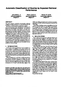
Automatic Classification of Seafloor Image Data by Geospatial Texture Descriptors Dissertation

zur Erlangung des Grades eines Doktors der Ingenieurwissenschaften - Dr.-Ing. -

vorgelegt im Fachbereich 3 (Mathematik und Informatik) der Universität Bremen im November 2014

Gutachter:

Prof. Dr. Otthein Herzog Universität Bremen Prof. Dr. Michael Schl¨ uter Alfred-Wegener-Institut f¨ ur Polar- und Meeresforschung

Disputation:

19. Dezember 2014

Acknowledgements I would like to cordially thank all people who supported me in the creation of this thesis, first and foremost my principal supervisor Prof. Dr. Otthein Herzog as well as my second supervisor Prof. Dr. Michael Schl¨ uter. Without your professional and personal advice, this work would not have been possible. I greatly appreciate the cooperation with my colleagues from the Artificial Intelligence Group at the Center for Computing Technologies (TZI) as well as the graduate school Advances in Digital Media at Bremen University. I am very grateful to all of you for all the fruitful discussions and suggestions. I am very thankful to Dr. Kerstin Jerosch who supported this work as a domain expert in the preparation of ground-truth data as well as by providing the reference data from Jerosch [2006]. Working with you was a pleasure and I am looking forward to future cooperation. I would further like to thank the Alfred Wegener Institute for Polar and Marine Research (AWI) and the French Research Institute for Exploration of the Sea (IFREMER) for the permission to use the image data produced in the framework of the AWI-IFREMER bilateral collaboration. To my friends and family I would like to express my sincere gratitude for your patience and encouragement throughout the preparation of this work, above all my wife Martina and my parents Irmgard and Heinz L¨ udtke.

iii

iv

Abstract A novel approach for automatic context-sensitive classification of spatially distributed image data is introduced. The proposed method targets applications of seafloor habitat mapping but is generally not limited to this domain or use case. Spatial context information is incorporated in a two-stage classification process, where in the second step a new descriptor for patterns of feature class occurrence according to a generically defined classification scheme is applied. The method is based on supervised machine learning, where numerous state-of-the-art approaches are applicable. The descriptor computation originates from texture analysis in digital image processing. Patterns of feature class occurrence are perceived as a texture-like phenomenon and the descriptors are therefore denoted by Geospatial Texture Descriptors. The proposed method was extensively validated based on a set of more than 4000 georeferenced video mosaics acquired at the H˚ akon Mosby Mud Volcano north-west of Norway recorded during cruise ARK XIX3b of the German research vessel Polarstern. The underlying classification scheme was derived from a scheme developed for manual annotation of the same dataset applied in the course of Jerosch [2006]. Features of interest are related to methane discharge at mud volcanoes, which are considered a significant source of methane emission. In the experimental evaluation, based on the prepared training and test data, a major improvement of the classification precision compared to local classification as well as classification based on the raw data from the local spatial context was achieved by the application of the proposed method. The classification precision was particularly improved for rarely occurring classes. In a further comparison with annotated data available from Jerosch [2006] the regional setting of the investigation area obtained by the application of the proposed method was found almost equivalent to the results of an experienced scientist.

v

vi

Zusammenfassung Gegenstand der Arbeit ist ein neuartiger Ansatz zur Klassifikation r¨ aumlich verteilter Bilddaten. Das Verfahren wurde entwickelt im Hinblick auf Anwendungen zur Kartierung von Habitaten am Meeresboden. Es eignet sich jedoch generell zur Klassifikation r¨ aumlich verteilter Bilddaten in beliebigen Domänen. In einem zweistufigen Klassifikationsprozess wird, zusätzlich zu lokalen Bildmerkmalen, ein im Rahmen der Arbeit entwickelter Deskriptor zur Beschreibung r¨ aumlicher Anordnungen von Merkmalsklassen entsprechend eines gegebenen Klassifikationsschemas eingesetzt. Als Klassifikatoren werden etablierte u ¨berwachte Lernverfahren verwendet. Die Beschreibung r¨ amlicher Verteilungsmuster ist angelehnt an Verfahren aus dem Bereich der Texturanalyse in der Bildverarbeitung. Muster des Auftretens der Merkmalsklassen werden hierbei, ¨ ahnlich wie die r¨ aumliche Verteilung von Intensitätswerten in der Bildebene, als Textur aufgefasst. Der Deskriptor wird entsprechend mit Geospatial Texture Descriptor bezeichnet. Zur Evaluation wurde das Verfahren angewendet zur Klassifikation eines Datensatzes aus mehr als 4000 georeferenzierten Videomosaiken vom Meeresboden, die auf der Expedition ARK XIX3b des Forschungsschiffes Polarstern am H˚ akon Mosby Schlammvulkan nordwestlich der K¨ uste Norwegens aufgenommen wurden. Das zugrunde liegende Klassifikationsschema ist abgeleitet von einem Schema zur manuellen Annotation, das in Jerosch [2006] eingef¨ uhrt wurde. Ziel ist die Erkennung von Merkmalen, die mit der Emission von Methan an Schlammvulkanen in Zusammenhang stehen. Schlammvulkane werden als signifikante Quellen der Methanemission betrachtet. In den Experimenten zur Evaluation basierend auf den erstellten Trainings- und Testdatensätzen wurde, im Vergleich Klassifikation ausschließlich basierend auf lokalen Bildmerkmalen, sowie im Vergleich zu den rohen Merkmalen und auftretenden Merkmalsklassen aus der lokalen Nachbarschaft als Kontextinformation, eine deutliche Verbesserung der Klassifikation erreicht. Dabei wurde speziell die Erkennung selten auftretender Merkmalsklassen erheblich verbessert. In einem Vergleich mit den aus Jerosch [2006] verf¨ ugbaren Daten entsprachen die Ergebnisse der automatischen Klassifikation durch das vorgeschlagene Verfahren weitgehend den Annotationen eines erfahrenen Domänenexperten. Die sich ergebende r¨ aumliche Struktur der Untersuchungsregion war nahezu identisch.

vii

viii

Contents Abstract

v

List of Figures

xiii

List of Tables

xxiii

Listings

xxxi

1 Introduction

1

2 Related Work 2.1 Image-Based Texture Analysis and Description . . . . . . . . . . 2.2 Recent Extensions and Applications of Haralick’s Co-occurrencebased Approach . . . . . . . . . . . . . . . . . . . . . . . . . . . . 2.3 Analysis and Classification of Spatially Distributed Image Data in Remote Sensing . . . . . . . . . . . . . . . . . . . . . . . . . . 2.4 Benthic Habitat Mapping and Image Analysis in the Underwater Domain . . . . . . . . . . . . . . . . . . . . . . . . . . . . . . . . 2.5 Submarine Mud Volcanoes / H˚ akon Mosby Mud Volcano . . . . 2.6 Comparison of Selected Related Works . . . . . . . . . . . . . . .

5 6 9 11 14 18 19

3 Classification by Geospatial Texture Descriptors 23 3.1 General Approach . . . . . . . . . . . . . . . . . . . . . . . . . . 24 3.2 World-Based Grid Overlain on the Image Data . . . . . . . . . . 24 3.3 Classification Scheme . . . . . . . . . . . . . . . . . . . . . . . . . 26 3.4 Local Classification by Low-Level Features Extracted From the Raw Image Data . . . . . . . . . . . . . . . . . . . . . . . . . . . 28 3.5 Computation and Application of Geospatial Texture Descriptors 34 3.5.1 Class Label Distribution and Co-occurrence . . . . . . . . 35 3.5.2 Features Computed From the Class Label Distribution and Co-occurrence . . . . . . . . . . . . . . . . . . . . . . 38 3.5.3 Composition of Geospatial Texture Descriptors . . . . . . 42 3.5.4 Application of Geospatial Texture Descriptors . . . . . . . 43 3.6 Selection of Locally Dominant Class Labels . . . . . . . . . . . . 45 3.7 Summary and Discussion . . . . . . . . . . . . . . . . . . . . . . 45 ix

x

CONTENTS

4 GIDAS - Geospatial Image Database and Analysis System 4.1 The GIDAS Application . . . . . . . . . . . . . . . . . . . . . . . 4.1.1 Spatial Image Database . . . . . . . . . . . . . . . . . . . 4.1.2 Map and Image View Modes and Plug-In Interface . . . . 4.1.3 Image Analysis and Batch Processing . . . . . . . . . . . 4.1.4 Map Visualisations and Storage and Export of Map-Based Data . . . . . . . . . . . . . . . . . . . . . . . . . . . . . . 4.2 Implementation of the Proposed Approach . . . . . . . . . . . . . 4.2.1 Generic Definition of World-Based Grids in an XML format 4.2.2 Generic Definition of Classification Schemes in an XML format . . . . . . . . . . . . . . . . . . . . . . . . . . . . . 4.2.3 User Interface for the Preparation of Training and Test Data . . . . . . . . . . . . . . . . . . . . . . . . . . . . . . 4.2.4 Extration of Low-Level Image Features . . . . . . . . . . 4.2.5 Local Classification Based on Low-Level Image Features . 4.2.6 Extraction of Geospatial Texture Descriptors . . . . . . . 4.2.7 Classification by Geospatial Texture Descriptors . . . . . 4.2.8 Model Creation and Parameter Selection . . . . . . . . . . 4.2.9 Export of Classification Results . . . . . . . . . . . . . . . 4.3 Summary and Discussion . . . . . . . . . . . . . . . . . . . . . .

47 48 48 48 49 49 51 51 53 55 56 57 57 57 58 59 59

5 Automatic Classification of Seafloor Image Data from the H˚ akon Mosby Mud Volcano 61 5.1 Underlying Image Dataset . . . . . . . . . . . . . . . . . . . . . . 64 5.2 Classification Scheme . . . . . . . . . . . . . . . . . . . . . . . . . 65 5.3 Machine Learning Schemes and Parameter Selection . . . . . . . 67 5.4 Experimental Selection of Cell Size . . . . . . . . . . . . . . . . . 69 5.5 Preparation of Training and Test Data . . . . . . . . . . . . . . . 77 5.6 Experimental Results . . . . . . . . . . . . . . . . . . . . . . . . . 79 5.6.1 Results Obtained Using Different Descriptor Types and Varying Distance and Neighbourhood Size . . . . . . . . . 82 5.6.2 Map Visualisations of the Results Obtained . . . . . . . . 99 5.6.3 Result Improvement by Geospatial Texture Descriptors . 104 5.6.4 Comparison With Results Obtained by Majority Filtering 110 5.6.5 Comparison With Classification Based on the Raw Neighbourhood of Cells . . . . . . . . . . . . . . . . . . . . . . 112 5.7 Comparison With Further Visually Inspected Field Data . . . . . 126 5.8 Summary and Discussion . . . . . . . . . . . . . . . . . . . . . . 133 6 Conclusions and Future Work

135

Bibliography

139

Appendix A Dataset of Exemplary Images for the Feature Classes of the Classification Scheme 155

CONTENTS

xi

Appendix B Detailed Experimental Results of the Cell Size Selection for the H˚ akon Mosby Image Dataset 171 Appendix C Detailed Experimental Classification Results for the H˚ akon Mosby Image Dataset 179 C.1 Classification Results Obtained by the Application of Geospatial Texture Descriptors . . . . . . . . . . . . . . . . . . . . . . . . . 180 C.2 Classification Based on the Raw Neighbourhood of Cells . . . . . 217

xii

CONTENTS

List of Figures

3.1

Sample image (a) without and (b) with grid cells overlain. Different classes assigned according to the underlying classification scheme are indicated by different colours. This sample image is part of the dataset underlying the evaluation of the proposed approach presented in Chapter 5 : Automatic Classification of Seafloor Image Data from the H˚ akon Mosby Mud Volcano. . . .

27

Four directions of co-occurring adjacent pixels in the matrix computation for a pixel-distance of dG = 1. . . . . . . . . . . . . . .

30

3.3

Overview of the proposed two-stage classification procedure. . . .

44

4.1

The two main view modes of the GIDAS application. (a) GIDAS image view. The image view provides a plugin interface enabling modules to integrate overlays of analysis results or interaction interfaces, e.g. for image annotation. (b) Map view of the GIDAS application for spatial, map-based presentation of analysis results. . . . . . . . . . . . . . . . . . . . . . . . . . . . . . . . .

50

Annotation interface integrated as a plugin for the GIDAS image view. A set of world-based grid cells is labelled manually by a domain expert as training data for the machine learning classifiers based on a scheme generically defined as described in Section 4.2.1 : Generic Definition of World-Based Grids in an XML format where also overlay colours are specified for each class. Colours refer to a classification scheme applied to the classification of image data from mud volcanoes. Green: Smooth Mud ; blue: Structured Mud ; white: Beggiatoa; red: Pogonophora. . . .

56

3.2

4.2

xiii

xiv

LIST OF FIGURES 5.1

5.2

5.3

5.4

5.5

5.6

Regional setting at the H˚ akon Mosby Mud Volcano: The H˚ akon Mosby Mud Volcano is about 1.4 km in diameter in water depths of 1250 − 1266 m [Vogt et al., 1997]. It is a concentric morphologic structure with highly gas-saturated sediments. A flat central area of grey fluid-like mud with a high geothermal gradient [Kaul et al., 2006] is surrounded by a zone of bacterial mats. This centre is surrounded by elevated sediment features (relief-rich zone) densely populated by Pogonophora tube worms [Jerosch et al., 2007b]. Video transects underlying the evaluation of the proposed approach in this chapter are marked, where black segments indicate image data annotated in the course of Jerosch [2006] and white segments the remaining data available. (Taken from L¨ udtke et al. [2012]) . . . . . . . . . . . . . . . . . . . . . .

63

(a) Underwater ROV Victor6000. (b) Screenshot of the MATISSE software (images by IFREMER, France). . . . . . . . . .

64

Examples for different habitat categories at the H˚ akon Mosby Mud Volcano: (a) Beggiatoa patches 20 − 50%, (b) Beggiatoa mats > 50%, (c) Beggiatoa patches < 20% and Pogonophora 50 − 80%, (d) Pogonophora > 80%, (e) 100% Structured Mud and (f) 100% Smooth Mud with ripples. (Taken from L¨ udtke et al. [2012], images recorded by Victor6000 /IFREMER) . . . .

65

Changing areas of tube worms and bacterial mats within a 20 m video mosaicing stripe north-west of the centre of the H˚ akon Mosby Mud Volcano. Five single georeferenced video mosaics have been catenated by overlay applying a GIS. (Taken from L¨ udtke et al. [2012]) . . . . . . . . . . . . . . . . . . . . . . . . .

66

Different cell sizes overlain on a sample image: (a) 0.2 m × 0.2 m, (b) 0.4 m × 0.4 m, (c) 0.6 m × 0.6 m, (d) 0.8 m × 0.8 m and (e) 1.0 m × 1.0 m. Based on the procedure described in Section 5.4 a cell size of 0.6 m × 0.6 m as visualised in (c) was finally selected for the subsequent experiments. (Images recorded by Victor6000 /IFREMER) . . . . . . . . . . .

70

Experimental selection of the size of world-based cells: F-measures for each class obtained by the application of Support Vector Machines [Vapnik, 1995] to small sets of sample images annotated using different cell sizes. The best average F-measure was obtained applying a cell size of 0.6 m × 0.6 × m. . . . . . . . . . .

74

LIST OF FIGURES 5.7

xv

Experimental selection of the size of world-based cells: F-measures for each class obtained by the application of the k-Nearest Neighbour classifier [Aha et al., 1991] to small sets of sample images annotated using different cell sizes. The best average F-measure was obtained applying a cell size of 0.6 m × 0.6 × m. . . . . . .

75

Experimental selection of the size of world-based cells: F-measures for each class obtained by the application of the C4.5 Decision Tree classifier [Quinlan, 1993] on small sets of sample images annotated using different cell sizes. The best average F-measure was obtained applying a cell size of 0.6 m × 0.6 × m. . . . . . .

76

Two sample images from the manually annotated dataset with and without annotations marked. Coloured cells correspond to feature classes as follows: red → Pogonophora, white → Beggiatoa, green → Smooth Mud, and blue → Structured Mud. (a) and (b): Neighbouring regions of Pogonophora and Beggiatoa. (c) and (d): Neighbouring regions of Beggiatoa and Structured Mud, separated by a small band of Smooth Mud. (Images recorded by Victor6000 /IFREMER) . . . . . . . . . . .

78

5.10 Spatial distribution of the overall image dataset and the set annotated as training and test data. (Screen capture of map view of the GIDAS application developed in the course of this work, see Chapter 4 : GIDAS - Geospatial Image Database and Analysis System.) (a) Map of image data manually annotated as training and test set. (b) Map of complete image dataset. . . . . . . . .

80

5.11 Classification performance obtained by the application of Support Vector Machines [Vapnik, 1995] using Geospatial Texture C for varying parameter values of neighDescriptors of type DD bourhood size sC and distance dC (the source data of this diagram is included in Section C.1 : Classification Results Obtained by the Application of Geospatial Texture Descriptors of Appendix C : Detailed Experimental Classification Results for the H˚ akon Mosby Image Dataset in Table C.1). . . . . . . . . . . . . . . . .

86

5.12 Classification performance obtained by the application of Support Vector Machines [Vapnik, 1995] using Geospatial Texture Descriptors of type DFC for varying parameter values of neighbourhood size sC and distance dC (the source data of this diagram is included in Section C.1 : Classification Results Obtained by the Application of Geospatial Texture Descriptors of Appendix C : Detailed Experimental Classification Results for the H˚ akon Mosby Image Dataset in Table C.2). . . . . . . . . . . . . . . . .

87

5.8

5.9

xvi

LIST OF FIGURES 5.13 Classification performance obtained by the application of Support Vector Machines [Vapnik, 1995] using Geospatial Texture C Descriptors of type DDF for varying parameter values of neighbourhood size sC and distance dC (the source data of this diagram is included in Section C.1 : Classification Results Obtained by the Application of Geospatial Texture Descriptors of Appendix C : Detailed Experimental Classification Results for the H˚ akon Mosby Image Dataset in Table C.3). . . . . . . . . . . . . . . . .

88

5.14 Classification performance obtained by the application of the kNearest Neighbour classifier [Aha et al., 1991] using Geospatial C Texture Descriptors of type DD for varying parameter values of neighbourhood size sC and distance dC (the source data of this diagram is included in Section C.1 : Classification Results Obtained by the Application of Geospatial Texture Descriptors of Appendix C : Detailed Experimental Classification Results for the H˚ akon Mosby Image Dataset in Table C.4). . . . . . . . . .

91

5.15 Classification performance obtained by the application of the kNearest Neighbour classifier [Aha et al., 1991] using Geospatial Texture Descriptors of type DFC for varying parameter values of neighbourhood size sC and distance dC (the source data of this diagram is included in Section C.1 : Classification Results Obtained by the Application of Geospatial Texture Descriptors of Appendix C : Detailed Experimental Classification Results for the H˚ akon Mosby Image Dataset in Table C.5). . . . . . . . . .

92

5.16 Classification performance obtained by the application of the kNearest Neighbour classifier [Aha et al., 1991] using Geospatial C for varying parameter values Texture Descriptors of type DDF of neighbourhood size sC and distance dC (the source data of this diagram is included in Section C.1 : Classification Results Obtained by the Application of Geospatial Texture Descriptors of Appendix C : Detailed Experimental Classification Results for the H˚ akon Mosby Image Dataset in Table C.6). . . . . . . . . . . . .

93

5.17 Classification performance obtained by the application of the C4.5 Decision Tree classifier [Quinlan, 1993] using Geospatial C Texture Descriptors of type DD for varying parameter values of neighbourhood size sC and distance dC (the source data of this diagram is included in Section C.1 : Classification Results Obtained by the Application of Geospatial Texture Descriptors of Appendix C : Detailed Experimental Classification Results for the H˚ akon Mosby Image Dataset in Table C.7). . . . . . . . . . . . .

96

LIST OF FIGURES

xvii

5.18 Classification performance obtained by the application of the C4.5 Decision Tree classifier [Quinlan, 1993] using Geospatial Texture Descriptors of type DFC for varying parameter values of neighbourhood size sC and distance dC (the source data of this diagram is included in Section C.1 : Classification Results Obtained by the Application of Geospatial Texture Descriptors of Appendix C : Detailed Experimental Classification Results for the H˚ akon Mosby Image Dataset in Table C.8). . . . . . . . . . . . .

97

5.19 Classification performance obtained by the application of the C4.5 Decision Tree classifier [Quinlan, 1993] using Geospatial C for varying parameter values Texture Descriptors of type DDF of neighbourhood size sC and distance dC (the source data of this diagram is included in Section C.1 : Classification Results Obtained by the Application of Geospatial Texture Descriptors of Appendix C : Detailed Experimental Classification Results for the H˚ akon Mosby Image Dataset in Table C.9). . . . . . . . . . . . .

98

5.20 Map visualisation of the classification results obtained by the application of Support Vector Machines [Vapnik, 1995] with Geospatial Texture Descriptors to the complete image dataset (best run for this learning scheme as well as best overall result). The correct classification rate was 90.73%. Results have been overlain on a visualisation of bathymetry data recorded at the H˚ akon Mosby Mud Volcano. . . . . . . . . . . . . . . . . . . . . . . . . . . . . 101

5.21 Map visualisation of the classification results obtained by the application of the k-Nearest Neighbour classifier [Aha et al., 1991] with Geospatial Texture Descriptors to the complete image data set (best run for this learning scheme). The correct classification rate was 85.55%. Results have been overlain on a visualisation of bathymetry data recorded at the H˚ akon Mosby Mud Volcano. . 102

5.22 Map visualisation of the classification results obtained by the application of the C4.5 Decision Tree classifier [Quinlan, 1993] with Geospatial Texture Descriptors to the complete image data set (best run for this learning scheme). The correct classification rate was 87.57%. Results have been overlain on a visualisation of bathymetry data recorded at the H˚ akon Mosby Mud Volcano. . 103

xviii

LIST OF FIGURES

5.23 Comparison of the results obtained by majority filtering of the local classification results based on a neighbourhood of varying size sC = 1, 2, .., 50 with the best results obtained in the two classification steps of the proposed approach - local classification and contextual classification using Geospatial Texture Descriptors. The results are visualised for the different learning schemes applied in the evaluation (SVM : Support Vector Machines, KNN : k-Nearest Neighbour classifier, C4.5 : C4.5 Decision Tree classifier; results of majority filtering for KNN and C4.5 are very close and overlap in the visualisation). In no case an increased classification precision was achieved by majority filtering. . . . . 111 5.24 Comparison of the results obtained by the application of Support Vector Machines [Vapnik, 1995] to the raw low-level image features in the local neighbourhood of varying size sC with the best results obtained in the two classification steps of the proposed approach - local classification and contextual classification using Geospatial Texture Descriptors (GTD). (The source data of this diagram is included in Section C.2 : Classification Based on the Raw Neighbourhood of Cells of Appendix C : Detailed Experimental Classification Results for the H˚ akon Mosby Image Dataset in Table C.10.) . . . . . . . . . . . . . . . . . . . . . . . . . . . . . 116 5.25 Comparison of the results obtained by the application of the kNearest Neighbour classifier [Aha et al., 1991] to the raw low-level image features in the local neighbourhood of varying size sC with the best results obtained in the two classification steps of the proposed approach - local classification and contextual classification using Geospatial Texture Descriptors (GTD). Missing runs did not terminate within a week. (The source data of this diagram is included in Section C.2 : Classification Based on the Raw Neighbourhood of Cells of Appendix C : Detailed Experimental Classification Results for the H˚ akon Mosby Image Dataset in Table C.10.) . . . . . . . . . . . . . . . . . . . . . . . . . . . . . . . . . 117 5.26 Comparison of the results obtained by the application of the C4.5 Decision Tree classifier [Quinlan, 1993] to the raw low-level image features in the local neighbourhood of varying size sC with the best results obtained in the two classification steps of the proposed approach - local classification and contextual classification using Geospatial Texture Descriptors (GTD). (The source data of this diagram is included in Section C.2 : Classification Based on the Raw Neighbourhood of Cells of Appendix C : Detailed Experimental Classification Results for the H˚ akon Mosby Image Dataset in Table C.10.) . . . . . . . . . . . . . . . . . . . . . . . . . . . . 118

LIST OF FIGURES

xix

5.27 Comparison of the results obtained by the application of Support Vector Machines [Vapnik, 1995] to a subset of preselected low-level image features in the local neighbourhood of varying size sC with the best results obtained in the two classification steps of the proposed approach - local classification and contextual classification using Geospatial Texture Descriptors (GTD). (The source data of this diagram is included in Section C.2 : Classification Based on the Raw Neighbourhood of Cells of Appendix C : Detailed Experimental Classification Results for the H˚ akon Mosby Image Dataset in Table C.11.) . . . . . . . . . . . . . . . 119 5.28 Comparison of the results obtained by the application of the kNearest Neighbour classifier [Aha et al., 1991] to a subset of preselected low-level image features in the local neighbourhood of varying size sC with the best results obtained in the two classification steps of the proposed approach - local classification and contextual classification using Geospatial Texture Descriptors (GTD). Missing runs did not terminate within a week. (The source data of this diagram is included in Section C.2 : Classification Based on the Raw Neighbourhood of Cells of Appendix C : Detailed Experimental Classification Results for the H˚ akon Mosby Image Dataset in Table C.11.) . . . . . . . . . . . . . . . 120 5.29 Comparison of the results obtained by the application of the C4.5 Decision Tree classifier [Quinlan, 1993] to a subset of preselected low-level image features in the local neighbourhood of varying size sC with the best results obtained in the two classification steps of the proposed approach - local classification and contextual classification using Geospatial Texture Descriptors (GTD). Missing runs did not terminate within a week. (The source data of this diagram is included in Section C.2 : Classification Based on the Raw Neighbourhood of Cells of Appendix C : Detailed Experimental Classification Results for the H˚ akon Mosby Image Dataset in Table C.11.) . . . . . . . . . . . . . . . . . . . . . . . . . . . . . 121 5.30 Comparison of the results obtained by the application of Support Vector Machines [Vapnik, 1995] to the raw class labels in the local neighbourhood of varying size sC with the best results obtained in the two classification steps of the proposed approach - local classification and contextual classification using Geospatial Texture Descriptors (GTD). (The source data of this diagram is included in Section C.2 : Classification Based on the Raw Neighbourhood of Cells of Appendix C : Detailed Experimental Classification Results for the H˚ akon Mosby Image Dataset in Table C.11.) . . . . . . . . . . . . . . . . . . . . . . . . . . . . . . . . . 123

xx

LIST OF FIGURES 5.31 Comparison of the results obtained by the application of the kNearest Neighbour classifier [Aha et al., 1991] to the raw class labels in the local neighbourhood of varying size sC with the best results obtained in the two classification steps of the proposed approach - local classification and contextual classification using Geospatial Texture Descriptors (GTD). (The source data of this diagram is included in Section C.2 : Classification Based on the Raw Neighbourhood of Cells of Appendix C : Detailed Experimental Classification Results for the H˚ akon Mosby Image Dataset in Table C.11.) . . . . . . . . . . . . . . . . . . . . . . . . . . . . 124

5.32 Comparison of the results obtained by the application of the C4.5 Decision Tree classifier [Quinlan, 1993] to the raw class labels in the local neighbourhood of varying size sC with the best results obtained in the two classification steps of the proposed approach - local classification and contextual classification using Geospatial Texture Descriptors (GTD). (The source data of this diagram is included in Section C.2 : Classification Based on the Raw Neighbourhood of Cells of Appendix C : Detailed Experimental Classification Results for the H˚ akon Mosby Image Dataset in Table C.11.) . . . . . . . . . . . . . . . . . . . . . . . . . . . . . . . . . 125

5.33 Deviation of the feature coverage automatically detected by the application of the proposed approach using Support Vector Machines [Vapnik, 1995] and manually annotated for the Pogonophora class visualised as a colour ramp. Yellow to green: overestimation in the automatic detection of feature coverage, yellow to red: underestimation in the automatic detection of feature coverage. Reference polygons have been annotated by a domain expert in the course of Jerosch [2006]. Results have been overlain on a visualisation of bathymetry data recorded at the H˚ akon Mosby Mud Volcano. . . . . . . . . . . . . . . . . . . . . . . . . . . . . 129

5.34 Deviation of the feature coverage automatically detected by the application of the proposed approach using Support Vector Machines [Vapnik, 1995] and manually annotated for the Beggiatoa class visualised as a colour ramp. Yellow to green: overestimation in the automatic detection of feature coverage, yellow to red: underestimation in the automatic detection of feature coverage. Reference polygons have been annotated by a domain expert in the course of Jerosch [2006]. Results have been overlain on a visualisation of bathymetry data recorded at the H˚ akon Mosby Mud Volcano. . . . . . . . . . . . . . . . . . . . . . . . . . . . . 130

LIST OF FIGURES

xxi

5.35 Deviation of the feature coverage automatically detected by the application of the proposed approach using Support Vector Machines [Vapnik, 1995] and manually annotated for the Smooth Mud class visualised as a colour ramp. Yellow to green: overestimation in the automatic detection of feature coverage, yellow to red: underestimation in the automatic detection of feature coverage. Reference polygons have been annotated by a domain expert in the course of Jerosch [2006]. Results have been overlain on a visualisation of bathymetry data recorded at the H˚ akon Mosby Mud Volcano. . . . . . . . . . . . . . . . . . . . . . . . . . . . . 131 5.36 Deviation of the feature coverage automatically detected by the application of the proposed approach using Support Vector Machines [Vapnik, 1995] for classification and manually annotated for the Structured Mud class visualised as a colour ramp. Yellow to green: overestimation in the automatic detection of feature coverage, yellow to red: underestimation in the automatic detection of feature coverage. Reference polygons have been annotated by a domain expert in the course of Jerosch [2006]. Results have been overlain on a visualisation of bathymetry data recorded at the H˚ akon Mosby Mud Volcano. . . . . . . . . . . . . . . . . . . 132

xxii

LIST OF FIGURES

List of Tables

2.1

3.1

3.2

3.3

Schematic comparison of selected works closely related to the method proposed in this work in different aspects. Part of the works refers to spatial contextual image classification in general applications of remote sensing with a distinct representation of microtexture and macrotexture similar to the proposed method. Other works present methods applied to sediment classification in seafloor habitat mapping not necesarily employing contextual information in the classification process. . . . . . . . . . . . . .

21

Set of low-level image features proposed for application in the first classification step. The low-level image features are computed from the local grey level distributions based on the frequency of individual grey levels and grey level co-occurrence inside the single grid cells ci,j ∈ G (see Section 3.2 : World-Based Grid Overlain on the Image Data). . . . . . . . . . . . . . . . . . . .

32

Feature set comprising the local frequencies of occurrence and co-occurrence of class labels in the neighbourhood NsC (gi,j ) of a grid cell gi,j ∈ G applied in the second classification step of the C proposed approach. As of the symmetry of Pi,j the total amount 2 C < N . of unique CLCM-based feature values is only NPi,j . . . C

37

Set of features extracted from the first and second order statistics describing the class label occurrence and co-occurrence in the neighbourhood NsC (gi,j ) of a grid cell ci,j ∈ G applied in the second classification step of the proposed approach. . . . . . . .

41

xxiii

xxiv 5.1

5.2

5.3

5.4

5.5

5.6

LIST OF TABLES Original annotation scheme for manual annotation of sediment image data from mud volcanoes as introduced by Jerosch [2006]. Annotation is based on polygons much larger than the cells in the approach proposed in this work. Therefore, coverage classes as presented are assigned in the manual annotation for each polygon and feature class. The classification scheme applied in this work is based on the feature classes defined here. . . . . . . . . . . . .

67

Classification scheme underlying the cell-based automatic classification of seafloor image data from mud volcanoes in the evaluation of the proposed approach. The scheme is derived from the annotation scheme introduced by Jerosch [2006] for manual annotation as displayed in Table 5.1. . . . . . . . . . . . . . . .

67

Machine learning schemes applied in the course of the evaluation of the proposed approach. The approach for context description and context-sensitive classification proposed in this work is generally independent of the specific machine learning scheme applied. Three well-established machine learning schemes of different types have been used. In the selection of the scheme parameters, the configurations as presented here have been applied. . . . . . . . . . . . . . . . . . . . . . . . . . . . . . . . . . . . . .

68

Average size of cells overlain on the image data in pixels for the different cell sizes tested in the experimental selection. The image-based size of grid cells slightly varies due to varying height over ground of the remotely operated vehicle (ROV). Finally selected was a cell size of 0.6 m × 0.6 m, so the average size of cells overlain on the image data was 65 × 65 px in the subsequent experiments. . . . . . . . . . . . . . . . . . . . . . . . . . . . . . .

71

Comparison of the confusion matrices for the best runs for each cell size expressed as a percentage. The best results were obtained by the application of Support Vector Machines [Vapnik, 1995] in all cases. (More detailed presentations including total frequencies and the results for all learning schemes are available in the Appendix B : Detailed Experimental Results of the Cell Size Selection for the H˚ akon Mosby Image Dataset in the Tables B.1, B.2, and B.3.) . . . . . . . . . . . . . . . . . . . . . . . . .

72

Class distribution resulting from manual labelling of sample image data by a human domain expert. 14 366 cells in 275 sample images selected by the domain expert have been labelled based on the classification scheme presented in Table 5.2. . . . . . . .

77

LIST OF TABLES 5.7

xxv

Comparison of the classification performance obtained for the training and test data by local classification and classification with the proposed Geospatial Texture Descriptors (GTD). An improvement in the correct classification rate of up to ≈ 6.89% was achieved by the application of GTD. . . . . . . . . . . . . .

81

Classification performance obtained by the application of Support Vector Machines [Vapnik, 1995] : comparison of local classification and classification with Geospatial Texture Descriptors (GTD) using the different descriptor types. An improvement in the correct classification rate of up to 3.40% was achieved by the application of GTD. . . . . . . . . . . . . . . . . . . . . . . . . .

84

Classification performance obtained by the application of the kNearest Neighbour classifier [Aha et al., 1991] : comparison of local classification and classification with Geospatial Texture Descriptors (GTD) using the different descriptor types. An improvement in the overall classification rate of up to 4.69% was achieved by the application of GTD. . . . . . . . . . . . . . . . .

89

5.10 Classification performance obtained by the application of the C4.5 decision tree classifier [Quinlan, 1993] : comparison of local classification and classification with Geospatial Texture Descriptors (GTD) using the different descriptor types. An improvement in the correct classification rate of up to 6.89% was achieved by the application of GTD. . . . . . . . . . . . . . . . . . . . . . . .

94

5.11 Neighbourhood sizes obtained in the selection of locally dominant class labels as proposed in Section 3.6 : Selection of Locally Dominant Class Labels for the visualisation of the overall best classification result displayed in Figure 5.20 (results obtained by the application of Support Vector Machines [Vapnik, 1995] using C a Geospatial Texture Descriptor of type DD ). . . . . . . . . . .

99

5.8

5.9

5.12 Improvement of the classification precision in terms of relative frequencies of specific inter-class confusions for pairs of classes of the underlying classification scheme based on comparison of the best runs in the local classification stage and classification using the proposed Geospatial Texture Descriptors. The results for the different machine learning schemes are presented in separate table sections. On the main diagonals: improvement of the class-specific correct classification rates. . . . . . . . . . . . . . . 105

xxvi

LIST OF TABLES

5.13 Comparison of the confusion matrices for the best performing models in local classification based on low-level image features and classification using the proposed Geospatial Texture Descriptors (GTD) obtained by the application of Support Vector Machines [Vapnik, 1995]. . . . . . . . . . . . . . . . . . . . . . . . . 107 5.14 Comparison of the confusion matrices for the best performing models in local classification based on low-level image features and classification using the proposed Geospatial Texture Descriptors (GTD) obtained by the application of the k-Nearest Neighbour classifier [Aha et al., 1991]. . . . . . . . . . . . . . . . . . . 108 5.15 Comparison of the confusion matrices for the best performing models in local classification based on low-level image features and classification using the proposed Geospatial Texture Descriptors (GTD) obtained by the application of the C4.5 Decision Tree classifier [Quinlan, 1993]. . . . . . . . . . . . . . . . . . . . . . . 109 5.16 Correct classification rates obtained in the best runs applying the different machine learning schemes as introduced in Section 5.3 : Machine Learning Schemes and Parameter Selection based on the local set of preselected low-level image features. . . . . . 113 5.17 Correct classification rates obtained in the best runs applying the different machine learning schemes as introduced in Section 5.3 : Machine Learning Schemes and Parameter Selection based on raw low-level image features in the local neighbourhood of cells. . . . . . . . . . . . . . . . . . . . . . . . . . . . . . . . . . 114 5.18 Correct classification rates obtained in the best runs applying the different machine learning schemes to the raw class labels obtained from the first local classification step in the local neighbourhood of cells replacing the proposed Geospatial Texture Descriptors. . . . . . . . . . . . . . . . . . . . . . . . . . . . . . . . 122 5.19 Average measurable absolute error, underestimation, and overestimation for the results obtained by the application of the proposed approach using the different machine learning schemes applied in this evaluation compared to the polygon-based image annotations available from Jerosch [2006]: measurable distances in the estimated feature coverage for the different feature classes (see Section 5.2 : Classification Scheme). . . . . . . . . . . . . . 128

LIST OF TABLES

xxvii

A.1 Image dataset annotated for the experimental selection of the size of world-based grid cells as described in Section 5.4 : Experimental Selection of Cell Size. The dataset contains selected exemplary images for each class of the underlying classification scheme (see Table 5.2 in Chapter 5 : Automatic Classification of Seafloor Image Data from the H˚ akon Mosby Mud Volcano). (Images recorded by Victor6000 /IFREMER) . . . . . . . . . . . 156

B.1 Comparison of the confusion matrices obtained by the application of Support Vector Machines [Vapnik, 1995] for the different cell sizes used in the experimental selection. A visualisation of the F-measures obtained for each class and overall for the different cell sizes is available in Figure 5.6 in Section 5.4 : Experimental Selection of Cell Size. . . . . . . . . . . . . . . . . . . . . . . . . 172 B.2 Comparison of confusion matrices obtained by the application of the k-Nearest Neighbour classifier [Aha et al., 1991] for the different sizes tested in the experimental selection. A visualisation of the F-measures obtained for each class and overall compared for the different cell sizes is available in Figure 5.7 in Section 5.4 : Experimental Selection of Cell Size. . . . . . . . . . . . . . 174 B.3 Comparison of confusion matrices obtained by the application of the C4.5 Decision Tree classifier [Quinlan, 1993] for the different sizes tested in the experimental selection. A visualisation of the F-measures obtained for each class and overall compared for the different cell sizes is available in Figure 5.8 in Section 5.4 : Experimental Selection of Cell Size. . . . . . . . . . . . . . . . . . 176 C descriptor with C.1 Detailed classification results obtained for the DD varying distance and neighbourhood size using Support Vector Machines [Vapnik, 1995] as classifiers (see Figure 5.11 in Section 5.6.1 : Results Obtained Using Different Descriptor Types and Varying Distance and Neighbourhood Size of Chapter 5 : Automatic Classification of Seafloor Image Data from the H˚ akon Mosby Mud Volcano for a visualisation of this data). . . . . . . 181

C.2 Detailed classification results obtained for the DFC descriptor with varying distance and neighbourhood size using Support Vector Machines [Vapnik, 1995] as classifiers (see Figure 5.12 in Section 5.6.1 : Results Obtained Using Different Descriptor Types and Varying Distance and Neighbourhood Size of Chapter 5 : Automatic Classification of Seafloor Image Data from the H˚ akon Mosby Mud Volcano for a visualisation of this data). . . . . . . 185

xxviii

LIST OF TABLES

C C.3 Detailed classification results obtained for the DDF descriptor with varying distance and neighbourhood size using Support Vector Machines [Vapnik, 1995] as classifiers (see Figure 5.13 in Section 5.6.1 : Results Obtained Using Different Descriptor Types and Varying Distance and Neighbourhood Size of Chapter 5 : Automatic Classification of Seafloor Image Data from the H˚ akon Mosby Mud Volcano for a visualisation of this data). . . . . . . 189 C C.4 Detailed classification results obtained for the DD descriptor with varying distance and neighbourhood size using the k-Nearest Neighbour classifier [Aha et al., 1991] (see Figure 5.14 in Section 5.6.1 : Results Obtained Using Different Descriptor Types and Varying Distance and Neighbourhood Size of Chapter 5 : Automatic Classification of Seafloor Image Data from the H˚ akon Mosby Mud Volcano for a visualisation of this data). . . . . . . . . . . . . . . . . . . 193

C.5 Detailed classification results obtained for the DFC descriptor with varying distance and neighbourhood size using the k-Nearest Neighbour classifier [Aha et al., 1991] (see Figure 5.15 in Section 5.6.1 : Results Obtained Using Different Descriptor Types and Varying Distance and Neighbourhood Size of Chapter 5 : Automatic Classification of Seafloor Image Data from the H˚ akon Mosby Mud Volcano for a visualisation of this data). . . . . . . . . . . . . . . . . . . 197 C C.6 Detailed classification results obtained for the DDF descriptor with varying distance and neighbourhood size using the k-Nearest Neighbour classifier [Aha et al., 1991] (see Figure 5.16 in Section 5.6.1 : Results Obtained Using Different Descriptor Types and Varying Distance and Neighbourhood Size of Chapter 5 : Automatic Classification of Seafloor Image Data from the H˚ akon Mosby Mud Volcano for a visualisation of this data). . . . . . . 201 C descriptor with C.7 Detailed classification results obtained for the DD varying distance and neighbourhood size using the C4.5 Decision Tree classifier [Quinlan, 1993] (see Figure 5.17 in Section 5.6.1 : Results Obtained Using Different Descriptor Types and Varying Distance and Neighbourhood Size of Chapter 5 : Automatic Classification of Seafloor Image Data from the H˚ akon Mosby Mud Volcano for a visualisation of this data). . . . . . . 205

C.8 Detailed classification results obtained for the DFC descriptor with varying distance and neighbourhood size using the C4.5 Decision Tree classifier [Quinlan, 1993] (see Figure 5.18 in Section 5.6.1 : Results Obtained Using Different Descriptor Types and Varying Distance and Neighbourhood Size of Chapter 5 : Automatic Classification of Seafloor Image Data from the H˚ akon Mosby Mud Volcano for a visualisation of this data). . . . . . . 209

LIST OF TABLES

xxix

C C.9 Detailed classification results obtained for the DDF descriptor with varying distance and neighbourhood size using the C4.5 Decision Tree classifier [Quinlan, 1993] (see Figure 5.19 in Section 5.6.1 : Results Obtained Using Different Descriptor Types and Varying Distance and Neighbourhood Size of Chapter 5 : Automatic Classification of Seafloor Image Data from the H˚ akon Mosby Mud Volcano for a visualisation of this data). . . . . . . 213

C.10 Classification results obtained based on raw low-level image features and selected raw low-level image features in the local neighbourhood of cells for varying neighbourhood size (see Figure 5.24 for Support Vector Machines [Vapnik, 1995], Figure 5.25 for the k-Nearest Neighbour classifier, and Figure 5.26 for the C4.5 Decision Tree classifier in Section 5.6.5 : Comparison With Classification Based on the Raw Neighbourhood of Cells of Chapter 5 : Automatic Classification of Seafloor Image Data from the H˚ akon Mosby Mud Volcano for a visualisation of this data). . . . . . . 218 C.11 Classification results obtained based on preselected low-level features and raw labels in the local neighbourhood of cells for varying neighbourhood size (see Figures 5.27 and 5.30 for Support Vector Machines [Vapnik, 1995], Figures 5.28 and 5.31 for the k-Nearest Neighbour classifier and Figures 5.29 and 5.32 for the C4.5 Decision Tree classifier in Section 5.6.5 : Comparison With Classification Based on the Raw Neighbourhood of Cells of Chapter 5 : Automatic Classification of Seafloor Image Data from the H˚ akon Mosby Mud Volcano for a visualisation of this data). . . 220

xxx

LIST OF TABLES

Listings 4.1

XML schema for the definition of world-based grids.

. . . . . .

51

4.2

Definition of a world-based grid in XML. . . . . . . . . . . . . .

53

4.3

XML schema for the definition of classification schemes.

. . . .

53

4.4

Definition of a classification scheme in XML . . . . . . . . . . .

54

xxxi

xxxii

LISTINGS

Chapter 1

Introduction With the increasing application of underwater vehicles equipped with modern, high-resolution camera hardware, growing volumes of multimedia data are being acquired and the analysis of digital images data has become an important task within the marine sciences. Compared to the enormous amounts of valuable image and video data acquired in modern applications, often only small portions of the data and still mostly only predefined sequences are analysed. The analysis is typically performed manually which is a time-consuming and error-prone task. To benefit from the increasing volumes of high-resolution multimedia data, effective methods for a precise content-based analysis are required. Therefore, computer-aided or fully automatic analysis of multimedia data supported by automatic image processing will be highly important for a complete evaluation of the available and future datasets. Image-based classification in geographic and geoscientific applications has been extensively studied in the context of space-based or airborne applications of remote sensing [Schowengerdt, 2006], recently combined with automatic processing of the acquired image data. Automatic land use or land cover classification are popular applications [e.g. Hoberg and Rottensteiner, 2010, Gamba and Dell’Acqua, 2003]. In these applications, structures of interest mostly occur at a pixel or even sub-pixel scale and classification is typically pixel-based [Kobler et al., 2006]. For the classification, data items are described by feature vectors where textural features based on a statistical analysis of grey-tone spatial dependence (i.e. co-occurrence, Haralick et al. [1973], Haralick [1979]) in the image pane are very popular for a wide range of structures of interest [e.g. Puetz and Olsen, 2006, Kandaswamy et al., 2005, Maheshwary and Srivastava, 2009, Soh and Tsatsoulis, 1999] and the most widely used texture-based approach [Kandaswamy et al., 2005, Bekkari et al., 2012]. In a pixel-based classification 1

2

CHAPTER 1. INTRODUCTION

features of this type describe the spatial context or local spatial dependence of data items rather than single data items. This is particularly appropriate for geographic applications according to Tobler’s first law of geography [Tobler, 1970]: “Everything is related to everything else, but near things are more related than distant things.” Approaches taking into account the local spatial environment - also denoted by spatial contextual classification - generally lead to better classification results. An emerging application field in marine sciences is the mapping of benthic habitats by means of digital image data acquired by underwater platforms. In image-based seafloor habitat mapping [e.g. Vincent et al., 2003, Jerosch et al., 2006, 2011] modern systems are using high-resolution video information acquired by underwater platforms operating close to the seafloor. In contrast to space-based or airborne observations, investigation areas are often only sparsely covered by image data and the positioning is typically inexact. Structures of interest occur at different, mostly larger scales. While textural features like the above are still well-suited for the recognition of relevant structures [e.g. L¨ udtke et al., 2012], in this case the structures of interest themselves are described by the textural features rather than their spatial context. In this work, an approach for modeling the local spatial dependence of structures represented by classes of an underlying, generically defined classification scheme is proposed. A new type of descriptors for patterns of spatial co-occurrence of structures is introduced for the incorporation of contextual information in the classification process. The method has been designed targeting applications in seafloor habitat mapping for an automatic classification of spatially distributed, high-resolution image data with georeferencing available but is generally not limited to this application or domain. It translates statistical approaches for image-based texture description to the description of spatial patterns of feature class occurrence and co-occurrence according to a domainspecific classification scheme. Occurrence of local spatial patterns of structures of interest is perceived as a texture-like phenomenon denoted by the Geospatial Texture in this work. Numerical features extracted from these patterns form socalled Geospatial Texture Descriptors. The proposed approach has been worked out with specific regard to applications in the underwater domain in various aspects. This includes robustness with respect to the sparse data coverage of investigation areas as is typically the case in underwater imaging applications as well as sparse and unstable lighting resulting from energy limitations of underwater vehicles and inexact georeferencing due to positioning errors. The approach is therefore particularly well-suited for the proposed application of image-based seafloor habitat mapping as shown in the experimental evaluation part of this work. The proposed approach generally comprises two subsequent classification steps performed independently of each other. Based on a set of low-level image

3 features an initial classification of data items in a first, local classification step is performed. Single classification units are regular grid cells overlain on the image data. In the case of image-based seafloor habitat mapping, features based on grey-level co-occurrence are proposed and have been proven to work well for a broad range of structures of interest [e.g. L¨ udtke et al., 2012, Enomoto et al., 2011] while in general the method is generic also with regard to the set of image-based features employed. For specific domains other feature sets may help to improve the classification accuracy by reflecting domain specific properties. Based on this initial context-independent classification of data items the proposed descriptors for patterns of neighbouring structures, i.e. feature classes of the underlying classification scheme, are computed. These descriptors for the local spatial context of data items are then applied in a second contextual (re-)classification step. Classification in both steps is based on vectors of numerical features following the widely applied supervised learning paradigm where a large number of well-known, mature machine learning schemes such as Support Vector Machines [Vapnik, 1995] or decision trees [Quinlan, 1993] are applicable. The use of different techniques is explored in the course of this work. Models are trained for the supervised learning schemes based on sets of data labelled by domain experts, where the same dataset is employed for the training of classifiers in both classification steps. Therefore no additional human effort is introduced here. Given a pair of trained models for the two steps, large datasets can be classified fully automatically. Classification results benefit from the incorporation of contextual information in the classification process on the second level. In the experimental validation of this work this is demonstrated for the use case of image-based classification of benthic habitats where the underlying dataset was acquired at the H˚ akon Mosby Mud Volcano. The image data were recorded during cruise ARK XIX3b [Klages et al., 2004] of the German research vessel Polarstern in 2003 by the underwater remotely operated vehicle (ROV) Victor6000. Features of interest are related to methane discharge at mud volcanoes [e.g. Sauter et al., 2006, Niemann et al., 2006]. The classification scheme employed originates from a scheme introduced for manual annotation of seafloor image data from mud volcanoes in Jerosch [2006].

4

CHAPTER 1. INTRODUCTION

Chapter 2

Related Work The method proposed in this work for the automatic classification of spatially distributed, georeferenced image data translates statistical approaches for image-based texture description to the description of spatial patterns of feature class occurrence according to a generically defined, domain-specific classification scheme. Patterns of feature class occurrence are perceived as a texture-like phenomenon, therefore denoted by the Geospatial Texture. Features extracted from that are combined into so-called Geospatial Texture Descriptors and applied within a two-stage classification process using standard supervised machine learning techniques such as Support Vector Machines or decision tree classifiers. In the following sections, related work from different relevant fields with regard to the method is presented. Section 2.1 : Image-Based Texture Analysis and Description introduces different approaches for image-based texture analysis and description. Features of this kind are applied in the first classification step of the proposed two-stage classification process as well as translated to the description of patterns of feature class occurrence in the second classification step. In Section 2.2 : Recent Extensions and Applications of Haralick’s Co-occurrence-based Approach other recent extensions of the underlying method originally introduced in Haralick et al. [1973] are presented. Section 2.3 : Analysis and Classification of Spatially Distributed Image Data in Remote Sensing then describes recent approaches applied to the automatic analysis and classification of spatially distributed image data. The following Section 2.4 : Benthic Habitat Mapping and Image Analysis in the Underwater Domain focuses on approaches applied to benthic habitat mapping in the underwater domain, which is the main targeted application field of the proposed method. Here, related work includes the manual analysis of seafloor image data as well as approaches involving automatic image analysis and classification for benthic habitat mapping. Finally, Section 5

6

CHAPTER 2. RELATED WORK

2.5 : Submarine Mud Volcanoes / H˚ akon Mosby Mud Volcano presents related work referring to submarine mud volcanoes and specifically the H˚ akon Mosby Mud Volcano, where the proposed method has been successfully applied to sediment classification and the detection of seafloor features related to the scientific investigation of methane discharge at mud volcanoes.

2.1

Image-Based Texture Analysis and Description

While texture is a ubiquitous property in visual perception it is not easy to define it as a concept. The notion of texture in the scientific literature [Mirmehdi et al., 2008] ranges from patterns of primitives spatially arranged according to composition rules [Tamura et al., 1978] to visual as well as tactile surface properties of physical objects [Wechsler, 1980]. In the context of this work, texture is relevant in two aspects. The two-stage classification approach proposed first involves texture as a surface property measured in terms of the spatial distribution and variability of grey values in the image plane. In a second step, a more general notion is introduced for modelling the spatial context in classification. On a larger scale, patterns of occurrence of real-world phenomenons, i.e. feature classes according to an underlying classification scheme, are here perceived as a texture-like phenomenon. The proposed approach is motivated by a well-esablished method for image-based texture analysis and description introduced below. In general, texture analysis is a key task in image processing. Applications are the texture-based description, segmentation, and classification of image data in various domains such as medical and biological imaging [e.g. Castellano et al., 2004, Gipp et al., 2012], automatic inspection and quality control in industrial applications [e.g. Athilakshmi et al., 2010, Liu et al., 2011], document processing [e.g. Jain et al., 1992, Jain and Zhong, 1996], and remote sensing in space-based observation [e.g. Kirthika and Mookambiga, 2011] or benthic environments [e.g. L¨ udtke et al., 2012]. Also in the recently adopted MPEG-7 ISO metadata standard for multimedia content description1 three different image-based texture descriptors have been standardised [Wu et al., 2001]. Two major classes of methods for the analysis and description of image texture are often distinguished: structural and statistical approaches [Haralick, 1979, Hermes, 1999, Srinivasan and G., 2008]. While structural approaches describe the syntactic composition of textures by texture primitives - often called texels or tokens - and so-called composition or placement rules, statistical ap1 ISO/IEC 15938 (Multimedia Content Description Interface), see http://mpeg.chiarig lione.org/standards/mpeg-7/mpeg-7.htm (Retrieved 2012-08-13)

2.1. IMAGE-BASED TEXTURE ANALYSIS AND DESCRIPTION

7

proaches are based on the statistical measurement of features of the grey level distribution such as frequency of occurrence of individual grey levels or grey level co-occurrence. Tuceryan and Jain [1993] further distinguish four general classes of texture analysis methods: geometrical methods in analogy to structural approaches, model based methods, e.g. modelling the probability of the occurrence of grey values based on neighbouring pixels, signal processing methods such as filtering approaches in the spatial or frequency domain, and statistical methods based on statistical features in a narrower sense excluding the latter two types. Geometrical (or structural) approaches [e.g. Tomita and Tsuji, 1990] are mostly applied to deterministic, synthetic textures and considered less powerful when dealing with natural textures [e.g. Srinivasan and G., 2008, Hermes, 1999]. As this work targets the analysis of natural textures, only the latter three types of approaches will be focused on. Random field approaches are a well-known family of model based approaches not only applied to texture analysis but generally for modelling spatial dependency in different application fields (also see Section 2.3 : Analysis and Classification of Spatially Distributed Image Data in Remote Sensing). E.g. Cross and Jain [1983] describe the application of Markov Random Fields to texture analysis with the probability of grey value occurrence modelled by neighbouring pixels where each image point has a binomial distribution with parameters controlled by its neighbours. Signal processing approaches can be further distinguished in methods applied to the spatial and frequency domain. Approaches applied to the spatial domain are mostly filtering approaches involving the application of edge detectors [e.g. Laws, 1980] for the computation of texture descriptors based on features such as edgeness, directionality, or texture energy. The Edge Histogram Descriptor standardised in MPEG-7 also involves spatial domain edge detection and is based on local frequencies of vertical, horizontal, and diagonal as well as non-directional edges. Signal processing methods applied to the frequency domain are typically based on a Fourier transform [Bracewell, 1999]. Liu and Jernigan [1990] propose a set of texture features computed from the power and phase spectrum. Another popular approach is the application of Gabor filters enabling the selection of edges with a specific frequency and orientation. The MPEG-7 standardised Homogeneous Texture Descriptor is based on Gabor filter responses and a subdivision of the frequency domain into 60 so-called channels of different frequencies and orientations. Statistical approaches to texture measure statistical properties of the image function, mostly local properties of the grey level distribution. Examples for statistical texture measures are histogram-based features [NIST/SEMATECH, 2012] or spatial autocorrelation features of the image function [e.g. Haralick, 1979]. More sophisticated methods introduced below propose statistical features for the conceptual description of properties such as regularity or roughness. A statistical method for texture-based segmentation based on image moments is proposed by Tuceryan [1992].

8


In the field of texture analysis, significant emphasis has been put on the definition of general texture classes and texture properties corresponding to human perception. While also applicable for classification or segmentation tasks, features of this type are particularly well-suited for texture browsing and texturebased retrieval systems. Tamura et al. [1978] describe a set of 6 statistical textural features corresponding to human visual perception based on psychological experiments (namely coarseness, contrast, directionality, linelikeness, regularity, and roughness). Similarly, Amadasun and King [1989] describe a set of 5 textural features (coarseness, contrast, busyness, complexity, and texture strength) based on a conceptual definition and computational approximation by statistical features. Also the Texture Browsing Descriptor part of the MPEG-7 metadata standard consists of similar features describing texture regularity, directionality, and coarseness [Wu et al., 2001]. Asendorf and Hermes [1996] define an abstract language for so-called visual properties of natural textures. Miene and Möhrke [1997] define mapping from statistical features [Tamura et al., 1978, Amadasun and King, 1989, Haralick et al., 1973, Wu and Chen, 1992] to these visual properties. Hermes [1999] further extends this to a texture analysis framework including statistical analysis combined with conceptual and verbal descriptions as well as texture synthesis. Statistical analysis of textural image properties based on the local grey scale distribution is the most widely applied class of approaches [Srinivasan and G., 2008, Hermes, 1999]. A typical distinction for spatial, pixel-based approaches to texture is based on the order of the spatial statistics, where first, second, and higher order approaches are usually distinguished. First order statistics measure the likelihood of the occurrence of single grey values in an image [e.g. NIST/SEMATECH, 2012]. Typical first order statistical features are histogram-based, e.g. the mean grey value or grey value standard distribution. Second order statistics are based on pairs of pixels and the likelihood of co-occurring grey values at these pixels. Second order statistics are considered the most relevant ones for texture discrimination [e.g. Haralick, 1979, Hermes, 1999]. Julesz et al. [1973] have experimentally shown that humans cannot differentiate between textures with identical second order statistics in preattentive perception. Ojala et al. [2000] propose a second order texture descriptor based on local patterns of grey scale differences in windows of 3 × 3 (computed from 8 pixel pairs) or 5 × 5 pixels (computed from 16 pixel pairs) denoted by Local Binary Patterns. The descriptor is invariant against monotonic grey scale transformations and rotation, while not robust with respect to changes in scale. Probably the most widely applied second order statistical approach in current applications was introduced by Haralick et al. [1973]. It defines 14 statistical textural features based on second order statistics of the probability of co-occurring grey values at a given distance in a given direction denoted by Grey Level Co-occurrence Matrix (GLCM, also Grey Tone Spatial Dependence Matrix ). This method is widely used for texture-based image classification in various domains and partic-

2.2. RECENT EXTENSIONS AND APPLICATIONS

9

ularly popular in the remote sensing community (also see Section 2.3 : Analysis and Classification of Spatially Distributed Image Data in Remote Sensing). Numerous recent extensions of co-occurrence-based statistics have been described, including the method proposed for spatial contextual image classification in this work. Wu and Chen [1992] describe another second order statistical feature matrix based on properties of pixel pairs with varying distance. They define five conceptual texture features (coarseness, contrast, regularity, periodicity, and roughness). A higher order approach involving statistics on grey level cooccurrence of more than two pixels is described in Galloway [1975]. Approaches based on higher-order statistics are only rarely used. Conners and Harlow [1980] have shown that no significant improvement in texture classification is achieved by the application of higher-order statistics compared to second order statistics. The most relevant class of texture analysis methods in the context of this work are co-occurrence-based approaches as introduced by Haralick et al. [1973]. The following sections therefore put emphasis on recent related work thereof. E.g. Section 2.2 : Recent Extensions and Applications of Haralick’s Co-occurrencebased Approach describes extensions for the analysis of spectral imagery or volumetric data in different domains. The following Sections 2.3 : Analysis and Classification of Spatially Distributed Image Data in Remote Sensing and 2.4 : Benthic Habitat Mapping and Image Analysis in the Underwater Domain describe applications in remote sensing in general and specifically in sediment classification for benthic habitat mapping in the underwater domain.

2.2

Recent Extensions and Applications of Haralick’s Co-occurrence-based Approach

A variety of modifications and extensions of Haralick’s original approach [Haralick et al., 1973] have been published. One of the major drawbacks of cooccurrence-based texture analysis is the relatively high computational cost. On the one hand, with modern computer hardware it has become applicable to large image datasets as is mostly the case in current relevant application fields such as satellite image analysis or medical imaging. At the same time, due to the vastly increasing amount of digital image data acquired as well as the greatly increased image resolution of modern camera hardware, the computational cost is still a critical factor. To overcome this problem, a number of recent publications present optimisations of the feature extraction process as well as means of speeded-up, hardware-accelerated feature computation. Clausi and Zhao introduced algorithmic optimisations using specified data structures in the feature computation avoiding unnecessary computation steps due to zero probabilities of grey-level pairs [sparse coverage of grey-level co-occurrence matrices, Clausi and Zhao, 2002, 2003]. Gipp et al. [2012] present an approach for the speeded-up

10


computation of co-occurrence matrices and co-occurrence-based texture features using general purpose graphics processing units (GPUs) where a graph-based optimisation and parallel implementation of the matrix computation and feature extraction is proposed. Similarly, Roula et al. [2003] and Tahir et al. [2004] describe the hardware-based implementation of the feature extraction process in a co-processor using reconfigurable hardware (FPGAs). The original approach as introduced by Haralick et al. [1973] is applicable to grey level images only. While it can easily be applied to colour image data combined with a simple greyscale transform there are also recent approaches directly incorporating colour or multispectral information in the computation of co-occurrence matrices and so-called colour texture features computed thereof. Relevant application domains are, e.g. content-based colour image retrieval, object recognition in colour image data, or the analysis of multispectral data in medical and remote sensing applications. Vadivel et al. [2007] introduce the so-called Integrated Colour and Intensity Matrix (ICICM) incorporating colour information based on the HSV (hue, saturation, value) colour model in the computation of co-occurrence matrices and apply this to content-based colour image retrieval. Chang and Krumm [1999] introduce an extension of Haralick’s co-occurrence matrices denoted by Colour Co-occurrence Histogram (CCH) which is used in a number of recent works for object recognition and pose estimation in colour image data [e.g. Ancuti and Bekaert, 2007, Bang et al., 2008]. Other extensions of Haralick’s original method target the analysis of multispectral or hyper-spectral image data. Multispectral imaging devices are capable of capturing light frequencies beyond the range of visible light. Typical application domains are space-based observation in remote sensing as well as medical imaging. Khelifi et al. [2010] present a method extending Haralick’s approach for the analysis of multispectral or hyperspectral image data denoted by Spectral Grey Level Dependence Method (SSGLDM) assuming texture joint information between spectral bands. The proposed method is applied to medical imaging for computer-aided diagnostics leading to improved classification results compared to the analysis based on grey levels only. Other approaches describe extensions to 3-dimensional, i.e. volumetric data. Relevant application domains here are medical imaging as well as the analysis of remotely sensed data. Gao [2003] introduces a Voxel Co-occurrence Matrix (VCM) for the analysis of 3-dimensional seismic data. Tsai et al. [2007] describe an extensions of the grey level co-occurrence matrix and features to 3-dimensional image data applied to hyperspectral image cubes in remote sensing. A similar extension to 3-dimensional input data applied to volumetric data in medical imaging applications for automatic analysis of X-ray computed tomography (CT) scans is described by Kurani et al. [2004].

2.3. ANALYSIS OF SPATIALLY DISTRIBUTED IMAGE DATA

2.3

11

Analysis and Classification of Spatially Distributed Image Data in Remote Sensing

The automatic analysis and classification of spatially distributed image data is an important task in applications of remote sensing and geographical information systems (GIS) [e.g. D´ıaz Varela et al., 2008, Gamba and Dell’Acqua, 2003, D´ıaz Varela et al., 2008]. Numerous papers describe applications of contentbased retrieval [e.g. Maheshwary and Srivastava, 2009], land-cover prediction in general [Ferraty et al., 2007], or recognition, mapping, and retrieval of specific structures such as sea ice [Maillard et al., 2005, Soh and Tsatsoulis, 1999], rocks [Partio et al., 2002], or road networks [Kirthika and Mookambiga, 2011]. Textural features are widely used for the automatic matching and classification of remotely sensed image data, where various techniques presented in Section 2.1 : Image-Based Texture Analysis and Description are applied. Among these approaches, methods based on grey-level co-occurrence as introduced by Haralick et al. [1973] and also originally applied to satellite image analysis “are the most predominant” [Kandaswamy et al., 2005, p. 2075]. Numerous previous applications in remote sensing [e.g. Kirthika and Mookambiga, 2011, Ouma et al., 2010, Soh and Tsatsoulis, 1999, Maheshwary and Srivastava, 2009, Kandaswamy et al., 2005, Partio et al., 2002, Baraldi and Parmiggiani, 1995, Marceau et al., 1990] have proven that “statistics-based texture approaches are very suitable for analyzing images of natural scenes” and that “among the various texture computing methods, gray level co-occurrence matrix (GLCM) originally presented by Haralick et. al is probably the most commonly adopted algorithm, especially for textural feature extraction and classification of remote sensing images” [Tsai et al., 2007, p. 429 (both)]. The use of texture features in pixel-based classification of image data is often already regarded as a simple case of incorporation of contextual information into the classification process compared to approaches based on the information associated with single pixels (such as intensity or spectral information) only. In general, two classes of approaches for contextual image classification - either pixel-oriented or region-oriented - can be distinguished depending on how contextual information is incorporated. First, there are approaches directly incorporating contextual information. These are often window-based approaches using information from or features extracted from the local neighbourhood of the classification subjects. Second, there are approaches incorporating contextual information in a reclassification or post-classification step. The approach proposed in this work is a region-based method of the second type. Context descriptors are computed based on the local class labels obtained from a first context-independent classification. The contextual features are based on pattern of local class co-occurrence. The original feature vectors are then extended with the context description and applied in a second (re-)classification step.

12


Soh and Tsatsoulis [1999] describe a method for contextual image classification based on the analysis of grey-level co-occurrence with varying displacement of pixel-pairs targeting the representation of microtexture and macrotexture using a Bayesian classifier. The method is applied to the automatic classification of sea ice in SAR (Synthetic Aperture Radar) imagery. Another recent approach addressing the integration of microtexture and macrotexture for contextual image classification is proposed by Ouma et al. [2010]. Here, highfrequency microtexture is again represented by textural image features based on grey level co-occurrence (a subset of Haralick’s GLMC-based features, Haralick et al. [1973]) while a so-called Grey Level Occurrence Matrix (GLOM) - a 1-dimensional statistics similar to the grey level co-occurrence matrix but based on distances of grey levels of pixel pairs only - extracted based on the results of a discrete wavelet transform (DWT) is proposed for the description of the lower frequency macrotexture. The combination of representations of the microtexture and macrotexture for contextual classification in both of the above methods can be regarded in analogy to the method proposed in this work. Here, in the second step of the proposed two-stage classification procedure, information on the microtexture and macrotexture are combined for contextual classification. The high-frequency microtexture - as in both of the above-cited methods - is also represented by grey-level co-occurrence features. Then, a novel descriptor for the co-occurrence of high-level features corresponding to classes of an underlying classification scheme is introduced for the description of what can be regarded as the macrotexture in analogy with the above approaches. As the approach proposed in this work, both of the above methods utilise the concept of co-occurrence for representation of contextual information. While similar in that sense, a major difference is that the method proposed here is based on co-occurrence of real-world phenomenona (feature classes according to a generically defined classification scheme) while the notion of macrotexture for both of the above-cited methods is purely syntactic. Furthermore, both of the above methods are pixelbased as are most approaches targeting the analysis of satellite image data, which is currently the most predominant application of remote sensing. The method proposed within this work targets applications in seafloor habitat mapping where structures of interest typically occur at larger scales. Classification is therefore based on image regions in the proposed method. Another family of approaches for general modelling spatial or temporal dependency in classification are random field approaches such as Markov Random Fields or Conditional Random Fields. Markov Random Fields have been successfully applied to spatial contextual classification [Shekhar et al., 2002] as well as temporal contextual classification [Melgani and Serpico, 2003] of remotely sensed image data. A more recent application in remote sensing is presented by Hoberg and Rottensteiner [2010] where Conditional Random Fields are applied to the classification of settlement areas in urban environments.

2.3. ANALYSIS OF SPATIALLY DISTRIBUTED IMAGE DATA

13

Widely used for the classification of image data in remote sensing are also kernel-based methods where the most predominant approach of this type is Support Vector Machines [SVM, Vapnik, 1995]. A large number of publications describe applications to local, pixel-based [e.g. Huang et al., 2002, CampsValls and Bruzzone, 2005, applied to hyperspectal data in the latter case], or region-based [e.g. L¨ udtke et al., 2012] classification as well as approaches incorporating contextual information by features extracted inside local windows. The latter are contextual classification approaches of the second type according to the taxonomy above. Besides these, there are also specialised kernels for the incorporation of contextual information such as Graph Kernels proposed by Camps-Valls et al. [2010]. Recently, methods integrating Support Vector Machines (SVM) with Markov Random Fields (MRF) for spatial contextual image classification have become popular, particularly in remote sensing when dealing with hyperspectral and thus high-dimensional data. Different publications present approaches for the integration of SVM with MRF [e.g. Moser and Serpico, 2013, Li et al., 2012]. A texture-based, pixel-oriented method directly incorporating contextual information is presented in Chica-Olmo and Abarca-Hernández [2000]. Here, a set of textural features based on local variogram analysis inside a moving window is applied as contextual information in image classification. Similarly, Ghimire et al. [2010] present a pixel-oriented method directly employing contextual information applying Random Forest classifiers [Breiman, 2001] combined with the Getis Statistic [Getis and Ord, 1992] as an indicator of spatial dependence inside local windows of sizes up to 7 × 7 pixels. Binaghi et al. [2003] suggest a so-called Cognitive Pyramid for the contextual classification of remote sensing images. This involves multiresolution analysis by pyramidal resampling for feature identification on different scales using Multilayer Perceptrons (MLP) for classification. Richards and Jia [2007] propose a method based on the DempsterShafer evidential theory and Probabilistic Label Relaxation, an early technique for the incorporation of the spatial context in classification [Rosenfeld et al., 1976]. Early approaches of the second type incorporating contextual information in a reclassification or post-classification step are mostly filtering approaches such as variants of majority voting [e.g. Tomas, 1980, Townshend, 1986]. A kernelbased filtering approach for label-based reclassification is proposed by Barnsley and Barr [1996]. This is quite closely related to the approach presented in this work in the sense that it also involves a two stage procedure and spatial reclassification in the second stage based on statistics of class label frequency and adjacency of labels obtained from a first local classification. Statistics are computed inside a square neighbourhood and combined to matrices. The final class labels are then assigned based on comparison with so-called template matrices selected from a set of training data. In contrast to the approach presented in this work the method does not incorporate any image-based features

14


in the second classification stage. Instead, reclassification is based on the statistics computed from the local class labels obtained in the first stage only. Also, no statistical features are computed thereof. Instead, the final classification is based the occurrence of matrix templates only. A recent extension of method described by Barnsley and Barr [1996] involving machine learning in the reclassification process is proposed by Kobler et al. [2006]. Decision trees [Quinlan, 1993] are trained based on similarities to templates obtained as in Barnsley and Barr [1996]. A significant improvement of the classification performance could be achieved compared to the original approach. Another recent post-classification approach is introduced by Qian et al. [2005, 2008]. Here, post-classification is addressed as noise removal in pixelbased classification results. To achieve this, spatial dependency of pixels is modelled by k-Mutual Neighbour Graphs and noise and true data are separated by partitioning these graph using the k-Core algorithm [Seidman, 1983]. Class labels of noise pixels are then reallocated based on the nearest neighbouring true pixels.

2.4

Benthic Habitat Mapping and Image Analysis in the Underwater Domain

The targeted application field of the approach proposed in this work is imagebased seafloor habitat mapping and automatic classification to produce maps of the seafloor. It has successfully been applied to the classification of seafloor image data from the H˚ akon Mosby Mud Volcano. The classification results based on a scheme originally introduced by Jerosch [2006] for manual annotation seafloor image data from mud volcanoes are presented in Chapter 5 : Automatic Classification of Seafloor Image Data from the H˚ akon Mosby Mud Volcano. Several decisions in the design of the proposed approach have been taken with regard to the application in the underwater domain and conditions such as synthetic as well as sparse and unstable lighting, inexact positioning of georeferenced image data, and sparse data coverage of the investigation areas. In general, the major objectives of the application of image processing techniques in the underwater domain are the automatic detection, identification, and tracking of marine species as well as seafloor characteristics of interest in image and video footage. Image processing techniques are applied to different kinds of image data, not only acquired by optical sensors but also image-based representations of data acquired by acoustic sensors (e.g. Jonsson et al. [2009] presents an overview of current observation technologies in the underwater domain). Popular acoustic techniques with often image-based representation of measurements are sidescan sonar and multibeam echosounders.

2.4. BENTHIC HABITAT MAPPING

15

Galloway [2001] describes the classification of seafloor habitats purely based on the acoustic response. DeKeyzer et al. [2002] present a comparison of acoustic imagery acquired by sidescan sonar and multibeam echosounders. Kostylev et al. [2001] present an approach combining multibeam bathymetry and seafloor still photographs for benthic habitat mapping, where the analysis of still image data is performed manually by domain experts. Molder et al. [2008] present an approach for the classification of sediments based on sonar data using automatic image processing. The method is able to distinguish sediment classes such as grit, fine sand, and rock based on contour and texture analysis, where also grey level co-occurrence features [Haralick et al., 1973] are employed. Martin et al. [2004] propose a fusion of multiple classifiers for sea-bottom characterisation based on different textural measures including first and second order statistical features (grey level run lengths and co-occurrence-based features), wavelet transform, and Gabor filters using multilayer perceptrons (MLP) for classification applied to sonar imagery. Lengrand-Lambert et al. [2010] also present an approach for classification of sonar image data applying a level set method to the segmentation of the image data combined with Support Vector classification of the resulting segments by grey level co-occurrence features. While image-based data from optical sensors is still mostly acquired by fixed or towed cameras, the use of submarine vehicles like ROVs (Remotely Operated Vehicles) and AUVs (Autonomous Underwater Vehicles) has become popular in recent years. An emerging technology for the generation of image-based maps of seafloor habitats connected with the widespread application of GIS (Geographical Information Systems) in the marine sciences is seafloor photo and video mosaicing [e.g. Rzhanov et al., 2002, Rzhanov and Gu, 2007]. Georeferenced photo or video mosaics provide high-resolution image data of large investigation areas in a spatial context, ready for visualisation and alignment with other data in a GIS allowing for a much better analysis compared to video footage or sets of single images. Ludvigsen et al. [2007] describe applications of photo mosaicing in marine biology and archaeology. The image data underlying the analysis of seafloor habitats at the H˚ akon Mosby Mud Volcano presented in Chapter 5 : Automatic Classification of Seafloor Image Data from the H˚ akon Mosby Mud Volcano is also a set of georeferenced video mosaics. Details on the dataset can be found in Section 5.1 : Underlying Image Dataset. The image data have been acquired by the MATISSE system [Mosaicing Advanced Technologies Integrated in a Single Software Environment; Vincent et al., 2003] developed by the french marine research institute IFREMER2 . The MATISSE system generates mosaics from the video stream of a camera mounted vertically at the bottom of the Victor6000 ROV3 . The acquisition of the underlying image data in the course of cruise ARK XIX3b of the German research vessel Polarstern is described in Allais et al. [2004]. While mosaicing is mostly applied using optical 2 See:

http://wwz.ifremer.fr/institut eng (Retrieved 2012-08-13) http://www.ifremer.fr/fleet/systemes sm/engins/victor.htm (Retrieved 2012-08-13) 3 See:

16


sensors, Negahdaripour et al. [2011] describe the generation of mosaics from sonar imagery applicable in environments where optical imaging is not suitable as a result of unclear water due to turbidity or pollution. Furthermore, besides 2-dimensional optical mapping with different mosaicing approaches published recently, there is also recent effort towards 3-dimensional seafloor mapping using optical sensors by stereo vision approaches. Negahdaripour and Madjidi [2002] describe the application of stereo vision imaging for seafloor mapping. Hogue and Jenkin [2006] report on a 3-dimensional multi-camera imaging system integrated with the AQUA4 amphibious underwater robot [Dudek et al., 2005]. A towed camera-based system for the imaging of plankton and other fluidic particles named LOKI (Lightframe On-sight Keyspecies Investigation) is presented by Schulz et al. [2010]. The system is capable of recording images of single particles directly from the water column. It produces enormous amounts of georeferenced particle images within a short time, where first experiments targeting an automatic categorisation of the recorded particles by means of digital image processing are described by the authors. Image-based data from the underwater domain is still often analysed manually by marine scientists [e.g. Jerosch, 2006, Kostylev et al., 2001] which is a tedious and time-consuming as well as a subjective task. Furthermore, often only a determined subset of the available data is actually investigated. Also, especially in the underwater domain often only a relatively small portion of the available image or video data contains relevant information. Therefore, early approaches did not directly target recognition of specific objects or seafloor structures, but rather focused on the identification of relevant scenes or portions of video data to alleviate the expert workload in the manual annotation. Lebart et al. [2000, 2003] propose an image processing method of this kind for change detection to identify relevant sequences in benthic video data. A number of recent publications describe methods for the automatic detection of seafloor features and seafloor characterisation applied to image data acquired using optical sensors by means of digital image processing. Olmos et al. [2000] compare frequency and feature based image processing methods for the automatic detection of sand ripple patterns at the seafloor in video footage. Aguzzi et al. [2011] describe the application of automatic image processing for the recognition and counting of benthic decapods and the evaluation of changes over time in bacterial (Beggiatoa) coverage of the seafloor (the detection of Beggiatoa seafloor coverage is also covered by the approach proposed in this work in the analysis presented in Chapter 5 : Automatic Classification of Seafloor Image Data from the H˚ akon Mosby Mud Volcano). An approach based on the analysis of multispectral imagery acquired underwater combined with image-based texture analysis is successfully applied by Gleason et al. [2007] for applications of coral reef monitoring. 4 See:

http://www.aquarobot.net (Retrieved 2012-10-25)

2.4. BENTHIC HABITAT MAPPING

17

A scallop detection method applied to benthic video data using textural features based on grey level co-occurrence is introduced by Enomoto et al. [2011]. Honeycutt and Plotnick [2008] also propose a method for the characterisation of biogenic sedimentary structures based on grey-level co-occurrence features. Purser et al. [2009] present a comparison of manual labelling and texture based automatic classification of cold-water coral habitats targeting the estimation of coral density and the recognition of sponges using Kohonen maps [Kohonen, 1995] as classifiers (while not exactly stating which kind of numerical texture features were applied in the experiment). For coral density results were similar, while in the recognition of sponges the automatic system performed not satisfactory. Marcos et al. [2001, 2005] propose another method applied to automatic classification of coral images based on texture described by local binary patterns [Ojala et al., 2000] and 4-component major colour histograms or 32 × 32 chromaticity histograms as colour features. In this study, texture-based description was found to be better discriminating compared to the colour features employed. Jerosch et al. [2011] report on the automatic analysis of seafloor image data from the Labrador Shelf based on textural features using an early stage of the approach proposed in this work (applying a subset of the co-occurrence-based features from the first classification stage, see Section 3.4 : Local Classification by Low-Level Features Extracted From the Raw Image Data of Chapter 3 : Classification by Geospatial Texture Descriptors) successfully applied to distinguish sediment classes such as mud or sand and granules or pebbles. The latter methods, as well as the texture-based methods proposed for the application to sonar imagery above, indicate that textural features and co-occurrence-based textural features in particular are well-suited for automatic classification of seabed structures in general. Taylor et al. [2008] describe a complete towed imaging system for benthic habitat mapping and characterisation developed at the Woods Hole Oceanographic Institute5 . The imaging system named HabCam 6 comprises a towed vehicle equipped with cameras and other sensor hardware, a real-time image processing component for the automatic generation of georeferenced mosaics registered with data from other sensors instantly available through a map server component, and tools for offline image analysis including automatic segmentation, object recognition, and habitat classification. The HabCam system is applied to scallop research and seafloor monitoring in middle-depths while as a towed system it is not capable of reaching water depths such as the Victor6000 ROV. The approach proposed in this work has been successfully applied to automatic habitat classification of seafloor video mosaics acquired at the H˚ akon Mosby Mud Volcano north-west of Norway. Mud volcanoes like the H˚ akon Mosby Mud Volcano are considered a significant source of methane emission. 5 See: 6 See:

http://www.whoi.edu (Retrieved 2012-10-24) http://habcam.whoi.edu (Retrieved 2012-10-24)

18


Therefore, marine scientists are interested in the computation of spatial budgets of geological and biogeochemical cycles [Jerosch et al., 2005]. On cruise ARK XIX3b of the German research vessel Polarstern a dataset of more than 4000 georeferenced video mosaics has been recorded at the H˚ akon Mosby Mud Volcano [Allais et al., 2004]. This dataset has been manually annotated and analysed in the course of Jerosch [2006]. Recent publications also propose the application of automatic image processing methods for the automatic recognition of seafloor features in that dataset. Jerosch et al. [2007a] present a method based on segmentation by the application of a watershed transformation [Roerdink and Meijster, 2000] and relaxation-based labelling [Kittler and Illingworth, 1985] of the resulting image regions applied to the detection of bacterial seafloor coverage. Chailloux et al. [2008] propose methods for the automatic detection of seafloor coverage by Beggiatoa mats and Pogonophoran tubeworms applied to still camera data from the same investigation area. For the detection of bacterial coverage a region growing algorithm is applied, where seed points are selected either by the initial application of a watershed transformation or a 9 × 9 window operator based on prototype grey level distributions. For the recognition of Pogonophora seafloor coverage grey level co-occurrence features and Gabor texture descriptors are employed, where the segmentation is based on reference distributions and the Kullback-Leibler distance [Kullback and Leibler, 1951]. L¨ udtke et al. [2012] present an approach for detection of Pogonophora seafloor coverage based on a set of 49 statistical texture features [Haralick et al., 1973, Wu and Chen, 1992, Tamura et al., 1978] and the application of different machine learning schemes where best results have been achieved by the application of Support Vector Machines [Vapnik, 1995]. In contrast to pixel-oriented methods, classification subjects here are cells from a regular grid overlain on the image data (which in contrast to the proposed approach in this work is image-based and not world-based and therefore not suited for the alignment of classification results in between different images covering the same world-based region).

2.5

Submarine Mud Volcanoes / H˚ akon Mosby Mud Volcano

The approach proposed in this work has been developed with specific regard to applications in the underwater domain for the purpose of seafloor habitat mapping. The use-case applied is the automatic image-based classification of seafloor sediments. Experiments are based on a dataset acquired during cruise ARK XIX3b [Klages et al., 2004] of the German research vessel Polarstern at the H˚ akon Mosby Mud Volcano. The H˚ akon Mosby Mud Volcano north-west of Norway is a well-studied submarine mud volcano in high latitudes and is subject to ongoing fundamental research in the marine sciences. Submarine

2.6. COMPARISON OF SELECTED RELATED WORKS

19

mud volcanoes are characterised by an upward flow of mud from deeper geological strata, enhanced temperatures, high inventories and fluxes of methane and other hydrocarbons, and the occurrence of specific chemoautotrophic communities [Hjelstuen et al., 1999, Kopf, 2002, Milkov, 2000]. The H˚ akon Mosby Mud Volcano is located at a depth of 1 250 m in the centre of the most recent Bear Island fan slide valley. The application of the proposed approach targets the detection of seafloor features related to methane discharge such as bacterial mats (Beggiatoa) and tube worms (Pogonophora). Both are related to the enzymatic oxidation of reduced compounds of microbial anaerobic methane oxidation [AOM, Boetius et al., 2000]. Detecting and quantifying AOM areas is an essential task as AOM is a major biological sink of methane in marine sediments. The goal is to maintain a sensitive balance of the greenhouse gas content of the Earth’s atmosphere [Hinrichs and Boetius, 2003]. Submarine mud volcanoes are considered a significant source of methane emissions. Methane is a potent greenhouse gas linked to climate change. Numerous recent publications focus on the H˚ akon Mosby Mud Volcano with regard to its geology [Feseker et al., 2008, Hjelstuen et al., 1999, 2007, Kaul et al., 2006, Milkov et al., 2004, Perez-Garcia et al., 2009, Vogt et al., 1997, 1999], marine geochemistry [Damm and Budéus, 2003, Lein et al., 1999, Sauter et al., 2006], (micro-)biology [de Beer et al., 2006, Gebruk et al., 2003, L¨ osekann et al., 2007, 2008, Niemann et al., 2006, Omoregie et al., 2009, Pimenov et al., 1999, Smirnov, 2000, Soltwedel et al., 2005] and biogeochemical habitats [Jerosch et al., 2006, 2007b, Milkov et al., 1999]. Several expeditions have been and will be carried out considering the H˚ akon Mosby Mud Volcano as a long term case study. The system established in the course of this work can be regarded as a contribution to this effort.

2.6

Comparison of Selected Related Works

Table 2.1 presents a schematic comparison of selected works cited in the previous sections that are very closely related to the method proposed in this work in different aspects. Part of the works refer to the classification of remote sensing data in general, where the most predominant current application is satellite image analysis. Soh and Tsatsoulis [1999] and Ouma et al. [2010] as well as Kobler et al. [2006] address the integration of representations microtexture and macrotexture for contextual image classification similar to the proposed approach. While Soh and Tsatsoulis [1999] simply apply the same GLCM-based features with varying displacement, Ouma et al. [2010] and Kobler et al. [2006] introduce specialised descriptors for the macrotexture. For Soh and Tsatsoulis [1999] and Ouma et al. [2010] the representation of the macrotexture is purely based on syntactic image features and directly incorporated into the classifi-

20


cation process. In contrast, the method presented by Kobler et al. [2006] is of particular interest as the representation of macrotexture is referring to pattern of class labels obtained from an initial pre-classification. Class labels are only reassigned according to the occurrence of patterns represented by so-called template-matrices then. There is no second classification step as proposed in this work. Other works are more closely related to the proposed method in terms of the targeted application field of seafloor habitat mapping. Molder et al. [2008] present a method applied to sediment classification of sonar data, employing GLCM features for texture characterisation. Classification is based on local features only, i.e. no contextual information is employed. Chailloux et al. [2008] describe a method for the classification of seafloor sediments applied to still camera data. They refer to image data from the same investigation area as the dataset underlying the evaluation presented in Chapter 5 : Automatic Classification of Seafloor Image Data from the H˚ akon Mosby Mud Volcano. The method adresses the recognition of a subset of the feature classes from the scheme applied in this work. Besides classification this method is partly based on pure image processing and the segmentation of regions of certain feature coverage (similar to Jerosch et al. [2007a]). L¨ udtke et al. [2012] presents results of an early stage of the proposed approach applying the low-level features from the first classification step to the recognition of Pogonophora seafloor coverage only without the incorporation of spatial features. The schematic comparison involves the following characteristics: • Application: the targeted application field or the specific application where results are presented by the cited works • Subject: the items subject to classification, typically either single pixels or image-regions in image-based classification • Context: whether or not the works apply any kind of context information in the classification process • Incorporation: the way information from the spatial context is incorporated in the classification process (see Section 2.3) • Microtexture: the representation of the microtexture • Macrotexture: the representation of the macrotexture • Context Feat. Type: the type of context features (forming the representation of the macrotexture) • Sensor: the type of sensor in the presented application • Sparse Data: whether or not the method is applicable in the case of sparse data coverage of investigation areas

Remote Sensing (general) Soh and Ouma et al. Kobler Tsatsoulis [2010] et al. [2006] [1999] Application

sea ice

Subject Context Incorporation

pixel yes direct

urban settlement pixel yes direct

Microtexture

GLCM

GLCM

Macrotexture

GLCM

GLOM

Context Feat. Type

syntactic image-based

syntactic image-based

Sensor

RADARSAT, SAR

Quickbird, multispectral no

Sparse Data 1

no

Molder et al. [2008]

Benthic Environments Chailloux L¨ udtke et al. [2008] et al. [2012]

Proposed Approach

habitat/landuse pixel yes reclassification GLCM

seafloor sediments pixel no -

seafloor sediments pixel no -

seafloor sediments region no -

GLCM1

GLCM

template matrices classes and patterns of occurrence

-

GLCM, Gabor filter parameters -

seafloor sediments region yes reclassification GLCM

-

GTD

-

-

-

IKONOS-2, multispectral no

sonar

still camera

video (mosaics)

syntactic imagebased, classes and patterns of occurrence video (mosaics)

yes

yes

yes

yes

for texture representation, furthermore also contour features are applied

Table 2.1: Schematic comparison of selected works closely related to the method proposed in this work in different aspects. Part of the works refers to spatial contextual image classification in general applications of remote sensing with a distinct representation of microtexture and macrotexture similar to the proposed method. Other works present methods applied to sediment classification in seafloor habitat mapping not necesarily employing contextual information in the classification process.

22


Chapter 3

Classification by Geospatial Texture Descriptors In this chapter the novel approach for the automatic classification of spatially distributed image data is introduced in detail. While having been developed with regard to applications of seafloor habitat mapping it is generally not limited to this domain or application type. The approach is based on the notion of spatial patterns of feature class occurrence as a texture-like phenomenon. It makes use of features originating from image-based texture analysis in digital image processing and translates these to the description of patterns of feature class occurrence in spatial contextual classification. The chapter is organised as follows. Section 3.1 : General Approach presents the general idea of the proposed approach involving a two-step classification procedure and the application of a new type of context descriptor in the second step. Section 3.2 : World-Based Grid Overlain on the Image Data then introduces a grid-based partition of the investigation area where the resulting single cells overlain on the image data are the basic classification units in the following. Section 3.3 : Classification Scheme introduces the generically defined classification scheme underlying the proposed approach. The initial local classification step based on textural image features extracted from the grid cells is explained in Section 3.4 : Local Classification by Low-Level Features Extracted From the Raw Image Data. Section 3.5 : Computation and Application of Geospatial Texture Descriptors and its subsections introduces the concept of Geospatial Textures and the proposed Geospatial Texture Descriptors computed thereof, covering the general concepts, the feature computation, as well as the composition and application of the descriptor in the second contextual classification step. Finally a summary is given in Section 3.7 : Summary and Discussion. 23

24

CHAPTER 3. GEOSPATIAL TEXTURE DESCRIPTORS

3.1

General Approach

The proposed approach comprises two subsequent classification steps performed independently. Single classification units are regular, world-based grid cells overlain on the image data. In a first step, an initial classification is performed based on local features extracted from these cells regardless of their spatial context. While the general approach is independent of the specific type of features applied in this first step, in this work the use of a set of textural features based on grey level co-occurrence is proposed. This has been successfully applied to the classification of seafloor image data in similar applications in previous works [Jerosch et al., 2011, L¨ udtke et al., 2012]. Based on the resulting class labels from this initial classification step, a new type of context descriptor is computed in the local neighbourhood of each cell. Applying this descriptor in a second classification step, an improvement of classification performance is achieved. The proposed descriptor denoted by Geospatial Texture Descriptor describes local patterns of feature class (or class label) co-occurrence in analogy to the grey level co-occurrence measures [Haralick et al., 1973] frequently applied in the field of texture analysis in digital image processing. The classification in both steps is based on vectors of numerical features following the widely applied supervised learning paradigm. Therefore, a large number of well-known machine learning schemes such as Support Vector Machines [Vapnik, 1995] or decision trees [Quinlan, 1993] are applicable, where three such classifiers of different types are successfully applied within the evaluation in Chapter 5 : Automatic Classification of Seafloor Image Data from the H˚ akon Mosby Mud Volcano. The models are trained based on sets of data annotated by domain experts, where the same dataset is employed for the training of classifiers in both classification steps, so no further human effort is introduced here. Given a pair of trained models, large datasets can be classified fully automatically.

3.2

World-Based Grid Overlain on the Image Data

A regular quadratic grid is overlain on the world or investigation area. A grid G(iSR , sM U , pg0,0 ) is defined by the following parameters: 1. A unique Spatial Reference Identifier 1 (SRID) iSR specifying the under1 See, e.g. Simple Features for SQL Specification, Versions 1.1 and 1.2, Open Geospatial Consortium (OGC), http://www.opengeospatial.org (Retrieved 2012-08-15)

3.2. WORLD-BASED GRID OVERLAIN ON THE IMAGE DATA

25

lying spatial reference system to be used. The de facto standard when dealing with georerefenced image data is the Universal Transverse Mercator (UTM) coordinate system. 2. The size sM U of grid cells (side length) measured in map units according to the underlying spatial coordinate system (meters in case of UTM coordinates). 3. The position of the center cell pg0,0 ∈ R × R in the coordinate space of the underlying spatial reference system. The features are extracted and the classification is performed based on the resulting grid cells overlain on the individual images. A sample image with grid cells overlain on the image data is displayed in Figure 3.1(b). An appropriate cell size needs to be chosen for the specific application. It can be defined based on general considerations about the dataset characteristics, e.g. the image resulution and the size of image structures to be recognized, or it can be experimentally selected. In the course of the evaluation of the proposed approach an experimental selection has been performed. The process is described in Section 5.4 : Experimental Selection of Cell Size. In the selection it should be ensured that the size of cells still allows for the computation of meaningful statistical features with respect to the resolution of the underlying images as a certain window size is required for computation of robust features of this kind. For the proposed feature set the cell size overlain on the image data should therefore not be less than 20 × 20 pixels [L¨ udtke et al., 2012]. On the other hand, the cell size should be chosen as small as possible in order to preserve a good localisation of the detected features. In the implementation of the proposed approach a grid is defined in an XML format introduced in Section 4.2.1 : Generic Definition of World-Based Grids in an XML format of Chapter 4 : GIDAS - Geospatial Image Database and Analysis System. The georeferencing information for individual images is typically either embedded in the image file header as metadata tags (which is the case for images in the so-called GeoTIFF2 format) or available as separate text files (so-called World Files as originally introduced by ESRI3 ). Given a spatial reference system, the georeferencing is defined by the following 6 parameters: • The pixel sizes sx and sy in x and y direction in map units according to the underlying spatial reference system. • The rotation terms rx and ry about the x and y axis. 2 See:

http://trac.osgeo.org/geotiff (Retrieved 2012-08-15)

3 http://support.esri.com/en/knowledgebase/techarticles/detail/17489

(Retrieved 2012-08-16)

26

CHAPTER 3. GEOSPATIAL TEXTURE DESCRIPTORS • The position (px , py ) of the upper left pixel in the coordinate space of the underlying spatial reference system.

The mapping in between the image and world coordinate spaces is defined by a simple 6-parameter affine transform xw s = x yw ry

rx sy

  x cy  i  yi cy 1

where (xw , yw ) is a point in world coordinates according to the underlying spatial reference system and (xi , yi ) is the corresponding point in the image coordinate space. Using this 6-parameter affine transform the world-based grid cells introduced above can easily be mapped to the image coordinate space and vice versa as the above transformation is invertible. In the approach described in the following, the classification is performed individually for each image covered by a world-based cell. This intentionally allows for multiple class labels at the same world-based cell with regard to the targeted application in the underwater domain where the positioning is often inexact, e.g. due the application of dead-reckoning methods. Therefore, in case of data available from multiple images covering the same world-based grid cell, this does not necessarily mean that exactly but only approximately the same area is covered by the cell.

3.3

Classification Scheme

The proposed approach is based on a generically defined classification scheme. In the following, let S be a classification scheme of NC distinct classes C1 , .., CNC : S = {Ci | 1 ≤ i ≤ NC }, NC ∈ N

In the implementation of the approach a classification scheme is defined in an XML format introduced in Section 4.2.2 : Generic Definition of Classification Schemes in an XML format of Chapter 4 : GIDAS - Geospatial Image Database and Analysis System. A sample is presented in the same section. The specific classification scheme applied in the evaluation is introduced in Section 5.2 : Classification Scheme of Chapter 5 : Automatic Classification of Seafloor Image Data from the H˚ akon Mosby Mud Volcano. A sample image with grid cells coloured according to the classes assigned is displayed in Figure 3.1(b).

3.3. CLASSIFICATION SCHEME

27

(a)

(b)

Figure 3.1: Sample image (a) without and (b) with grid cells overlain. Different classes assigned according to the underlying classification scheme are indicated by different colours. This sample image is part of the dataset underlying the evaluation of the proposed approach presented in Chapter 5 : Automatic Classification of Seafloor Image Data from the H˚ akon Mosby Mud Volcano.

28


3.4

Local Classification by Low-Level Features Extracted From the Raw Image Data

The initial, local classification in the first step is based on low-level image features extracted from the single grid cells. Given an input image and the associated set of grid cells mapped to the image coordinate space according to the definition from Section 3.2 : World-Based Grid Overlain on the Image Data, a set of low-level image features is extracted for each image cell. By the application of a supervised machine learning scheme the initial classification is performed assigning a class label to each image cell. This process is described below. Based on these initial class labels assigned, the proposed Geospatial Texture Descriptors introduced in the following are computed. The computation is therefore generally independent of the specific set of low-level features applied. The feature set proposed here is not a mandatory choice and may be extended or replaced by other, e.g. domain-specific features for specific applications. Nevertheless, the proposed features have been proven to be generally applicabile for a wide range of structures of interest especially in geoscientific imaging and remote sensing applications (e.g. Jerosch et al. [2011], L¨ udtke et al. [2012], Puetz and Olsen [2006], Kandaswamy et al. [2005], Maheshwary and Srivastava [2009], Soh and Tsatsoulis [1999]; also see Section 2.1 : Image-Based Texture Analysis and Description in Chapter 2 : Related Work). Furthermore, the proposed features are particularly robust with respect to sparse and variable lighting and therefore well-suited for underwater applications. The feature set consists of first order statistical features [e.g. NIST/SEMATECH, 2012] computed based on local grey level histograms and second order statistical features based on local grey level co-occurrence [Haralick et al., 1973]. The set of low-level image features applied is described in the following paragraphs. Given a single-channel (i.e. grey level) input image and a grid G as introduced in Section 3.2 : World-Based Grid Overlain on the Image Data, let Ii,j (x, y) be the local image function for a grid cell gi,j ∈ G fully covered by image data: Ii,j (x, y) : intensity at point (x, y), 1 ≤ Ii,j (x, y) ≤ NG , where NG : number of grey values.

First order features. Let further be: G Hi,j (k) : relative frequency of occurrence of k in Ii,j , k ∈ N, 1 ≤ k ≤ NG

The following first order features extracted from the raw image data applied in the first classification step describe the local grey level distribution Ii,j based

3.4. LOCAL CLASSIFICATION BY IMAGE FEATURES

29

on the frequency of occurrence of individual grey levels. These are widely applied measures in statistical analysis that characterise the distribution by measurement of, e.g. location, variability, and skewness [e.g. NIST/SEMATECH, 2012]: hG 1

=

min(Ii,j (x, y)) (minimum grey level),

hG 2

=

max(Ii,j (x, y)) (maximum grey level),

hG 3 hG 4 hG 5

= I˜i,j (x, y) (median grey level), = I i,j (x, y) (mean grey level), v u NG uX G (k)(k − hG )2 (grey level standard deviation), Hi,j = t 4

hG 6

=

x,y

x,y

k=1

hG 7 hG 8 hG 9

G #{k : Hi,j (k) > 0} (#grey levels present, often called dynamics), 3 NG X k − hG 4 G = Hi,j (k) (skewness of grey level distribution), hG 5 k=1 4 NG X k − hG 4 G Hi,j (k) (kurtosis of grey level distribution), = hG 5 k=1

=

NG X

G Hi,j (k)2 (energy of grey level distribution),

k=1

hG 10

=

NG X

G G Hi,j (k) log2 (Hi,j (k)) (entropy of grey level distribution)

k=1

Second order features. In addition to the above first order features, a set of second order features based on local co-occurrence of grey levels in Ii,j is further employed. These features are computed from a so-called grey level co-occurrence matrix (GLCM in the following) and have originally been introduced by Haralick et al. [1973]. The GLCM contains pairwise relative frequencies (probabilities) of co-occurring, i.e. neighbouring, grey levels at a certain distance:   G G G Pi,j (1, 1) Pi,j (1, 2) . . . Pi,j (1, NG )  G  G G  Pi,j (2, 1) Pi,j (2, 2) . . . Pi,j (2, NG )    G Pi,j =  .. .. .. ..   . . . .   G G G Pi,j (NG , 1) Pi,j (NG , 2) . . . Pi,j (NG , NG ) where G Pi,j (k, l) : relative frequency of co-occurring adjacent grey levels k and l in Ii,j .

30


Adjacency for a pair (p1 , p2 ) of image points p1 = (x1 , y2 ) and p2 = (x2 , y2 ) given a distance dG ∈ N, dG ≥ 1 is defined in the four directions 0◦ , 45◦ , 90◦ and 135◦ . As successfully applied in many applications of the above texture features (also in previous experiments published in L¨ udtke et al. [2012]) a pixel distance of dG = 1 is used for the characterisation of the image texture by lowlevel image features here. Figure 3.2 displays pairs of adjacent points in the above directions for the dG = 1 case. ·

0◦ :

·

45◦ :

· ·

90◦ :

· ·

135◦ :

· ·

Figure 3.2: Four directions of co-occurring adjacent pixels in the matrix computation for a pixel-distance of dG = 1. The following second order features of the local grey-level distribution Ii,j inside the single grid cell are applied in the first classification step of the proposed approach:

f1G

=

NG X NG X

G Pi,j (k, l)2 (GLCM angular second moment),

k=1 l=1

 f2G

=

NX G −1 n=1

 n2  

k=1 l=1 |k−l|=n

P f3G

=

f4G

=

 NG X NG X

NG k=1

PNG

l=1

 G Pi,j (k, l)  (GLCM contrast),

G 2 ijPi,j (k, l) − (µG i,j ) G )2 (σi,j

(GLCM correlation),

NG X NG X 2 G (k − µG i,j ) Pi,j (k, l) (GLCM sum of squares: variance), k=1 l=1

f5G

=

NG X NG G X Pi,j (k, l) 1 + (k − l)2

k=1 l=1

(GLCM homogenity, also called inverse difference moment), f6G

=

2N XG

G iPi,j,x+y (k) (GLCM sum average),

k=2

f7G

=

2N XG

G (k − f6G )2 Pi,j,x+y (k) (GLCM sum variance),

k=2

f8G

= −

2N XG k=2

G G Pi,j,x+y (k) log2 (Pi,j,x+y (k)) (GLCM sum entropy),


f9G

= −

NG NG X X

G G Pi,j (k, l) log2 (Pi,j (k, l)) (GLCM entropy),

k=1 l=1

 G f10

=

NG X k=1

2



NX   G −1 G    jPi,j,|x−y| (l) −   l=0   | {z }  

G (k)  Pi,j,|x−y| k

difference average

(GLCM difference variance), G f11

=

NX G −1

G G (k)) (GLCM difference entropy), (k) log2 (Pi,j,|x−y| Pi,j,|x−y|

k=0 f9G −

G f13

HXY 1G i,j (GLCM information measure of correlation 1), G Hi,j q G = 1 − exp −2(HXY 2G i,j − f9 )

G f14

(GLCM information measure of correlation 2), and q second largest eigenvalue of QG = i,j

G f12

=

(GLCM maximal correlation coefficient)

where G Pi,j,x+y (m)

=

NG X NG X G Pi,j (k, l), m = 2, 3, . . . , 2NG , k=1 l=1 k+l=m

G Pi,j,|x−y| (m)

=

NG X NG X

G Pi,j (k, l), m = 0, 1, . . . , NG − 1,

k=1 l=1 |k−l|=m G Pi,j (k)

=

NG X

G Pi,j (k, l),

l=1

µG i,j

=

NG X

G iPi,j (k),

k=1 G 2 (σi,j )

=

NG X

G 2 Pi,j (k)(k − µG i,j ) ,

k=1

HXY

1G i,j

=

NG X NG X

G G G Pi,j (k, l) log2 (Pi,j (k)Pi,j (l)),

k=1 l=1

HXY 2G i,j

=

NG X NG X k=1 l=1

G G G G Pi,j (k)Pi,j (l) log2 (Pi,j (k)Pi,j (l)),

31

32


G Hi,j

=

NG X

G G Pi,j (k) log2 (Pi,j (k)), and

k=1

QG i,j (k, l)

=

NG G G X Pi,j (k, m)Pi,j (l, m) . G G Pi,j (k)Pi,j (l) m=1

Table 3.1 lists the feature set proposed for the application in the first classification step based on local image features extracted from the single grid cells (see Section 3.2 : World-Based Grid Overlain on the Image Data). As the second order grey level co-occurrence features refer to a direction of adjacency in the computation as displayed in Figure 3.2 (while the classification should be independent of this direction), the minimum, maximum and mean values averaged over the four directions are employed as feature values.

Table 3.1: Set of low-level image features proposed for application in the first classification step. The low-level image features are computed from the local grey level distributions based on the frequency of individual grey levels and grey level co-occurrence inside the single grid cells ci,j ∈ G (see Section 3.2 : WorldBased Grid Overlain on the Image Data). Feature

Description

First order features based on the grey level distribution G F1,1 G F1,2 G F1,3 G F1,4 G F1,5 G F1,6 G F1,7 G F1,8 G F1,9 G F1,10

hG 1 (min grey level) hG 2 (max grey level) hG 3 (mean grey level) hG 4 (grey level standard deviation) hG 5 (median grey level) hG 6 (number of grey levels used, i.e. dynamics) hG 7 (skewness) hG 8 (kurtosis) hG 9 (energy) hG 10 (entropy)

Second order features based on grey level co-occurrence (averaged over the four GLCM directions, Haralick et al. [1973]) G F2,1 G F2,2 G F2,3

Min of f1G (GLCM angular second moment) Max of f1G Mean of f1G continued on next page


33

Table 3.1 – continued from previous page Feature G F2,4 G F2,5 G F2,6 G F2,7 G F2,8 G F2,9 G F2,10 G F2,11 G F2,12 G F2,13 G F2,14 G F2,15 G F2,16 G F2,17 G F2,18 G F2,19 G F2,20 G F2,21 G F2,22 G F2,23 G F2,24 G F2,25 G F2,26 G F2,27 G F2,28 G F2,29 G F2,30 G F2,31 G F2,32 G F2,33 G F2,34 G F2,35

Description Min of f2G (GLCM contrast) Max of f2G Mean of f2G Min of f3G (GLCM correlation) Max of f3G Mean of f3G Min of f4G (GLCM sum of squares: variance) Max of f4G Mean of f4G Min of f5G (GLCM inverse difference moment) Max of f5G Mean of f5G Min of f6G (GLCM sum average) Max of f6G Mean of f6G Min of f7G (GLCM sum variance) Max of f7G Mean of f7G Min of f8G (GLCM sum entropy) Max of f8G Mean of f8G Min of f9G (GLCM entropy) Max of f9G Mean of f9G G Min of f10 (GLCM difference variance) G Max of f10 G Mean of f10 G Min of f11 (GLCM difference entropy) G Max of f11 G Mean of f11 G Min of f12 (GLCM information measure of correlation 1) G Max of f12

continued on next page

34

CHAPTER 3. GEOSPATIAL TEXTURE DESCRIPTORS Table 3.1 – continued from previous page

Feature G F2,36 G F2,37 G F2,38 G F2,39 G F2,40 G F2,41 G F2,42

3.5

Description G Mean of f12 G Min of f13 (GLCM information measure of correlation 2) G Max of f13 G Mean of f13 G Min of f14 (GLCM maximal correlation coefficient) G Max of f14 G Mean of f14

Computation and Application of Geospatial Texture Descriptors

In the following sections the new descriptor for patterns of feature class occurrence applied in the second classification step of the proposed approach is introduced. It is computed based on the frequency of occurrence and co-occurrence of the labels assigned in the initial, local classification step in the local neighbourhood of the image cells. The descriptor is formed by numeric features computed in analogy to the co-occurrence-based grey level based features as extracted from raw image data. Patterns of co-occurrence of feature classes are referred to as the Geospatial Texture in the following and the descriptors are therefore denoted by Geospatial Texture Descriptors. The next Section 3.5.1 : Class Label Distribution and Co-occurrence introduces the basic underlying first and second order statistics for class labels and the concept of class label co-occurrence in analogy to grey level co-occurrence in texture analysis and digital image processing. Then, in Section 3.5.2 : Features Computed From the Class Label Distribution and Co-occurrence numerical features extracted from the first and second level statistics for class labels in the local neighbourhood of the single grid cells are introduced. Section 3.5.3 : Composition of Geospatial Texture Descriptors defines the composition of the descriptors from the distribution and co-occurrence of labels and the respective features. The application of the Geospatial Texture Descriptors in the second classification step of the proposed approach is finally covered by Section 3.5.4 : Application of Geospatial Texture Descriptors.

3.5. CLASS LABEL DISTRIBUTION AND CO-OCCURRENCE

3.5.1

35

Class Label Distribution and Co-occurrence

The general idea underlying the proposed descriptors applied to context-sensitive classification is the notion of the local feature class occurrence and co-occurrence as a texture-like phenomenon. Therefore, in the extraction of the numerical features forming these descriptors, the local occurrence of feature classes is conceptually treated just as the grey level occurrence in image data in the computation of textural image features (see Section 3.4 : Local Classification by Low-Level Features Extracted From the Raw Image Data). Given a grid G as introduced in Section 3.2 : World-Based Grid Overlain on the Image Data, the neighbourhood NsC (gi,j ) ⊂ G of size sC of a grid cell gi,j ∈ G is defined by NsC (gi,j ) = {ck,l ∈ G | |k − i| ≤ sC ∧ |l − j| ≤ sC }. Further given a classification scheme S of NC distinct classes C1 , .., CNC as introduced in Section 3.3 : Classification Scheme let C Hi,j (C) : relative frequency of a class label C ∈ S in NsC (gi,j )

be the local class histogram in NsC (gi,j ). Furthermore, let  C C P C (C1 , C1 ) Pi,j (C1 , C2 ) . . . Pi,j (C1 , CNC )  i,j C C C  Pi,j (C2 , C1 ) Pi,j (C2 , C2 ) . . . Pi,j (C2 , CNC )  C Pi,j = . .. .. .. ..  . . .  C C Pi,j (CNC , C1 ) Pi,j (CNC , C2 ) . . .



      C Pi,j (CNC , CNC )

where C Pi,j (Ck , Cl ) : relative frequency of co-occurring labels Ck and Cl in NsC (gi,j )

be a Class Label Co-occurrence Matrix (CLCM in the following) defined in analogy to grey level co-occurrence describing the local spatial dependence of co-occurring adjacent class labels in NsC (gi,j ). Adjacency for a pair of grid cells gx1 ,y1 and gx2 ,y2 is again defined in the four directions 0◦ , 45◦ , 90◦ and 135◦ (see Section 3.4 : Local Classification by Low-Level Features Extracted From the Raw Image Data) given a distance dC ∈ N, dC ≥ 1 as follows: 0◦ 45◦ 90◦ 135◦

: : : :

x1 − x2 = 0 ∧ |y1 − y2 | = dC , (x1 − x2 = dC ∧ y1 − y2 = −dC ) ∨ (x1 − x2 = −dC ∧ y1 − y2 = dC ), |x1 − x2 | = dC ∧ y1 − y2 = 0, and (x1 − x2 = dC ∧ y1 − y2 = dC ) ∨ (x1 − x2 = −dC ∧ y1 − y2 = −dC ).

36


An important property of the CLCM with regard to the targeted application is that the matrix computation is robust with respect to sparse data coverage. This is due to the fact that the matrices are formed by relative frequencies of occurrence of pairs of class labels, so it can be computed in neighbourhoods of grid cells that are not completely covered by data. Regarding the definition of the features based on the first and second order statistics for class labels in the local neighbourhood of the grid cells, it has to be noted that in contrast to grey levels the set of class labels forming the classification scheme S is only enumerated, i.e. there is no natural order of class labels as there is for grey levels. Therefore no distance between different class labels can be measured as in the computation of the co-occurrence-based grey level features and the computation had to be modified accordingly. See the following Section 3.5.2 : Features Computed From the Class Label Distribution and Co-occurrence for details on the features introduced based on class label frequency and co-occurrence. In contrast to the respective grey level statistics, the first and second order statistics for class labels refer to patterns of occurrence and co-occurrence of realworld phenomena. In that, they directly involve a semantic meaning. Moreover, class label occurrence is independent of, e.g. varying lighting conditions leading to different grey values occurring for identical real-world structures, where part of the low-level features computed from the grey level statistics are particularly designed to abstract from. Also there are typically much fewer classes in a classification scheme than grey levels (256 for 8-bit images as widely used). This led to the conclusion to also directly employ the first and second order statistics for class labels as numerical features for classification and not only features computed thereof in the subsequent experiments. Table 3.2 lists the set of features directly taken from the first and second order statistics for class labels, i.e. the local frequencies of occurrence and cooccurrence of class labels. To be independent of the direction involved in the computation of the CLCM, again, the minimum, maximum, and mean values are employed as feature values. As of the symmetry of the CLCM according to the definition above, there are only C = NPi,j

NC2 + NC 2

unique values in the matrix and duplicates have been omitted in the descriptors.

3.5. CLASS LABEL DISTRIBUTION AND CO-OCCURRENCE

37

Table 3.2: Feature set comprising the local frequencies of occurrence and cooccurrence of class labels in the neighbourhood NsC (gi,j ) of a grid cell gi,j ∈ G applied in the second classification step of the proposed approach. As of the C symmetry of Pi,j the total amount of unique CLCM-based feature values is only 2 C < N . NPi,j C Feature

Description Class label distribution

C D1,1 C D1,2

... C D1,N C

C Hi,j (C1 ) C Hi,j (C2 )

(freq. of occurrence of C1 ) (freq. of occurrence of C2 )

... C Hi,j (CNC ) (freq. of occurrence of C3 )

Class label co-occurrence (averaged over the 4 CLCM directions) C D2,1 C D2,2 C D2,3 C D2,4 C D2,5 C D2,6

... C D2,3N C −2 C D2,3N C −1 C D2,3N C C D2,3N C +1 C D2,3NC +2 C D2,3N C +3 C D2,3N C +4 C D2,3N C +5 C D2,3N C +6

... C D2,6N C −3 C D2,6N C −2 C D2,6NC −1

C Min of Pi,j (C1 , C1 ) (freq. of co-occurrence of (C1 , C1 )) C Max of Pi,j (C1 , C1 ) C Mean of Pi,j (C1 , C1 ) C Min of Pi,j (C1 , C2 ) (freq. of co-occurrence of (C1 , C2 )) C Max of Pi,j (C1 , C2 ) C Mean of Pi,j (C1 , C2 )

... C Min of Pi,j (C1 , CNC ) (freq. of co-occurrence of (C1 , CNC )) C Max of Pi,j (C1 , CNC ) C Mean of Pi,j (C1 , CNC ) C Min of Pi,j (C2 , C2 ) (freq. of co-occurrence of (C2 , C2 )) C Max of Pi,j (C2 , C2 ) C Mean of Pi,j (C2 , C2 ) C Min of Pi,j (C2 , C3 ) (freq. of co-occurrence of (C2 , C3 )) C Max of Pi,j (C2 , C3 ) C Mean of Pi,j (C2 , C3 )

... C Min of Pi,j (C2 , CNC ) (freq. of co-occurrence of (C2 , CNC )) C Max of Pi,j (C2 , CNC ) C Mean of Pi,j (C2 , CNC )


38


Feature ...

Description ...

C D2,N −2 PC

C (CNC , CNC ) (freq. of co-occurrence of (CNC , CNC )) Min of Pi,j

C D2,N

C Max of Pi,j (CNC , CNC )

i,j

PC i,j

−1

C D2,N

PC i,j

3.5.2

C Mean of Pi,j (CNC , CNC )

Features Computed From the Class Label Distribution and Co-occurrence

In analogy to the textural image features computed from the first and second order grey level statistics described in Section 3.4 : Local Classification by LowLevel Features Extracted From the Raw Image Data, a set of similar features is introduced for the first and second order class label statistics in the following. The features describe patterns of occurrence and co-occurrence of feature classes in the neighbourhood NsC (gi,j ) of a grid cell ci,j . In contrast to grey levels there is no natural order of feature classes forming a classification scheme. Therefore only part of the features is applicable and the computation has to be modified accordingly.

First order features. With no natural order and therefore no distance measure for feature classes given, the only statistical measure of location for the class label distribution in the neighbourhood NsC (gi,j ) of a cell gi,j is the statistical mode, which is defined as the class label that occurs most frequently. As this is not necessarily unique, a boolean feature value for each feature class in S is introduced instead: ( C C true, ∀l : Hi,j (Cl ) ≤ Hi,j (Ck ) C h1,k = (statistical mode) false, otherwise where k ∈ N, 1 ≤ k ≤ NC . Furthermore, the following first order features defined in analogy to the features applied in the case of grey level distributions are applicable to the class label distribution of NsC (gi,j ): hC 2

=

C #{k : Hi,j (k) > 0} (#class labels present, i.e. dynamics),

3.5. FEATURES

hC 3

=

NC X

39

C Hi,j (k)2 (energy of the class label distribution) and

k=1

hC 4

=

NC X

C C Hi,j (k) log2 (Hi,j (k)) (entropy of the class label distribution).

k=1

Second order features. Similar to the case of grey levels, the second order features based on class label co-occurrence are computed from a class label co-occurrence matrix (CLCM, see definition in Section 3.5.1 : Class Label Distribution and Co-occurrence). Again, as there is no order defined for class labels in contrast to grey levels, we can only distinguish two cases when comparing class labels: two given labels are either equal or different. Therefore, a distance function as follows is utilised for the measurement of class label distances in the following: ( 0, Ck = Cl dc (Ck , Cl ) = c, otherwise where c ∈ R, c > 0 is a positive constant distance value. Using the above distance function, the following second order features are defined in analogy to the respective features for grey level distributions in the neighbourhood NsC (gi,j ) of a grid cell gi,j ∈ G: f1C

=

NC X NC X

C Pi,j (Ck , Cl )2 (CLCM angular second moment),

k=1 l=1

 f2C

=

1 X n=1

=



NC X NC X  C n2  Pi,j (Ck , Cl )   (form as for grey level distributions) k=1 l=1 d1 (k,l)=n

NC X NC X C Pi,j (Ck , Cl ) (CLCM contrast), k=1 l=1 k6=l

f5C

=

NC X NC X k=1 l=1

=

C Pi,j (Ck , Cl ) (form as for grey level distributions) 1 + d∞ (Ck , Cl )2

NC X NC X C Pi,j (Ck , Cl ) (CLCM homogenity), k=1 l=1 k=l

f9C

= −

NC X NC X k=1 l=1

C C Pi,j (Ck , Cl ) log2 (Pi,j (Ck , Cl )) (CLCM entropy),

40

C f11


=

1 X

C C Pi,j,|x−y| (k) log2 (Pi,j,|x−y| (k)) (form as for grey level distributions)

k=0 C C (0) log2 (Pi,j,|x−y| (0)) + = Pi,j,|x−y| C C Pi,j,|x−y| (1) log2 (Pi,j,|x−y| (1)) (CLCM difference entropy),

C f13

f9C − HXY 1C i,j (CLCM information measure of correlation 1), C Hi,j q = 1 − exp −2(HXY 2C i,j − f9 )

C f14

(CLCM information measure of correlation 2), and q = second largest eigenvalue of QC i,j

C f12

=

(CLCM maximal correlation coefficient)

where C Pi,j,|x−y| (d)

=

NC X NC X

C Pi,j (Ck , Cl ), d = 0, 1

k=1 l=1 d1 (k,l)=d C Pi,j (Ck )

=

NC X

C Pi,j (Ck , Cl ),

l=1

HXY 1C i,j

=

NC X NC X

C C C Pi,j (Ck , Cl ) log2 (Pi,j (Ck )Pi,j (Cl )),

k=1 l=1

HXY 2C i,j

=

NC X NC X

C C C C Pi,j (Ck )Pi,j (Cl ) log2 (Pi,j (Ck )Pi,j (Cl )),

k=1 l=1 C Hi,j

=

NC X

C C Pi,j (Ck ) log2 (Pi,j (Ck )), and

k=1

QC i,j (k, l)

=

NC C C X Pi,j (Ck , Cm )Pi,j (Cl , Cm ) . C C Pi,j (Ck )Pi,j (Cl ) m=1

Table 3.3 lists the features extracted from the first and second order class label statistics. Again, to be independent of the direction in the CLCM computation, feature values averaged over the four directions are used.

3.5. FEATURES

41

Table 3.3: Set of features extracted from the first and second order statistics describing the class label occurrence and co-occurrence in the neighbourhood NsC (gi,j ) of a grid cell ci,j ∈ G applied in the second classification step of the proposed approach. Feature

Description

First order features based on class label distribution C F1,1

hC 1,1 (statistical mode)

...

...

C F1,N C C F1,N C +1 C F1,N C +2 C F1,N C +3

hC 1,NC hC 2 (number of class labels used, i.e. dynamics) hC 3 (energy) hC 4 (entropy)

Second order features based on class label co-occurrence (averaged over the four CLCM directions) C F2,1 C F2,2 C F2,3 C F2,4 C F2,5 C F2,6 C F2,7 C F2,8 C F2,9 C F2,10 C F2,11 C F2,12 C F2,13 C F2,14 C F2,15 C F2,16 C F2,17 C F2,18 C F2,19 C F2,20

Min of f1C (CLCM angular second moment) Max of f1C Mean of f1C Min of f2C (CLCM contrast) Max of f2C Mean of f2C Min of f5C (CLCM inverse difference moment) Max of f5C Mean of f5C Min of f9C (CLCM entropy) Max of f9C Mean of f9C C Min of f11 (CLCM difference entropy) C Max of f11 C Mean of f11 C Min of f12 (CLCM information measure of correlation 1) C Max of f12 C Mean of f12 C Min of f13 (CLCM information measure of correlation 2) C Max of f13


42


Feature C F2,21 C F2,22 C F2,23 C F2,24

3.5.3

Description C Mean of f13 C Min of f14 (CLCM maximal correlation coefficient) C Max of f14 C Mean of f14

Composition of Geospatial Texture Descriptors

As noted in Section 3.5.1 : Class Label Distribution and Co-occurrence, in contrast to grey levels, the local occurrence and co-occurrence of class labels as the basis of the computation of the underlying features already involve a semantic meaning as the labels refer to real-world phenomena. Therefore, the frequencies of occurrence and co-occurrence of feature classes are included as features in the composition of the Geospatial Texture Descriptors described in the following. Furthermore, the numerical features defined for the distribution and co-occurrence of class labels in analogy to textural features for grey levels are included in the proposed descriptors. To examine the gain of the different feature types, different variants of the descriptors are defined in the following and treated separately in the evaluation presented in Chapter 5 : Automatic Classification of Seafloor Image Data from the H˚ akon Mosby Mud Volcano. Three different variants of Geospatial Texture Descriptors are composed from the features introduced in the previous sections: 1. A descriptor composed of the distribution features based on class label frequencies and co-occurrence in the neighbourhood of the single grid cells as introduced in Section 3.5.1 : Class Label Distribution and Co-occurrence only: C C C C C DD = (D1,1 , . . . , D1,N , D2,1 , . . . , D2,N C

PC i,j

) (see Table 3.2)

2. A descriptor composed of the numerical features extracted based on class label frequencies and co-occurrence in the neighbourhood of the single grid cells as introduced in Section 3.5.2 : Features Computed From the Class Label Distribution and Co-occurrence only: C C C C DFC = (F1,1 , . . . , F1,N , F2,1 , . . . , F2,24 ) (see Table 3.3) C +3

3.5. APPLICATION OF GEOSPATIAL TEXTURE DESCRIPTORS

43

3. A descriptor composed of both of the above feature types: C DDF = GD ⊕ GF

where ⊕ denotes the concatenation of the two feature vectors.

3.5.4

Application of Geospatial Texture Descriptors

As described in the previous sections the proposed approach involves two subsequent classification steps performed independently of each other. In the first step, inital class labels are obtained for each grid cell (see Section 3.2 : WorldBased Grid Overlain on the Image Data) by a classification based on low-level image features extracted from the raw image data. The second step then involves the proposed Geospatial Texture Descriptors in a second (re-)classification step assigning the final class labels to the image cells. In the second classification step, feature vectors DG,C are formed by concatenation of the original feature vectors of low-level image features G G G G DG = (F1,1 , . . . , F1,10 , F2,1 , . . . , F2,42 ) (see Table 3.1),

the class labels obtained from the local classification step denoted by LG , and a Geospatial Texture Descriptor of one of the types introduced in the previous Section 3.5.3 : Composition of Geospatial Texture Descriptors: C C DG,C = DG ⊕ (LG ) ⊕ (DD |DFC |DDF )

Then, based on the resulting feature vectors extended with the context descriptions, a classifiation is again performed by the application of a supervised machine learning scheme. Figure 3.3 visualises the complete classification procedure involving the two subsequent classification steps as described.

Figure 3.3: Overview of the proposed two-stage classification procedure.

3.6. SELECTION OF LOCALLY DOMINANT CLASS LABELS

3.6

45

Selection of Locally Dominant Class Labels

The proposed approach was designed to assign class labels for each image independently due to the often inexact positioning in the underwater domain. Therefore, in case of multiple overlapping images covering the same world-based grid cell, multiple and possibly contradictory class labels assigned to a worldbased cell may occur. For certain applications such as the generation of map visualisations this can be a problem. Therefore, in such cases it has to be decided which distinct label to assign at a specific position, i.e. a world-based cell. In the following, a method for the selection of locally dominant class label at world-based cells is proposed. This method is also applied in the generation of result maps presented in the evaluation in Chapter 5 : Automatic Classification of Seafloor Image Data from the H˚ akon Mosby Mud Volcano. To select locally dominant class labels, a square window is overlain on the grid and the window size is increased until the most frequent class label inside this window is unambiguous. As defined in Section 3.5.1 : Class Label Distribution and Co-occurrence given a classifiation scheme S of NC distinct classes C1 , C2 , . . . , CNC Ws , a world-based grid G, and a grid cell gi,j ∈ G, let NsC (gi,j ) be the neighbourhood of gi,j of size sC . Let then s1 be the smallest s where the most frequent class label in the neighbourhood NsC (gi,j ) of a world-based cell gi,j ∈ G is unambiguous: C C s1C = min sC where ∃Cl : ∀Cl ∈S,Cl 6=Ck Hi,j (Ck ) > Hi,j (Cl ),

sC ∈ N, sC = 1, 2, . . . where again C Hi,j (C) : relative frequency of a class label C ∈ S in NsC (gi,j ).

Then the most frequent label Cl in the neighbourhood Ns1C (gi,j ) of size s1C is selected as the dominant local class label at gi,j .

3.7

Summary and Discussion

An approach for the classification of spatially distributed, georeferenced image data has been introduced. The targeted application field is automatic image classification in seafloor habitat mapping. The underlying classification scheme is generically defined. A two-step classification procedure is proposed, where in the second step a new type of descriptor for patterns of spatially co-occurring class labels is applied. The approach is based on a partition of investigation

46


areas by a regular world-based grid. The local occurrence and co-occurrence of classes according to the underlying classification scheme is perceived as a texture-like phenomenon denoted by the Geospatial Texture in this work. The descriptors are denoted by Geospatial Texture Descriptors accordingly. The descriptor computation originates from classic image-based texture analysis in digital image processing. The descriptors are computed from the class labels assigned to the world-based grid cells in an initial local classification step based on low-level image features extracted from the single cells. By means of the descriptors, contextual information is incorporated in the classification process for the spatially distributed image data. The method has been designed with specific regard to the targeted application domain. An important property of the proposed method in that sense is robustness against sparse data coverage. In contrast to remote sensing in spacebased observations, investigation areas in seafloor habitat mapping are typically only sparsely covered by image data. This is also the case in the experimental evaluation of the method presented in the following in Chapter 5 : Automatic Classification of Seafloor Image Data from the H˚ akon Mosby Mud Volcano where the spatial distribution of data is visualised in Figure 5.10. Furthermore, the classification is performed individually for each image as the positioning of underwater vehicles and therefore the georeferencing information of the image data is typically inexact. If necessary, locally dominant class labels can be selected in a post-classification step as described. The approach is generic with regard to the low-level image features employed for the classification in the first local classification step. The feature set presented in Section 3.4 : Local Classification by Low-Level Features Extracted From the Raw Image Data is a proposal. The underlying features have been applied to different structures of interest in seafloor habitat classification [e.g. Jerosch et al., 2011, L¨ udtke et al., 2012, Enomoto et al., 2011]. The proposed set of features is particularly robust in case of sparse and variable lighting which is a typical problem in underwater imaging applications.

Chapter 4

GIDAS - Geospatial Image Database and Analysis System The approach described in the previous Chapter has been implemented in an application named GIDAS - short for Geospaital Image Database and Analysis System - released with this work under an open source license. GIDAS is a spatial image database with a graphical user interface offering functionalities for storage, automatic content-based analysis and retrieval of spatial image data and map-based visualisation of image analysis results. This chapter introduces the generic parts of the GIDAS application with its core features and interfaces for the implementation of image analysis modules as well as further specific parts implementing the approach proposed for spatial contextual image classification in this work. Section 4.1 : The GIDAS Application introduces the application in general while Section 4.2 : Implementation of the Proposed Approach then covers the modules implementing the proposed approach.

47

48

CHAPTER 4. GIDAS

4.1

The GIDAS Application

The GIDAS application is built on top of a PostgreSQL1 database server and the PostGIS2 spatial extension adding support for geographic objects on the database level. It has a module-based structure offering generic interfaces for the implementation of analysis modules for processing spatially distributed image data with support for parallel batch processing enabling the automatic, unsupervised analysis of large image datasets, generic map-based visualisation of analysis results, and export of the results to standard GIS interchange formats.

4.1.1

Spatial Image Database

A core functionality of the GIDAS application is the storage of spatial image data and the associated georeferencing information. All data including binary image data is consequently stored in the database enabling multiple GIDAS client applications to access the same database over a TCP network connection. Georeferencing of the image data is based on a six parameter affine transform enabling a mapping of the image and world coordinate spaces as described in Section 3.2 : World-Based Grid Overlain on the Image Data of Chapter 3 : Classification by Geospatial Texture Descriptors. The GIDAS application allows for the batch import of large file-based image datasets and the associated georeferencing information provided in the form of so-called World Files 3 , a widely used text-based file format for the above transformation parameters stored next to the image files according to a naming convention. This format has originally been introduced by the popular commercial ESRI ArcGIS geographical information system4 . Within the GIDAS application the images are organised in a directory structure similar to a file system for structured access. When image data is imported from the file system, the original directory structure is preserved and reflected in the GIDAS database relative to the root directory of the import.

4.1.2

Map and Image View Modes and Plug-In Interface

The GIDAS application has two major view modes, an image view enabling visualisations and user interaction for single images and a map view allowing 1 See:

http://www.postgresql.org (Retrieved 2012-08-16) http://postgis.refractions.net (Retrieved 2012-08-16) 3 See: http://webhelp.esri.com/arcims/9.2/general/topics/author world fil es.htm (Retrieved 2012-08-16) 4 See: https://www.arcgis.com (Retrieved 2014-08-19) 2 See:

4.1. THE GIDAS APPLICATION

49

for map-based visualisation of data and image analysis results. GIDAS views provide plugin interfaces for the integration of module-specific overlays and the implementation of interaction interfaces. Figure 4.1 displays screenshots of the main GIDAS views: 4.1(a) image view and 4.1(b) map view.

4.1.3

Image Analysis and Batch Processing

The GIDAS application supports two different types of analysis modules denoted by single-image and multi-image analysis modules. The first module type refers to all kinds of analyses related to individual images only. Examples are feature detectors or segmentation modules processing individual images regardless of the spatial context, i.e. other, neighbouring images in the dataset. For this module type the GIDAS application supports batch processing where analysis is automatically executed in parallel when running on a multi-core architecture. The other module type refers to the analysis of sets of multiple images, either subsets of the available data or complete datasets. This allows for analyses where the results depend on multiple images such as the export of result maps with a specific treatment of overlapping image regions. The GIDAS core provides a module API with generic utility functionalities including basic image processing operations, coordinate mapping in between image and world coordinate spaces, coordinate transformations in between different reference systems, access to and storage of spatial database objects, export to GIS interchange formats and more.

4.1.4

Map Visualisations and Storage and Export of MapBased Data

Map visualisations of spatial data provice insight into the spatial distribution of analysis results such as detected features in images. Multiple maps can be overlain for the alignment of data from different sources referring to the same spatial region in the map view of the GIDAS application as shown in the example in Figure 4.1(b). Map-based data are stored in the database in the PostGIS layer format. PostGIS layers are roughly equivalent to so-called Shape Files - a widely-used GIS interchange format - stored in a database table with a special geometry column representing the spatial extent associated with a record based on the geometric types provided by the PostGIS spatial extension. Such PostGIS layers can not only be displayed within the GIDAS application but also by other software such as the popular open source MapServer5 for the presentation of maps on the internet. Furthermore, PostGIS layers can easily be exported to Shape Files by means of the command line tools shipped with the PostGIS spatial database extension. 5 See:

http://mapserver.org (Retrieved 2012-08-20)

50

CHAPTER 4. GIDAS

(a)

(b)

Figure 4.1: The two main view modes of the GIDAS application. (a) GIDAS image view. The image view provides a plugin interface enabling modules to integrate overlays of analysis results or interaction interfaces, e.g. for image annotation. (b) Map view of the GIDAS application for spatial, map-based presentation of analysis results.

4.2. IMPLEMENTATION OF THE PROPOSED APPROACH

4.2

51

Implementation of the Proposed Approach

In the previous sections the general GIDAS application framework with its module-based structure and generic interfaces for the integration of image processing and visualisation modules and interaction interfaces have been introduced. While large parts of the general framework have also been developed in the context of this work, these are the common generic parts not targeting a specific application. In the following, the implementation of the approach proposed in this work as a collection of modules for the GIDAS application is focused on.

4.2.1

Generic Definition of World-Based Grids in an XML format

A central data structure underlying the proposed approach is a world-based grid where image regions corresponding to the grid cells (transformed to the image coordinate space) are the basic classification subjects. These world-based grids have been introduced in Section 3.2 : World-Based Grid Overlain on the Image Data of Chapter 3 : Classification by Geospatial Texture Descriptors. For the implementation as a GIDAS module, such grids are defined in an XML format. The underlying XML schema is included in Listing 4.1. Listing 4.1: XML schema for the definition of world-based grids. 1 2 3 4 5 6

7 8 9 10

11 12 13

14 15 16

17 18

52 19

CHAPTER 4. GIDAS

20 21 22

23 24 25

26 27 28

29 30

31 32

The definition is generic with regard to the underlying spatial reference system. Also the unit of measurement of the position and size of the grid cells depends on this reference system specified in the form of a so-called Spatial Reference Identifier (SRID). A directory containing grid definitions as XML files is scanned on starting the GIDAS application. New grid definitions are automatically imported into the GIDAS database and then immediately available for all client applications connected to the database. Probably the most popular family of such reference systems is using latitude and longitude measured in degrees with respect to ellipsoids approximating the Earth’s surface. There are reference systems based on different such ellipsoids where the most widely used is the WGS846 ellipsoid. While reference systems of this type are well-suited for many applications, the de facto standard when dealing with georeferenced image data is the Universal Transmercator (UTM) system. The UTM system is based on metric measurements and subdivides the earth in planar zones, so the correct zone has to be chosen for the investigation area. UTM zones overlap at the zone borders, so all calculations can be performed within a single zone. In the following experiments carried out for the evaluation of the proposed approach the UTM spatial reference system is used. The underlying image dataset was recorded at the H˚ akon Mosby Mud Volcano north-west of Norway. The respective UTM zone is 33N. Listing 4.2 displays the definition of the 6 See: http://web.archive.org/web/20120402143802/https://www1.nga.mil/Pro ductsServices/GeodesyandGeophysics/WorldGeodeticSystem/Pages/default.asp x (Archived page, retrieved 2014-08-18)


53

world-based grid as used in the evaluation in XML. The grid has a cell size of 0.6 m × 0.6 m and the grid origin is located at the approximate center of the H˚ akon Mosby mud volcano at 490 556 m east and 7 989 390 m north. Listing 4.2: Definition of a world-based grid in XML. 1 2 3 4

5 6 7 8 9 10

4.2.2

Generic Definition of Classification Schemes in an XML format

Similar to the definition of the world-based grids as presented in the previous section classification schemes are also defined in an XML format. The associated XML schema is included in Listing 4.3. The definition of a classification scheme comprises a display name and a list of distinct classes. For each class a display name and, for graphical presentation in the GIDAS application for example in result or annotation overlays in the image view, a display colour is defined. Colours are represented by hex triplets similar to the notation in HTML. As for the world-based grids, a directory containing the definitions of classification schemes as XML files is scanned on starting the GIDAS application. New definitions are automatically imported into the GIDAS database and then available for all client applications connected to that database. Listing 4.3: XML schema for the definition of classification schemes. 1 2 3 4 5 6

7 8 9

54 10

CHAPTER 4. GIDAS

11 12 13 14 15

16 17 18

19 20

21 22 23

24

25 26 27

28 29 30

31 32

33 34

The classification scheme applied in the evaluation of the proposed approach is introduced in Section 5.2 : Classification Scheme of Chapter 5 : Automatic Classification of Seafloor Image Data from the H˚ akon Mosby Mud Volcano. Listing 4.4 displays its XML-based definition part of the implementation of the proposed approach. Four classes representing different sediment types are defined for the classification of seafloor image data from the investigation area at the H˚ akon Mosby Mud Volcano. Listing 4.4: Definition of a classification scheme in XML 1 2

3 4

5 6


55

7 8

9 10 11

12 13 14

15 16 17

18 19 20 21

4.2.3

User Interface for the Preparation of Training and Test Data

A user interface component for the annotation of training and test data has been integrated in the GIDAS image view as a plugin (also see Section 4.1.2 : Map and Image View Modes and Plug-In Interface). Figure 4.2 displays the image view with the image annotation interface activated. Grid cells are displayed on top of the image data and class labels can be assigned for each grid cell by the user. Cells with labels assigned are displayed with colours overlain according to the colours specified for each class in the definition of the underlying classification scheme. In case of image overlaps, different class labels can be assigned to the same world-based cell for different images. This approach has been chosen due to the often inexact positioning in underwater applications. In annotation and classification the same world-based cell is processed separately for each image. In the annotation interface a button for the selection of random images for annotation has been integrated. This is meant to avoid a directory-wise annotation of datasets are these are often organised in a way that directories contain neighbouring images. A directory-wise annotation would then lead to an unbalanced spatial distribution of the training and test data. The spatial distribution of image data annotated for the evaluation of the proposed approach is visualised in Figure 5.10 in Chapter 5 : Automatic Classification of Seafloor Image Data from the H˚ akon Mosby Mud Volcano.

56

CHAPTER 4. GIDAS

Figure 4.2: Annotation interface integrated as a plugin for the GIDAS image view. A set of world-based grid cells is labelled manually by a domain expert as training data for the machine learning classifiers based on a scheme generically defined as described in Section 4.2.1 : Generic Definition of World-Based Grids in an XML format where also overlay colours are specified for each class. Colours refer to a classification scheme applied to the classification of image data from mud volcanoes. Green: Smooth Mud ; blue: Structured Mud ; white: Beggiatoa; red: Pogonophora.

4.2.4

Extration of Low-Level Image Features

For the initial local classification step of the proposed approach a set of lowlevel features is extracted from the raw image data. These features are listed in Table 3.1 included in Section 3.4 : Local Classification by Low-Level Features Extracted From the Raw Image Data of Chapter 3 : Classification by Geospatial Texture Descriptors. The extraction is implemented in a single image type module (see Section 4.1.3 : Image Analysis and Batch Processing) as it refers to single images only. This enables parallel batch processing for the analysis of large image datasets, which is particularly useful here as the computation of the statistical image features is computationally expensive. The image features extracted are stored in the database and displayed in a table below the images by the plugin integrated in the GIDAS image view.


4.2.5

57

Local Classification Based on Low-Level Image Features

The models applied in both steps of the proposed classification procedure are created outside the GIDAS application. The process of model creation in external applications is described in detail in Section 4.2.8 : Model Creation and Parameter Selection. For the model creation the training data is exported to files in the so-called Attribute-Relation File Format (ARFF)7 . As the export of training data refers to complete datasets or subsets of the available image data, it is implemented in a multi-image type analysis module (also see Section 4.1.3 : Image Analysis and Batch Processing). The models are stored in a binary format. Externally created models can be imported into the GIDAS application and stored in the database. The models are then available on other GIDAS clients as well. The initial local classification based on the low-level image features then also refers to individual images only and is therefore implemented in a single-image type analysis module. As it depends on the image features, these need to be extracted in advance. The classification results are displayed in the viewer plugin integrated into the GIDAS image view when available.

4.2.6

Extraction of Geospatial Texture Descriptors

The extraction of the proposed Geospatial Texture Descriptors as introduced in Section 3.5 : Computation and Application of Geospatial Texture Descriptors of Chapter 3 : Classification by Geospatial Texture Descriptors is based on the class labels obtained from the first local classification step. Therefore, the local classification has to be performed prior to the descriptor computation as described in the previous section. The computation of the proposed Geospatial Texture Descriptors is implemented in a multi-image type analysis module as it refers to world-based cells rather than individual images. When executed for a set of images, the descriptors are computed for the distinct set of world-based cells covering the respective image data regions. The descriptors are finally stored in the GIDAS database.

4.2.7

Classification by Geospatial Texture Descriptors

In the second classification step the Geospatial Texture Descriptors are then applied as described in Section 3.5 : Computation and Application of Geospatial Texture Descriptors of Chapter 3 : Classification by Geospatial Texture Descriptors. As in the first step, the models for the classification are again created 7 See:

http://cs.waikato.ac.nz/ml/weka/arff.html (Retrieved 2012-11-28)

58

CHAPTER 4. GIDAS

outside the GIDAS application. The external model creation and parameter selection is described in detail in the following section. For the model creation the training data with the Geospatial Texture Descriptors included are again exported to a file in the Attribute-Relation File Format (ARFF). The composition of feature vectors and export is implemented by a single-image type analysis module. The externally created models can be imported into the GIDAS database and used on all clients connected to the database. The actual classification is then executed again inside the GIDAS application. It is implemented as a single image type model as the classification is performed for each image individually. Based on the low-level image features combined with the Geospatial Texture Descriptors precomputed as descripbed for the previous steps, large image datasets can be classified fully automatically. Also here, the final classification results are then displayed in the viewer plugin integrated in the GIDAS image view.

4.2.8

Model Creation and Parameter Selection

The proposed approach is implemented generically with regard to the specific machine learning scheme applied. The implementation is based on classifiers from the WEKA machine learning toolkit [Witten and Frank, 2005]. The WEKA machine learning toolkit comprises implementations of numerous stateof-the-art machine learning schemes where three well-known schemes of different types have been selected for the application in the evaluation of the proposed approach presented in the following Chapter 5 : Automatic Classification of Seafloor Image Data from the H˚ akon Mosby Mud Volcano. Generally, all supervised learning schemes from the WEKA toolkit are applicable. Models for the classification can be prepared in the WEKA application through a graphical user interface for the training of classifiers. Trained models can then be saved in a binary format suitable for import into the GIDAS database. Furthermore, in the context of this work a command-line tool implementing a grid search for parameter selection has been implemented for the three learning schemes applied in the evaluation. By means of this tool, parameters can be automatically selected based on the configurations listed in Table 5.3 in the following Chapter 5 : Automatic Classification of Seafloor Image Data from the H˚ akon Mosby Mud Volcano. The tool runs without the need of a graphical environment and supports parallel batch processing on multi-core architectures. It is therefore well-suited for execution on remote servers. Trained models and log files with information on the models such as classification precision and confusion matrices are saved to the file system. The best-performing model can then be selected on that basis.

4.3. SUMMARY AND DISCUSSION

4.2.9

59

Export of Classification Results

The results from both classification steps - the initial local classification and the classification by the application of the proposed Geospatial Texture Descriptors - can be exported to Shape Files. This enables the processing of analysis results and the alignment with other data in external applications such as geographical information systems (GIS). The world-based cells are exported as so-called geometries (polygons in this case). Records for each geometry contain the class labels assigned plus additional metadata. As the export of results in the case of both classification steps refers to sets of images, complete datasets or subsets of the available image data, the export is implemented in multi-image type analysis modules.

4.3


The GIDAS application framework implemented in the course of this work was presented. GIDAS is a spatial image database built on top of a PostgreSQL database server and the PostGIS spatial extension providing generic interfaces for the analysis of spatially distributed image data and result visualisation. The GIDAS application supports two major view modes for single images and map visualisations, each providing a plugin interface for the integration of specific overlays, result visualisations and interaction interfaces. Different types of image analysis modules can be integrated for the analysis of single images as well as sets of images, e.g. for the generation of maps. The GIDAS application supports batch processing and parallel analysis on multi-processor architectures enabling efficient analysis of large volumes of image data. The database-level storage of result maps in the PostGIS layer format ensures compatibility with other applications such as the popular open source MapServer enabling presentation of data on the internet. The method for the analysis of spatially distributed image data proposed in this work has been implemented as a set of image analysis modules and interaction and result visualisation plugins for the GIDAS application. Worldbased grids as well as classification schemes are defined in an XML format. For the preparation of the training and test data a user interface component has been integrated into the GIDAS single-image view. The implemented modules for image analysis include the extraction of image-based low-level features as well as the computation of the proposed Geospatial Texture Descriptors, and image classification in the local and contextual classification steps as introduced in Chapter 3 : Classification by Geospatial Texture Descriptors. Furthermore, modules for the export of the classification results to standard GIS interchange formats have been integrated.

60

CHAPTER 4. GIDAS

Chapter 5

Automatic Classification of Seafloor Image Data from the H˚ akon Mosby Mud Volcano For an evaluation, the proposed approach was applied to classify seafloor video mosaics in a habitat mapping scenario. The underlying image data were recorded during cruise ARK XIX3b [Klages et al., 2004] of the German research vessel Polarstern by the underwater remotely operated vehicle (ROV) Victor6000 at the H˚ akon Mosby Mud Volcano north-west of Norway (see Figure 5.1). Features of interest are related to methane discharge at mud volcanoes [e.g. Sauter et al., 2006, Niemann et al., 2006]. The evaluation procedure and the results obtained are presented in the following. The chapter is structured as follows. Section 5.1 : Underlying Image Dataset reports on the acquisition of the image data used in the evaluation. The classification scheme applied in this work, which is derived from a scheme originally introduced in Jerosch [2006] for manual annotation of image data from mud volcanoes, is introduced in Section 5.2 : Classification Scheme. In the course of the evaluation, the proposed approach based on Geospatial Texture Descriptors is tested in combination with three well-established machine learning schemes of different types. These machine learning schemes are listed in Section 5.3 : Machine Learning Schemes and Parameter Selection where also the process of selecting suitable parameters is described. Section 5.4 : Experimental Selection of Cell Size covers the process of selecting an appropriate size 61

62

CHAPTER 5. CLASSIFICATION OF SEAFLOOR IMAGE DATA

for the world-based grid cells (also see Section 3.2 : World-Based Grid Overlain on the Image Data). The preparation of the cell-based datasets for the training and testing of the different machine learning schemes size is then described in Section 5.5 : Preparation of Training and Test Data. Finally, the results obtained by the application of the proposed approach are presented in Section 5.6 : Experimental Results, including a comparison with results obtained by local smoothing as well as classification based on raw data from the local neighbourhood replacing the proposed descriptors. In addition, a comparison with further manually annotated reference data available from Jerosch [2006] is reported in Section 5.7 : Comparison With Further Visually Inspected Field Data. A summary of the results is given in Section 5.8 : Summary and Discussion.

63

Figure 5.1: Regional setting at the H˚ akon Mosby Mud Volcano: The H˚ akon Mosby Mud Volcano is about 1.4 km in diameter in water depths of 1250−1266 m [Vogt et al., 1997]. It is a concentric morphologic structure with highly gassaturated sediments. A flat central area of grey fluid-like mud with a high geothermal gradient [Kaul et al., 2006] is surrounded by a zone of bacterial mats. This centre is surrounded by elevated sediment features (relief-rich zone) densely populated by Pogonophora tube worms [Jerosch et al., 2007b]. Video transects underlying the evaluation of the proposed approach in this chapter are marked, where black segments indicate image data annotated in the course of Jerosch [2006] and white segments the remaining data available. (Taken from L¨ udtke et al. [2012])

64

5.1


Underlying Image Dataset

During the cruise ARK XIX3b of the German research vessel Polarstern six dives were performed by the ROV Victor6000 1 (see Figure 5.2(a)) and image data were recorded and processed using the MATISSE system [Mosaicing Advanced Technologies Integrated in a Single Software Environment; Allais et al., 2004, Vincent et al., 2003, see Figure 5.2(b)]. The MATISSE software developed by the french marine research institute IFREMER2 produces mosaics from a video stream provided by a camera mounted vertically at the bottom of the Victor6000 ROV. The resulting video mosaics are georeferenced based on positioning by acoustic USBL (ultra-short baseline) [Vincent et al., 2003]. The video mosaics are stored as uncompressed TIFF images along with ESRI world files containing the georeferencing information.

(a)

(b)

Figure 5.2: (a) Underwater ROV Victor6000. (b) Screenshot of the MATISSE software (images by IFREMER, France). To ensure high quality imagery, the surveys were performed at an altitude of 3 m above the seafloor. Since the aperture of the camera is 60◦ , the resulting width of the mosaics is about 3 m. The image size varies due to the mosaicing process. On average the scale is at 0.9162 cm × 0.9162 cm per pixel and slightly varying due to varying height over ground. The speed of the ROV was 0.3 m/s at maximum. A single mosaic consists of 500 merged images collected within half a minute during the mosaicing process. It covers an area of about 3 m × 6 − 7 m. As the mosaics are not rectangular in general, the output images contain regions where no data is available. Such regions are marked by black pixels (see Figure 5.2(b)). Within a so-called treatment, a row of consecutive images, successive images overlap in small parts of the respective data regions (see Figure 5.4). The complete image dataset consists of 4108 georeferenced video mosaics. The 1 See: http://www.ifremer.fr/fleet/systemes sm/engins/victor.htm (Retrieved 2012-08-13) 2 See: http://wwz.ifremer.fr/institut eng (Retrieved 2012-08-13)

5.2. CLASSIFICATION SCHEME

65

entire length of the video profiles is about 35 km and the acquired image data covers ≈ 8% of the overall investigation area at the H˚ akon Mosby Mud Volcano (see Figure 5.1). A set of exemplary images selected for one of the subsequent experiments is included in this work in Appendix A : Dataset of Exemplary Images for the Feature Classes of the Classification Scheme in Table A.1. These sample images provide a good overview of the image dataset characteristics in general.

(a)

(b)

(c)

(d)

(e)

(f)

Figure 5.3: Examples for different habitat categories at the H˚ akon Mosby Mud Volcano: (a) Beggiatoa patches 20 − 50%, (b) Beggiatoa mats > 50%, (c) Beggiatoa patches < 20% and Pogonophora 50 − 80%, (d) Pogonophora > 80%, (e) 100% Structured Mud and (f) 100% Smooth Mud with ripples. (Taken from L¨ udtke et al. [2012], images recorded by Victor6000 /IFREMER)

5.2

Classification Scheme

The classification scheme applied in the course of the evaluation in this chapter is derived from a scheme originally developed for the manual annotation of seafloor image data from mud volcanoes by domain experts. This annotation scheme was developed and first applied in the context of Jerosch [2006], where polygons were overlain on the image data inside a GIS (Geographical Information System) and annotated with feature classes and estimated coverage degrees according to the scheme. The polygons cover regions of approximately equal coverage of features and are much larger compared to the cells which are the basic classification entities in this evaluation (see Section 5.4). The main feature classes of this original scheme are:

66


Figure 5.4: Changing areas of tube worms and bacterial mats within a 20 m video mosaicing stripe north-west of the centre of the H˚ akon Mosby Mud Volcano. Five single georeferenced video mosaics have been catenated by overlay applying a GIS. (Taken from L¨ udtke et al. [2012]) 1. regions covered by pogonophoran tube worms (Pogonophora), 2. regions covered by white bacterial mats of sulphide-oxidising bacteria (where Beggiatoa is the dominant genus) and 3. regions of uncovered mud (partly smooth, partly structured by ridges and holes) [Jerosch, 2006]. Figure 5.3 displays sample images for different habitat categories at mud volcanoes. During the manual polygon-based annotation the coverage degree for each feature cannot be measured exactly and is therefore only estimated by the domain experts. As a result, coverage degrees are represented as intervals in the annotation scheme. For each feature class, individual interval borders have been chosen according to the different typical nature of occurrence of the feature coverage for each class. The original annotation scheme as applied in Jerosch [2006] is presented in Table 5.1. The classification scheme applied to the cell-based automatic classification in this work is derived from the scheme for manual annotation introduced by Jerosch [2006]. It is displayed in Table 5.2. Classes in the scheme are the main feature classes from the original annotation scheme listed above. The main difference is that there is no distinction made between Beggiatoa patches and spots but only the presence of Beggiatoa inside cells is indicated. This is due to the fact that the distinction is made based on the overall size of the bacterial mats possibly ranging over multiple grid cells. In order to further differentiate patches and spots the bacterial mats would need to be exactly segmented and connected regions possibly ranging over multiple cells would need to be identified. Even if the distinction between Beggiatoa patches and spots could easily be integrated as a post-processing step, e.g. by the application of the approach we presented in Jerosch et al. [2007a], this is not in the scope of this work.

5.3. LEARNING SCHEMES AND PARAMETER SELECTION Indicator Pogonophora Beggiatoa patches ( > 30cm) Beggiatoa spots ( ≤ 30cm) Smooth Mud Structured Mud

None

Coverage Degree [%] < 20 20 − 50 50 − 80

None

< 20

20 − 50

> 50

None

< 20

20 − 50

> 50

< 50 < 50

> 50 > 50

None None

67

≤ 100

≈ 100 ≈ 100

Table 5.1: Original annotation scheme for manual annotation of sediment image data from mud volcanoes as introduced by Jerosch [2006]. Annotation is based on polygons much larger than the cells in the approach proposed in this work. Therefore, coverage classes as presented are assigned in the manual annotation for each polygon and feature class. The classification scheme applied in this work is based on the feature classes defined here. Feature Class Pogonophora Beggiatoa Smooth Mud (uncovered) Structured Mud (uncovered)

Description Pogonophoran tubeworms Beggiatoa mats Uncovered, nearly smooth mud Uncovered mud structured by ridges and holes

Table 5.2: Classification scheme underlying the cell-based automatic classification of seafloor image data from mud volcanoes in the evaluation of the proposed approach. The scheme is derived from the annotation scheme introduced by Jerosch [2006] for manual annotation as displayed in Table 5.1.

5.3

Machine Learning Schemes and Parameter Selection

In the proposed approach so-called Geospatial Texture Descriptors are introduced for the description of a cell’s local spatial contet. These descriptors are computed based on patterns of cell labels obtained from an initial local classification step in the local neighbourhood. Therefore, the approach is independent of the specific machine learning scheme employed for the classification. In the subsequent experiments three well-established machine learning schemes of dif-

68


ferent types are used and the classification performance is compared with and without the application of the proposed Geospatial Texture Descriptors. The following learning schemes are applied in the subsequent experiments:

1. Support Vector Machines [Vapnik, 1995]: A functional classifier based on discriminating hyperplanes in high-dimensional spaces to which the feature vectors are transformed. 2. k-Nearest Neighbour classifier [Aha et al., 1991]: An instance-based learning scheme based on distances of instances to classify to the training instances. 3. C4.5 Decision Tree classifier [Quinlan, 1993]: A “divide-and-conquer”, tree-based statistical classifier.

Selecting optimal or near optimal parameters is crucial for a good performance of machine learning classifiers. The usual approach to parameter optimisation is a grid search, i.e. a grid-like exploration of the parameter space [Witten and Frank, 2005]. In the subsequent experiments various parameter configurations for the above classifiers listed in Table 5.3 have been tested and the best performing models have been selected for the classification. Classifier Support Vector Machine [Vapnik, 1995]

k-Nearest Neighbour [Aha et al., 1991] C4.5 Decision Tree [Quinlan, 1993]

Parameters Complexity constant C: log2 (C) = i, i = −5, −3, . . . , 15 RBF (radial basis function) kernel with γ: log2 (γ) = i, i = −15, −13, . . . , 3 (110 runs per set) Number of neighbours k: k = 2, 5, 10, 20, 50, 100, 500, 1000 With/without inverse distance weighting. (16 runs per set) With/without pruning. With/without Laplacian smoothing. Minimum instances per leaf m: m = 1, 2, . . . , 20 Pruning confidence threshold c: c = 0.05, 0.1, . . . , 0.5 (440 runs per set)

Table 5.3: Machine learning schemes applied in the course of the evaluation of the proposed approach. The approach for context description and contextsensitive classification proposed in this work is generally independent of the specific machine learning scheme applied. Three well-established machine learning schemes of different types have been used. In the selection of the scheme parameters, the configurations as presented here have been applied.

5.4. EXPERIMENTAL SELECTION OF CELL SIZE

5.4

69

Experimental Selection of Cell Size

For the selection of an appropriate size of the grid cells (also see Section 3.2 : WorldBased Grid Overlain on the Image Data) a small dataset of exemplary images for each class (see the classification scheme in Table 5.2) was prepared. This dataset was annotated manually using different cell sizes. The images part of this dataset are included in this work in Appendix A : Dataset of Exemplary Images for the Feature Classes of the Classification Scheme in Table A.1 and give a good overview of the image dataset characteristics in general. As the size of grid cells mostly affects the computation of the low-level features computed based on grey-levels inside the single cells, the classification performance obtained in the initial local classification step based on these features was chosen as the optimisation goal in the selection of an appropriate cell size. Therefore, it was possible to select a cell size based on a relatively small set of exemplary images annotated using different cell sizes. The initial class labels assigned in this step are also the basis for the computation of the proposed Geospatial Texture Descriptors. Therefore, the computation of the proposed spatial descriptors profits from a more robust initial classification. Example images with dominating presence of the respective feature classes have been selected. Although a priori knowledge of the real-world class distribution would have been available from Jerosch [2006] in the case of the dataset underlying this evaluation, equally-sized subsets of 8 images for each class - so overall 4 × 8 = 32 images - were selected as availability of this knowledge cannot be assumed in general. On average, the pixel size was at 0.92 cm per pixel only slightly varying due to varying height over ground of the ROV (see Section 5.1 : Underlying Image Dataset). Manual annotation was performed using 5 different cell sizes ranging from 0.2 m × 0.2 m to 1.0 m × 1.0 m. The average cell sizes mapped to the image data are presented in table 5.4. Figures 5.5(a) 5.5(e) display a sample image with cells of the different sizes overlain. The smallest size was chosen so that it still allows for the computation of meaningful statistical image features with respect to the image resolution in the underlying dataset. On average, the size of a cell in the image coordinate space was 22×22 px using the smallest cell size of 0.2 m×0.2 m. As the textural image features computed inside the single-cells are calculated on the basis of local first and second order grey level histograms, a certain window size is required to ensure robustness of the grey-level distributions. This is especially the case with regard to second order histograms, i.e. grey-level co-occurrence matrices [Haralick et al., 1973], where for 8-bit input images as in the case here, this matrix has a dimension of 256 × 256. With decreasing cell size the matrices become sparsely populated up to a point where the computation of statistical features becomes meaningless. On the other hand, with increasing cell size

70


(a)

(b)

(c)

(d)

(e)

Figure 5.5: Different cell sizes overlain on a sample image: (a) 0.2 m × 0.2 m, (b) 0.4 m × 0.4 m, (c) 0.6 m × 0.6 m, (d) 0.8 m × 0.8 m and (e) 1.0 m × 1.0 m. Based on the procedure described in Section 5.4 a cell size of 0.6 m × 0.6 m as visualised in (c) was finally selected for the subsequent experiments. (Images recorded by Victor6000 /IFREMER)


71

feature classes tend to mix within cells leading to ambiguities. Cell Size (World) 0.2 m × 0.2 m 0.4 m × 0.4 m 0.6 m × 0.6 m 0.8 m × 0.8 m 1.0 m × 1.0 m

Avg. Cell Size (Image) 22 × 22 px 44 × 44 px 65 × 65 px 87 × 87 px 109 × 109 px

Table 5.4: Average size of cells overlain on the image data in pixels for the different cell sizes tested in the experimental selection. The image-based size of grid cells slightly varies due to varying height over ground of the remotely operated vehicle (ROV). Finally selected was a cell size of 0.6 m × 0.6 m, so the average size of cells overlain on the image data was 65 × 65 px in the subsequent experiments. As the image dataset initially annotated to select an appropriate size of grid cells was small, it was not split into training and test data but a 10-fold cross validation was performed on the dataset. Models were trained using parameter configurations as introduced in Section 5.3 : Machine Learning Schemes and Parameter Selection and the classification results were compared for the different cell sizes based on the resulting F-measures [Rijsbergen, 1979] for each class and on (weighted) average. The Figures 5.6, 5.7, and 5.8 display the F-measures obtained by the application of the different machine learning schemes (see Table 5.3) for cells of the different sizes for each class and the weighted average for all classes. For the Smooth Mud feature class the classification performance varies least as for the homogeneously textured cells the statistical feature computation is least dependent on the cell size. The recognition of Beggiatoa is also robust for cell sizes larger than 0.2 m × 0.2 m as also the case for the Pogonophora and Structured Mud feature classes while the recognition of the latter suffers from too large cell sizes. The recognition of Pogonophora gets significantly worse for cell sizes of 0.8 m × 0.8 m and larger, while for Structured Mud the best overall results were obtained for a cell size of 0.8 m×0.8 m and classification performance is notably worse for 1.0 m × 1.0 m. The best average results were obtained using a cell size of 0.6 m × 0.6 m, which was therefore selected for the training and test data prepared in the subsequent experiments (see Section 5.5 : Preparation of Training and Test Data). Table 5.5 displays the confusion matrices obtained for the different cell sizes with frequencies expressed as percent for better readability (only the best runs all obtained by the application of Support Vector Machines have been included here, please refer to the Tables B.1, B.2, and B.3 in the Appendix B : Detailed Experimental Results of the Cell Size Selection for the H˚ akon Mosby Image

72


a

1 2 3 4 5

b

90.43% 1.28% 0.87% 3.29%

1.76% 89.24% 2.12% 0.94%

90.1% 1.01% 0.67% 2.42%

2.19% 92.79% 1.92% 1.53%

90.91% 0.49% 0.45% 3.38%

2.6% 94.49% 3.17% 1.23%

88.81% 2.62% 0% 3.03%

3.5% 90.49% 1.46% 1.21%

83.78% 1.16% 0.44% 4.85%

4.05% 94.19% 1.76% 4.85%

c d 0.2 m × 0.2 m1 3.47% 4.33% 8.63% 0.84% 95.28% 1.74% 13.47% 82.30% 0.4 m × 0.4 m2 2.31% 5.4% 5.39% 0.81% 95.73% 1.67% 10.83% 85.22% 0.6 m × 0.6 m3 2.27% 4.22% 4.22% 0.81% 94.22% 2.15% 8.92% 86.46% 0.8 m × 0.8 m4 0.7% 6.99% 6.56% 0.33% 97.1% 1.46% 9.09% 86.67% 1.0 m × 1.0 m5 0% 12.16% 4.07% 0.58% 94.27% 3.52% 5.82% 84.47%

← Classified as a=Pogonophora b=Beggiatoa c=Smooth Mud d=Structured Mud a b c d a b c d a b c d a b c d

Support Vector Machine [Vapnik, 1995], log2 (C) = 15, RBF, log2 (γ) = −3. Support Vector Machine [Vapnik, 1995], log2 (C) = 7, RBF, log2 (γ) = −1. Support Vector Machine [Vapnik, 1995], log2 (C) = 15, RBF, log2 (γ) = −5. Support Vector Machine [Vapnik, 1995], log2 (C) = 7, RBF, log2 (γ) = −3. Support Vector Machine [Vapnik, 1995], log2 (C) = 13, RBF, log2 (γ) = −7.

Table 5.5: Comparison of the confusion matrices for the best runs for each cell size expressed as a percentage. The best results were obtained by the application of Support Vector Machines [Vapnik, 1995] in all cases. (More detailed presentations including total frequencies and the results for all learning schemes are available in the Appendix B : Detailed Experimental Results of the Cell Size Selection for the H˚ akon Mosby Image Dataset in the Tables B.1, B.2, and B.3.)


73

Dataset for the confusion matrices obtained by the application of the other learning schemes and absolute frequencies). The Figures 5.6, 5.7, and 5.8 visualise the classification performance by the F-measures [Rijsbergen, 1979] obtained for each feature class and learning scheme applied in the course of this evaluation.

0.96

0.94

0.92

F-measure [0..1]

0.9

0.88

0.86

0.84

0.82

0.8

Smooth Mud Structured Mud Beggiatoa Pogonophora Weighted Average

0.78 0.2

0.4

0.6 Cell Edge Length [m]

0.8

1

Figure 5.6: Experimental selection of the size of world-based cells: F-measures for each class obtained by the application of Support Vector Machines [Vapnik, 1995] to small sets of sample images annotated using different cell sizes. The best average F-measure was obtained applying a cell size of 0.6 m × 0.6 × m.

0.95

F-measure [0..1]

0.9

0.85

0.8

0.75

Smooth Mud Structured Mud Beggiatoa Pogonophora Weighted Average

0.7 0.2

0.4


0.8

1

Figure 5.7: Experimental selection of the size of world-based cells: F-measures for each class obtained by the application of the k-Nearest Neighbour classifier [Aha et al., 1991] to small sets of sample images annotated using different cell sizes. The best average F-measure was obtained applying a cell size of 0.6 m × 0.6 × m.

0.95

0.9

F-measure [0..1]

0.85

0.8

0.75

0.7 Smooth Mud Structured Mud Beggiatoa Pogonophora Weighted Average

0.65 0.2

0.4


0.8

1

Figure 5.8: Experimental selection of the size of world-based cells: F-measures for each class obtained by the application of the C4.5 Decision Tree classifier [Quinlan, 1993] on small sets of sample images annotated using different cell sizes. The best average F-measure was obtained applying a cell size of 0.6 m × 0.6 × m.

5.5. PREPARATION OF TRAINING AND TEST DATA

5.5

77

Preparation of Training and Test Data

The complete dataset underlying the evaluation presented in this chapter (see Section 5.1 : Underlying Image Dataset) consists of 4108 georeferenced video mosaics in total. By partitioning the image data regions into cells of the selected size of 0.6 m × 0.6 m (see example given in Figure 3.1(b) and Section 5.4 : Experimental Selection of Cell Size) we get 225 047 cells in total, so the average number of cells for an image is 55. For the subsequent experiments 14 366 cells have been labelled manually using the classification scheme introduced in Section 5.2 : Classification Scheme in Table 5.2. This complies with 6.4% of the area covered by the overall image data available. 275 images have been annotated in total. Annotation was generally performed for complete images, only cells with imaging errors such as mosaicing artifacts, underexposure, or overexposure have been left out occasionally as these were regarded as not representative for the respective feature classes. In the case of feature classes mixing within single cells a dominant feature class was identified and annotated. Two sample images part of the training and test data with annotated feature labels marked are presented in Figure 5.9. The labelling of cells was performed by a marine scientist with expertise in the field. There was no restriction and also no automatic support in the selection of sample images or cells during manual annotation, leaving these decisions purely up to the human expert. The resulting class distribution obtained for the training and test data is presented in Table 5.6. The process led to a mostly random spatial distribution of samples across the investigation area, where regions with higher density of available image data also contain more sample cells accordingly. The resulting spatial distribution of cells annotated as training and test data is visualised in Figure 5.10. Feature Class Pogonophora Beggiatoa Smooth Mud Structured Mud

#Instances 5935 (41.31%) 4501 (31.33%) 3347 (23.30%) 583 (4.06%)

Table 5.6: Class distribution resulting from manual labelling of sample image data by a human domain expert. 14 366 cells in 275 sample images selected by the domain expert have been labelled based on the classification scheme presented in Table 5.2.

78


(a)

(b)

(c)

(d)

Figure 5.9: Two sample images from the manually annotated dataset with and without annotations marked. Coloured cells correspond to feature classes as follows: red → Pogonophora, white → Beggiatoa, green → Smooth Mud, and blue → Structured Mud. (a) and (b): Neighbouring regions of Pogonophora and Beggiatoa. (c) and (d): Neighbouring regions of Beggiatoa and Structured Mud, separated by a small band of Smooth Mud. (Images recorded by Victor6000 /IFREMER)

5.6. EXPERIMENTAL RESULTS

79

While the most frequent feature classes in the manually labelled training and test dataset are Pogonophora and Beggiatoa, occurring even more frequently than Smooth Mud, the Structured Mud feature class occurs only rarely. Besides the underlying real-world feature class frequencies and the choice of the annotating domain expert, this is also due to the fact that large parts of the image data have been acquired in regions where Pogonophora and Beggiatoa seafloor coverage was present as this was obviously regarded more interesting by the operating marine scientists compared to uncovered mud (also see Figure 5.1 for the regional setting at the H˚ akon Mosby Mud Volcano and the distribution of image data acquired). The class distribution obtained by manual labelling of image data for the subsequent experiments is similar to the class distribution obtained by manual annotation of a different dataset prepared in the course of Jerosch [2006] by the same domain expert and therefore can be regarded as realistic for the underlying data. The annotated sample data was further split into a dataset used for training and a disjoint dataset used for testing. Half of the data was used for the training of classifiers while the other half was used for testing in the subsequent experiments. A stratified partition was applied ensuring an approximately equal class distribution (see Table 5.6) for both sets. It is important to note that for the evaluation of the proposed two-stage classification approach the same partition into training and test data was applied in both classification steps. Otherwise training instances would have become part of the test data and vice versa in the second step which would mean an unfair benefit leading to results better than realistic espacially in the case of instance-based learning schemes.

5.6

Experimental Results

Using the training and test data prepared as described in Section 5.5 : Preparation of Training and Test Data models have been trained for the different machine learning schemes introduced in Section 5.3 : Machine Learning Schemes and Parameter Selection applied in the course of this evaluation. For each machine learning scheme the parameter configurations listed in Table 5.3 have been applied and the results of the best performing models are presented in the following. Table 5.7 gives an overview of the best overall results obtained for each learning scheme with and without the application of the proposed Geospatial Texture Descriptors. For all learning schemes the classification performance was improved by the application of the proposed descriptors. An improvement of the overall correct classification rate of up to 6.89% was achieved. In the following Section 5.6.1 : Results Obtained Using Different Descriptor Types and Varying Distance and Neighbourhood Size the influence of varying

80


(a)

(b)

Figure 5.10: Spatial distribution of the overall image dataset and the set annotated as training and test data. (Screen capture of map view of the GIDAS application developed in the course of this work, see Chapter 4 : GIDAS - Geospatial Image Database and Analysis System.) (a) Map of image data manually annotated as training and test set. (b) Map of complete image dataset.

5.6. EXPERIMENTAL RESULTS Classifier Support Vector Machine [Vapnik, 1995] k-Nearest Neighbour [Aha et al., 1991] C4.5 Decision Tree [Quinlan, 1993] 1 2

3 4

5 6

81

Local 87.33%1

With GTD 90.73%2

Improvement +3.40%

80.86%3

85.55%4

+4.69%

80.68%5

87.57%6

+6.89%

Support Vector Machine [Vapnik, 1995], log2 (C) = 11, RBF, log2 (γ) = −3. C with d = 6, s = 30; GTD of type DD C C Support Vector Machine [Vapnik, 1995], log2 (C) = 11, RBF, log2 (γ) = −5. k-Nearest Neighbour classifier [Aha et al., 1991], k = 10, with inverse distance weighting. C GTD of type DDF with dC = 2, sC = 5; k-Nearest Neighbour classifier [Aha et al., 1991], k = 100. C4.5 Decision Tree classifier [Quinlan, 1993], m = 16, with pruning, c = 0.05. C with d = 5, s = 10; GTD of type DD C C C4.5 Decision Tree classifier [Quinlan, 1993], m = 3, with pruning, c = 0.05.

Table 5.7: Comparison of the classification performance obtained for the training and test data by local classification and classification with the proposed Geospatial Texture Descriptors (GTD). An improvement in the correct classification rate of up to ≈ 6.89% was achieved by the application of GTD.

parameter values in the computation of the Geospatial Texture Descriptors on the classification performance is investigated. The classification results are compared with varying distance and neighbourhood size parameter values for the different learning schemes, using the three different descriptor types introduced in Section 3.5.3 : Composition of Geospatial Texture Descriptors of Chapter 3 : Classification by Geospatial Texture Descriptors. Section 5.6.2 : Map Visualisations of the Results Obtained presents map visualisations of the best results for each learning scheme aligned with bathymetry data acquired at the H˚ akon Mosby Mud Volcano in a GIS (Geographical Information System). A more detailed comparison of the classification results obtained with and without the use of the proposed descriptors is presented in Section 5.6.3 : Result Improvement by Geospatial Texture Descriptors. Based on confusion matrices inter-class confusions are analysed here. In a further experiment presented in Section 5.6.4 : Comparison With Results Obtained by Majority Filtering the results obtained by the application of the proposed approach are compared with results of local smoothing by the application of majority filtering to the output of the first level classifiers. Ma-

82


jority filtering is a well-established technique for outlier removal in noisy spatial classification results. In the experiment, the proposed approach showed much superior performance. The following Section 5.6.5 : Comparison With Classification Based on the Raw Neighbourhood of Cells reports on two experiments carried out where the raw low-level image features from the local neighbourhood as well as the raw labels obtained from the first local classification step in the local neighbourhood were directly used as input for the second-stage classifiers replacing the proposed descriptors as contextual information. Also this comparison shows superior performance obtained by the application of the context descriptors proposed in this work.

5.6.1

Results Obtained Using Different Descriptor Types and Varying Distance and Neighbourhood Size

Given a world-based grid G and a single grid cell gi,j ∈ G, the computation of a Geospatial Texture Descriptor in the neighbourhood NsC (gi,j ) of gi,j is based on the following two parameter values: 1. The size sC of the neighbourhood NsC (gi,j ) where sC ∈ N, sC ≥ 1. 2. A distance parameter dC for the computation of second level class label statistics where dC ∈ N, dC ≥ 1. (the computation of the proposed descriptors is introduced in detail in Section 3.5 : Computation and Application of Geospatial Texture Descriptors of Chapter 3 : Classification by Geospatial Texture Descriptors). In this section, the influence of different neighbourhood size sC and distance dC parameter values on the classification performance is investigated. Classification is performed using the following neighbourhood size and distance values: sC = 2, 3, 4, 5, 7, 10, 15, 20, 30, 40, 50 dC = 1, 2, . . . , 20 Classification is further performed by the application of each of the three different types of Geospatial Texture Descriptors introduced in Section 3.5.3 : Composition of Geospatial Texture Descriptors of Chapter 3 : Classification by Geospatial Texture Descriptors: C 1. DD : based on the statistics on class label frequency and co-occurrence only (see Section 3.5.1 : Class Label Distribution and Co-occurrence of Chapter 3 : Classification by Geospatial Texture Descriptors),


83

2. DFC : based on features computed from the statistics on class label frequency and co-occurrence only (see Section 3.5.2 : Features Computed From the Class Label Distribution and Co-occurrence of Chapter 3 : Classification by Geospatial Texture Descriptors), and C 3. DDF : combining both of the above.

Overall 11 × 20 × 3 descriptor configurations are tested, again applying the three machine learning schemes introduced in Section 5.3 : Machine Learning Schemes and Parameter Selection with parameters selected from the configurations listed in Table 5.3.

84


Support Vector Machines. The Figures 5.11, 5.12 and 5.13 display the results obtained by the application of Support Vector Machines [Vapnik, 1995] to the test data using the three different descriptor types introduced in Section 3.5.3 : Composition of Geospatial Texture Descriptors of Chapter 3 : Classification by Geospatial Texture Descriptors. The best results for each descriptor type C are listed in Table 5.8 where for the best overall result here using the DD type of Geospatial Texture Descriptor the correct classification rate was 90.73%. This is also the best overall classification rate compared to the results obtained for the other machine learning schemes applied (see the following paragraphs). Compared to the local classification step based on the low-level features extracted from the raw image data only, an improvement of up to 3.40% in the correct classification rate was achieved by the application of the proposed descriptors with Support Vector Machines [Vapnik, 1995] as classifiers. Descriptor Type C (distributions only) DD C DF (features only) C (both) DDF 1 2

3

4

Local

With GTD

+3.40%

3

+2.38%

4

+3.38%

90.73% 1

87.33%

Improvement

2

89.71% 90.71%

Support Vector Machine [Vapnik, 1995], log2 (C) = 11, RBF, log2 (γ) = −3. C with d = 6, s = 30; GTD of type DD C C Support Vector Machine [Vapnik, 1995], log2 (C) = 11, RBF, log2 (γ) = −5. C with d = 7, s = 20; GTD of type DF C C Support Vector Machine [Vapnik, 1995], log2 (C) = 7, RBF, log2 (γ) = −3. C GTD of type DDF with dC = 6, sC = 30; Support Vector Machine [Vapnik, 1995], log2 (C) = 11, RBF, log2 (γ) = −5.

Table 5.8: Classification performance obtained by the application of Support Vector Machines [Vapnik, 1995] : comparison of local classification and classification with Geospatial Texture Descriptors (GTD) using the different descriptor types. An improvement in the correct classification rate of up to 3.40% was achieved by the application of GTD. The classification precision was improved in all cases by the application of the different types of Geospatial Texture Descriptors combined with Support Vector Machines [Vapnik, 1995]. In the experimental results, the improvement C was larger in the case of the DD descriptor compared to the DFC descriptor type. C By the application of both underlying feature sets using the DDF descriptor, C no improvement compared to the DD descriptor type based on the distribution features only was obtained. For varying neighbourhood size and distance parameter values the results are visualised in the Figures 5.11, 5.12, and 5.13 for the three descriptor types.


85

Two peaks in the classification performance can be recognised in the case of all descriptors around neighbourhood sizes of sC ≈ 4 − 5 ≡ 2.4 − 3 m (resulting in a neighbourhood of 5.4 − 6.6 m × 5.4 − 6.6 m) and sC ≈ 20 − 30 ≡ 12 − 18 m (resulting in a neighbourhood of 24.6 − 36.6 m × 24.6 − 36.6 m, also see the definition in Section 3.5.1 : Class Label Distribution and Co-occurrence of Chapter 3 : Classification by Geospatial Texture Descriptors). In the case of the first C peak, a distance of dC = 2 (using the DD descriptor type and a neighbourhood of size sC = 4) while in the case of the second peak a distance of dC = 6 (using C the DD descriptor type and a neighbourhood of size sC = 30) led to the best result. Generally, with increasing neighbourhood size sC also larger values for the distance parameter dC lead to better results.

90.8

90.6

Correct Classification Rate [%]

90.4

90.2

90 d_C=1 d_C=2 d_C=3 d_C=4 d_C=5 d_C=6 d_C=7 d_C=8 d_C=9 d_C=10 d_C=11 d_C=12 d_C=13 d_C=14 d_C=15 d_C=16 d_C=17 d_C=18 d_C=19 d_C=20

89.8

89.6

89.4

89.2

89 2 3 4 5

7

10

15 20 30 Neighbourhood Size: s_C = [2,3,4,5,7,10,15,20,30,40,50]

40

50

Figure 5.11: Classification performance obtained by the application of Support Vector Machines [Vapnik, 1995] using Geospatial C Texture Descriptors of type DD for varying parameter values of neighbourhood size sC and distance dC (the source data of this diagram is included in Section C.1 : Classification Results Obtained by the Application of Geospatial Texture Descriptors of Appendix C : Detailed Experimental Classification Results for the H˚ akon Mosby Image Dataset in Table C.1).

89.8

89.6


89.4

89.2

d_C=1 d_C=2 d_C=3 d_C=4 d_C=5 d_C=6 d_C=7 d_C=8 d_C=9 d_C=10 d_C=11 d_C=12 d_C=13 d_C=14 d_C=15 d_C=16 d_C=17 d_C=18 d_C=19 d_C=20

89

88.8

88.6

88.4 2 3 4 5

7

10


40

50

Figure 5.12: Classification performance obtained by the application of Support Vector Machines [Vapnik, 1995] using Geospatial Texture Descriptors of type DFC for varying parameter values of neighbourhood size sC and distance dC (the source data of this diagram is included in Section C.1 : Classification Results Obtained by the Application of Geospatial Texture Descriptors of Appendix C : Detailed Experimental Classification Results for the H˚ akon Mosby Image Dataset in Table C.2).

90.8

90.6


90.4

90.2


89.8

89.6

89.4

89.2 2 3 4 5

7

10


40

50

Figure 5.13: Classification performance obtained by the application of Support Vector Machines [Vapnik, 1995] using Geospatial C Texture Descriptors of type DDF for varying parameter values of neighbourhood size sC and distance dC (the source data of this diagram is included in Section C.1 : Classification Results Obtained by the Application of Geospatial Texture Descriptors of Appendix C : Detailed Experimental Classification Results for the H˚ akon Mosby Image Dataset in Table C.3).


89

k-Nearest Neighbour Classifier. The Figures 5.14, 5.15, and 5.16 display the results obtained by the application of the k-Nearest Neighbour classifier [Aha et al., 1991] to the test data using the three different descriptor types with varying distance and neighbourhood size parameter values. The best results obtained for each descriptor type are listed in Table 5.9, where for the best overall C result here using the DDF descriptor the correct classification rate was 85.55%. Compared to the local classification based on the low-level image features only, an improvement of up to 4.69% in the correct classification rate was achieved by the application of the proposed context descriptors. Descriptor Type

Local

C DD (distributions only)

DFC (features C DDF (both) 1 2

3

4

only)

1

80.86%

With GTD

Improvement

84.76%2

+3.90%

3

+3.31%

4

+4.69%

84.17% 85.55%

k-Nearest Neighbour classifier [Aha et al., 1991], k = 10, with inverse distance weighting. C with d = 2, s = 4; GTD of type DD C C l-Nearest Neighbour classifier [Aha et al., 1991], k = 100. C with d = 1, s = 2; GTD of type DF C C k-Nearest Neighbour classifier [Aha et al., 1991], k = 100. C GTD of type DDF with dC = 2, sC = 5; k-Nearest Neighbour classifier [Aha et al., 1991], k = 100.

Table 5.9: Classification performance obtained by the application of the kNearest Neighbour classifier [Aha et al., 1991] : comparison of local classification and classification with Geospatial Texture Descriptors (GTD) using the different descriptor types. An improvement in the overall classification rate of up to 4.69% was achieved by the application of GTD. Also for the k-Nearest Neighbour classifier [Aha et al., 1991], the classification precision was improved in all cases by the application of the different types of Geospatial Texture Descriptors. In contrast to the other learning schemes, C the largest improvement was obtained using the DDF descriptor in this case comprising features from both sets, the first and second order class label statistics and the numerical features computed thereof introduced in the Sections 3.5.1 : Class Label Distribution and Co-occurrence and 3.5.2 : Features Computed From the Class Label Distribution and Co-occurrence of Chapter 3 : Classification by Geospatial Texture Descriptors. While the results obtained by the C application of the DD descriptor are comparable, for the DFC descriptor the results are worse. The classification precision for varying neighbourhood size and distance parameter values is visualised in the Figures 5.14, 5.15, and 5.16. Again, two

90


local peaks in the classification precision for similar neighbourhood sizes as in the case of Support Vector Machines [Vapnik, 1995] can be recognised, at least C C for the DD and DDF descriptor types, while the second local peak is weak in the case of the DFC descriptor. These local peaks lie around similar neighbourhood sizes of sC ≈ 2 − 5 ≡ 1.2 − 3 m (resulting in a neighbourhood of 3 − 6.6 m × 3 − 6.6 m) and sC ≈ 20 − 30 ≡ 12 − 18 m (resulting in a neighbourhood of 24.6 − 36.6 m × 24.6 − 36.6 m). In contrast to the results obtained for C Support Vector Machines [Vapnik, 1995] for the two descriptor types DD and C DDF , these local peaks were obtained using smaller distance parameter values of dC = 1 and dC = 2 in this case. Only for the DFC descriptor in the case of the second peak a larger distance of dC = 8 was applied. Generally, but in particular for large distance values, the classification rates obtained by the application of the k-Nearest Neighbour classifier [Aha et al., 1991] are much worse compared Support Vector Machines [Vapnik, 1995] as presented in the previous paragraph.

85

84.5


84

83.5


82.5

82

81.5

81 2 3 4 5

7

10


40

50

Figure 5.14: Classification performance obtained by the application of the k-Nearest Neighbour classifier [Aha et al., 1991] C using Geospatial Texture Descriptors of type DD for varying parameter values of neighbourhood size sC and distance dC (the source data of this diagram is included in Section C.1 : Classification Results Obtained by the Application of Geospatial Texture Descriptors of Appendix C : Detailed Experimental Classification Results for the H˚ akon Mosby Image Dataset in Table C.4).

84.5

84


83.5

83


82.5

82

81.5

81 2 3 4 5

7

10


40

50

Figure 5.15: Classification performance obtained by the application of the k-Nearest Neighbour classifier [Aha et al., 1991] using Geospatial Texture Descriptors of type DFC for varying parameter values of neighbourhood size sC and distance dC (the source data of this diagram is included in Section C.1 : Classification Results Obtained by the Application of Geospatial Texture Descriptors of Appendix C : Detailed Experimental Classification Results for the H˚ akon Mosby Image Dataset in Table C.5).

86

85.5


85

84.5


84

83.5

83

82.5 2 3 4 5

7

10


40

50

Figure 5.16: Classification performance obtained by the application of the k-Nearest Neighbour classifier [Aha et al., 1991] C using Geospatial Texture Descriptors of type DDF for varying parameter values of neighbourhood size sC and distance dC (the source data of this diagram is included in Section C.1 : Classification Results Obtained by the Application of Geospatial Texture Descriptors of Appendix C : Detailed Experimental Classification Results for the H˚ akon Mosby Image Dataset in Table C.6).

94


C4.5 Decision Tree Classifier. Finally, the Figures 5.17, 5.18, and 5.19 display the results obtained by the application of the C4.5 Decision Tree classifier [Quinlan, 1993] in the same experimental setting. The best results obtained for each descriptor type are listed in Table 5.10. For the best overall result here C obtained by the application of the DD type of Geospatial Texture Descriptor the correct classification rate was 87.46%. Compared to the local classification based on low-level image features, an improvement of up to 6.78% in the correct classification rate was achieved in the case of the C4.5 Decision Tree classifier [Quinlan, 1993]. Descriptor Type C DD (distributions only) C DF (features only) C (both) DDF 1 2

3

4

Local

With GTD

+6.89%

3

+4.67%

4

+6.78%

87.57% 1

80.68%

Improvement

2

85.35% 87.46%

C4.5 Decision Tree classifier [Quinlan, 1993], m = 16, with pruning, c = 0.05. C with d = 5, s = 10; GTD of type DD C C C4.5 Decision Tree classifier [Quinlan, 1993], m = 3, with pruning, c = 0.05. C with d = 13, s = 15; GTD of type DF C C C4.5 Decision Tree classifier [Quinlan, 1993], m = 4, with pruning, c = 0.1. C GTD of type DDF with dC = 4, sC = 10; C4.5 Decision Tree classifier [Quinlan, 1993], m = 9, with pruning, c = 0.15.

Table 5.10: Classification performance obtained by the application of the C4.5 decision tree classifier [Quinlan, 1993] : comparison of local classification and classification with Geospatial Texture Descriptors (GTD) using the different descriptor types. An improvement in the correct classification rate of up to 6.89% was achieved by the application of GTD. Also for the C4.5 Decision Tree classifier [Quinlan, 1993], the classification results were improved in all cases by the application of the different types of Geospatial Texture Descriptors. As in the case of Support Vector Machines [VapC nik, 1995] the best results were obtained using the DD descriptor type based on the first and second order class label statistics only. Similarly, the results are comparable to those obtained using the DDF descriptor based on distributions and features computed thereof here. Again, as for the other learning schemes for these two types of descriptors, the results are better compared to the DF descriptor comprising features computed from the first and second order statistics only. The results for the C4.5 Decision Tree classifier [Quinlan, 1993] obtained for varying neighbourhood size and distance parameter values are visualised in the Figures 5.17, 5.18, and 5.19 for the three descriptors types. Also here,


95

two to three local peaks can be recognised, but these are weaker and occur for larger neighbourhood sizes. The most recognisable local peaks lie around neighbourhood sizes of sC ≈ 10 − 15 ≡ 6 − 9 m (resulting in a neighbourhood of 12.6 − 18.6 m × 12.6 − 18.6 m) and sC ≈ 40 − 50 ≡ 24 − 30 m (resulting in a neighbourhood of 48.6 − 60.6 m × 48.6 − 60.6 m). A third even weaker peak lies around neighbourhood sizes of sC ≈ 4 − 5 ≡ 2.4 − 3 m (resulting in a neighbourhood of 5.4 − 6.6 m × 5.4 − 6.6 m) as for the other two learning schemes. In the case of the C4.5 Decision Tree classifier [Quinlan, 1993], there is also a slight tendency for improved results obtained by larger distance parameter values dC in the case of larger neighbourhood sizes sC as is the case for Support Vector Machines [Vapnik, 1995].

88

87.5


87

86.5


85.5

85

84.5

84 2 3 4 5

7

10


40

50

Figure 5.17: Classification performance obtained by the application of the C4.5 Decision Tree classifier [Quinlan, 1993] using C Geospatial Texture Descriptors of type DD for varying parameter values of neighbourhood size sC and distance dC (the source data of this diagram is included in Section C.1 : Classification Results Obtained by the Application of Geospatial Texture Descriptors of Appendix C : Detailed Experimental Classification Results for the H˚ akon Mosby Image Dataset in Table C.7).

85.5


85

84.5


84

83.5

83 2 3 4 5

7

10


40

50

Figure 5.18: Classification performance obtained by the application of the C4.5 Decision Tree classifier [Quinlan, 1993] using Geospatial Texture Descriptors of type DFC for varying parameter values of neighbourhood size sC and distance dC (the source data of this diagram is included in Section C.1 : Classification Results Obtained by the Application of Geospatial Texture Descriptors of Appendix C : Detailed Experimental Classification Results for the H˚ akon Mosby Image Dataset in Table C.8).

87.5


87

86.5


85.5

85

84.5 2 3 4 5

7

10


40

50

Figure 5.19: Classification performance obtained by the application of the C4.5 Decision Tree classifier [Quinlan, 1993] using C Geospatial Texture Descriptors of type DDF for varying parameter values of neighbourhood size sC and distance dC (the source data of this diagram is included in Section C.1 : Classification Results Obtained by the Application of Geospatial Texture Descriptors of Appendix C : Detailed Experimental Classification Results for the H˚ akon Mosby Image Dataset in Table C.9).


5.6.2

99

Map Visualisations of the Results Obtained

In the following Figures 5.20, 5.21, and 5.22 map visualisations of the results obtained by the application of the best performing models applied to the training and test data for each machine learning scheme (see Table 5.7) to the complete image dataset are included. The cell labels are displayed in different colours corresponding to the classes of the underlying classification scheme as introduced in Section 5.2 : Classification Scheme. The results have been aligned with bathymetry data acquired at the H˚ akon Mosby Mud Volcano in a GIS (Geographical Information System). The classification results obtained by the application of the proposed approach are displayed on top of a visualisation of the bathymetry data. As noted before, multiple class labels can occur at the same world-based location (i.e. cell of the underlying regular grid overlain on the investigation area) in case of overlapping image data. This is due to the fact that class labels are assigned to grid cells for each image individually. Therefore, locally dominant class labels have been selected for the subsequent map visualisations using the approach proposed in Section 3.6 : Selection of Locally Dominant Class Labels of Chapter 3 : Classification by Geospatial Texture Descriptors. Neighbourhood Size

sC = 1

sC = 2

sC = 3

sC = 4

sC = 5

#Cells

11 457

683

61

-

1

total #cells overlain on image data : 167 068 #cells with overlapping image data : 65 165 #cells with conflicting labels : 12 202 Table 5.11: Neighbourhood sizes obtained in the selection of locally dominant class labels as proposed in Section 3.6 : Selection of Locally Dominant Class Labels for the visualisation of the overall best classification result displayed in Figure 5.20 (results obtained by the application of Support Vector Machines C [Vapnik, 1995] using a Geospatial Texture Descriptor of type DD ). In Table 5.11 frequencies of the neighbourhood sizes obtained in the selection of locally dominant class labels in the case of conflicting labels for the results visualised in Figure 5.20 are included. The resulting neighbourhood sizes were typically very small. In nearly all cases a size of 1 or 2 (corresponding to 3 × 3 or 5 × 5 grid cells) was obtained. Only in rare cases, the neighbourhood size applied was larger and 5 (corresponding to 11 × 11 grid cells) at maximum. As expected, the three map visualisations of the best classification results obtained for each learning scheme show a similar structure of feature distribution across the investigation area at the H˚ akon Mosby Mud Volcano. All results

100


nicely reflect the real-world structure of feature occurrence. Nevertheless, in contrast to the other learning schemes, the k-Nearest Neighbour classifier [Aha et al., 1991] performing worst in terms of the overall correct classification rate tends to miss the rarely occurring feature class Structured Mud (displayed as blue cells in the map visualisations) as can be recognised from the visualisations. The structure of the feature distribution obtained in the experimental application of the proposed classification approach to the complete image dataset visualised in the subsequent figures also nicely fits the regional setting as displayed in the map visualisation included in Figure 5.1 (in the introduction of this chapter). The regional setting presented there is based on a manual visual analysis of the underlying image dataset by a domain expert in Jerosch [2006] (also see Section 5.7 : Comparison With Further Visually Inspected Field Data for a more detailed comparison of the results obtained here with the annotation of the dataset available from Jerosch [2006]). The regional setting obtained from both analyses is nearly identical.

Figure 5.20: Map visualisation of the classification results obtained by the application of Support Vector Machines [Vapnik, 1995] with Geospatial Texture Descriptors to the complete image dataset (best run for this learning scheme as well as best overall result). The correct classification rate was 90.73%. Results have been overlain on a visualisation of bathymetry data recorded at the H˚ akon Mosby Mud Volcano.

Figure 5.21: Map visualisation of the classification results obtained by the application of the k-Nearest Neighbour classifier [Aha et al., 1991] with Geospatial Texture Descriptors to the complete image data set (best run for this learning scheme). The correct classification rate was 85.55%. Results have been overlain on a visualisation of bathymetry data recorded at the H˚ akon Mosby Mud Volcano.

Figure 5.22: Map visualisation of the classification results obtained by the application of the C4.5 Decision Tree classifier [Quinlan, 1993] with Geospatial Texture Descriptors to the complete image data set (best run for this learning scheme). The correct classification rate was 87.57%. Results have been overlain on a visualisation of bathymetry data recorded at the H˚ akon Mosby Mud Volcano.

104


5.6.3

Result Improvement by Geospatial Texture Descriptors

The improvement of the classification precision achieved by the application of the proposed Geospatial Texture Descriptors measured in terms of the relative frequencies of specific inter-class confusions is presented in Table 5.12. The comparison is based on the best runs for each learning scheme in the local classification stage and context-sensitive classification using the proposed descriptors in the second stage for the experiments carried out in the course of the evaluation. The detailed confusion matrices are included in the Tables 5.13, 5.14, and 5.15 for the different learning schemes. The tables present the absolute numbers as well as relative frequencies of inter-class confusions for pairs of classes of the underlying classification scheme. Percentage values on the main diagonals are the class-specific correct classification rates. The overall correct classification rates for the learning schemes vary in the range of 80.68% for the C.45 Decision Tree classifier [Quinlan, 1993] to 87.33% for Support Vector Machines [Vapnik, 1995] in the first local classification step, and 85.55% for the k-Nearest Neighbour classifier [Aha et al., 1991] to 90.73% for Support Vector Machines [Vapnik, 1995] in the second step with Geospatial Texture Descriptors. At the same time, the general tendencies with regard to the occurrence of specific inter-class confusions are similar. In the case of a better classification precision for a specific classifier, fewer confusions occur overall, while relatively the frequencies of occurrence of specific inter-class confusions are similar. For all three classifiers, the recognition rates are best for the Pogonophora class, while also the Beggiatoa and Smooth Mud classes are similarly well recognised compared to the rarely occurring Structured Mud class. For the latter, the classification performance is particularly bad in the first local classification step. The most frequent type of inter-class confusions occurs between the Pogonophora and Beggiatoa classes where often neighbouring seafloor regions with respective coverage tend to mix at the region borders leading to ambiguities in the classification. Another typical type of inter-class confusion is in between the Pogonophora and Smooth Mud classes, where the visual appearance is similar when the density of the Pogonophora seafloor coverage is low. Furthermore, the Beggiatoa and Smooth Mud classes can often not be safely distinguished based on single cells only, e.g. in cases where Beggiatoa seafloor coverage is shallow and visually hard to recognise. In most cases of specific inter-class confusions, an improvement in the classification precision was achieved by the application of the Geospatial Texture Descriptors. This was the case for all of the applied learning schemes. Naturally, for the learning schemes already performing better in the local classification step such as Support Vector Machines [Vapnik, 1995] the improvement due to the application of Geospatial Texture Descriptors was smaller. The overall im-


a

b

c

105

d

← Classified as

Support Vector Machine [Vapnik, 1995]1 2.93%

0.17%

1.95%

0.81%

0.84%

2.76%

2.22%

-0.31%

0.36%

0.48%

1.08%

0.24%

12.33%

0.68%

13.36%

26.37%

a=Pogonophora b=Beggiatoa c=Smooth Mud d=Structured Mud

Improvement in the overall correct classification rate: 3.40% k-Nearest Neighbour classifier [Aha et al., 1991]2 1.95%

-0.51%

1.99%

0.47%

a

2.98%

7.47%

4.31%

0.18%

b

0.84%

-2.45%

-1.61%

0.00%

c

31.16%

0.00%

16.10%

47.26%

d

Improvement in the overall correct classification rate: 4.69% C4.5 Decision Tree classifier [Quinlan, 1993]3 6.10%

0.88%

3.34%

1.89%

a

2.93%

6.18%

2.98%

0.27%

b

2.03%

-1.67%

-0.60%

0.24%

c

36.64%

3.77%

16.10%

56.51%

d

Improvement in the overall correct classification rate: 6.89% 1

2 3

best local run: log2 (C) = 11, RBF, log2 (γ) = −3 C with best run with GTD: log2 (C) = 11, RBF, log2 (γ) = −5; GTD of type DD dC = 6, sC = 30. best local run: k = 10, with inverse distance weighting. C best run with GTD: k = 100; GTD of type DDF with dC = 2, sC = 5. best local run: m = 16, with pruning, c = 0.05. C with d best run with GTD: m = 3, with pruning, c = 0.05; GTD of type DD C = 5, sC = 10.

Table 5.12: Improvement of the classification precision in terms of relative frequencies of specific inter-class confusions for pairs of classes of the underlying classification scheme based on comparison of the best runs in the local classification stage and classification using the proposed Geospatial Texture Descriptors. The results for the different machine learning schemes are presented in separate table sections. On the main diagonals: improvement of the class-specific correct classification rates.

106


provement in the correct classification rates varies, between 3.40% for Support Vector Machines [Vapnik, 1995] and 6.89% for the C4.5 Decision Tree classifier [Quinlan, 1993]. Only in rare cases for specific inter-class confusions does the classification performance slightly decrease, where at the same time a major improvement of the classification performance was achieved for other classes and overall. While a similar effect is often also obtained by the elimination of outliers through smoothing approaches such as majority filtering (also see Section 5.6.4 : Comparison With Results Obtained by Majority Filtering), a major disadvantage of such approaches is that smoothing often badly affects the recognition of rare classes. In contrast, in the results obtained by the application of the Geospatial Texture Descritors, particularly for rare classes a major improvement in the classification performance was achieved - in the results obtained in the course of this evaluation of up to 56.51% for the Structured Mud class in the case of the C4.5 Decision Tree classifier [Quinlan, 1993]. At the same time, the classification performance for other classes was not affected negatively. The Structured Mud class is the most rarely occurring class in the data underlying this evaluation. While only 4.07% of the cells annotated as training and test data have been labelled as Structured Mud, the other three classes occur at least five times as often. For all three learning schemes the recognition rates for the Structured Mud class were unsatisfactory in the local classification step based on low-level image features extracted inside the single grid cells only. The correct classification rates for this class range from 22.94% obtained by the application of the k-Nearest Neighbour classifier [Aha et al., 1991] to 58.56% for Support Vector Machines [Vapnik, 1995]. By the application of the proposed Geospatial Texture Descriptors, an improvement of the correct classification rates ranging from 26.37% for Support Vector Machines [Vapnik, 1995] to 56.51% for the C4.5 Decision Tree classifier [Quinlan, 1993] was achieved while there was no major negative effect on the classification performance with regard to the other more frequently occurring classes.

a

b

c

d

← Classified as

Local1 2695 / 90.80%

77 / 2.59%

168 / 5.66%

28 / 0.94%

166 / 7.38%

1939 / 86.18%

141 / 6.27%

4 / 0.18%

107 / 6.40%

77 / 4.60%

1468 / 87.75%

21 / 1.26%

37 / 12.67%

9 / 3.08%

75 / 25.68%

171 / 58.56%

a=Pogonophora (2968 instances / 41.32%) b=Beggiatoa (2250 instances / 31.32%) c=Smooth Mud (1673 instances / 23.29%) d=Structured Mud (292 instances / 4.07%)

Overall correct classification rate: 87.33% With GTD2 2782 / 93.73%

72 / 2.43%

110 / 3.71%

4 / 0.13%

a

147 / 6.53%

2001 / 88.93%

91 / 4.04%

11 / 0.49%

b

101 / 6.04%

69 / 4.12%

1486 / 88.82%

17 / 1.02%

c

1 / 0.34%

7 / 2.40%

36 / 12.33%

248 / 84.93%

d

Overall correct classification rate: 90.73% 7183 instances overall 1 2

Support Vector Machine [Vapnik, 1995], log2 (C) = 11, RBF, log2 (γ) = −3. C with d = 6, s = 30; Support Vector Machine [Vapnik, 1995], log (C) = 11, RBF, log (γ) = −5. GTD of type DD C C 2 2

Table 5.13: Comparison of the confusion matrices for the best performing models in local classification based on low-level image features and classification using the proposed Geospatial Texture Descriptors (GTD) obtained by the application of Support Vector Machines [Vapnik, 1995].

a

b

c

d

← Classified as

Local1 2618 / 88.21%

88 / 2.96%

248 / 8.36%

14 / 0.47%

308 / 13.69%

1674 / 74.4%

264 / 11.73%

4 / 0.18%

156 / 9.32%

44 / 2.63%

1449 / 86.61%

24 / 1.43%

123 / 42.12%

10 / 3.42%

92 / 31.51%

67 / 22.94%



103 / 3.47%

189 / 6.37%

0 / 0.00%

a

241 / 10.71%

1842 / 81.87%

167 / 7.42%

0 / 0.00%

b

142 / 8.49%

85 / 5.08%

1422 / 85.00%

24 / 1.43%

c

32 / 10.96%

10 / 3.42%

45 / 15.41%

205 / 70.21%

d


k-Nearest Neighbour classifier [Aha et al., 1991], k = 10, with inverse distance weighting. C GTD of type DDF with dC = 2, sC = 5; k-Nearest Neighbour classifier [Aha et al., 1991], k = 100.

Table 5.14: Comparison of the confusion matrices for the best performing models in local classification based on low-level image features and classification using the proposed Geospatial Texture Descriptors (GTD) obtained by the application of the k-Nearest Neighbour classifier [Aha et al., 1991].

a

b

c

d

← Classified as

Local1 2549 / 85.88%

144 / 4.85%

215 / 7.24%

60 / 2.02%

259 / 11.51%

1785 / 79.33%

191 / 8.49%

15 / 0.67%

175 / 10.46%

82 / 4.90%

1384 / 82.73%

32 / 1.91%

107 / 36.64%

23 / 7.88%

85 / 29.11%

77 / 26.37%



118 / 3.98%

116 / 3.91%

4 / 0.13%

a

193 / 8.58%

1924 / 85.51%

124 / 5.51%

9 / 0.4%

b

141 / 8.43%

110 / 6.58%

1394 / 83.32%

28 / 1.67%

c

0 / 0.00%

12 / 4.11%

38 / 13.01%

242 / 82.88%

d


C4.5 Decision Tree classifier [Quinlan, 1993], m = 16, with pruning, c = 0.05. C with d = 5, s = 10; C4.5 Decision Tree classifier [Quinlan, 1993], m = 3, with pruning, c = 0.05. GTD of type DD C C

Table 5.15: Comparison of the confusion matrices for the best performing models in local classification based on low-level image features and classification using the proposed Geospatial Texture Descriptors (GTD) obtained by the application of the C4.5 Decision Tree classifier [Quinlan, 1993].

110


5.6.4

Comparison With Results Obtained by Majority Filtering

Local smoothing for the elimination of outliers is a widely used technique for the enhancement of noisy spatial classification results. A well-known approach is so-called majority filtering. In contrast to e.g. median or average filtering this is still applicable when there is no order of class labels given. As in the case of the proposed approach, class labels are reassigned based on the labels occurring in the local neighbourhood. In the course of evaluating the proposed approach, an experiment was carried out where the results are presented in the following. The experiment compared the classification results obtained by the application of the proposed Geospatial Texture Descriptors with results obtained by majority filtering of the cell labels gathered from the first local classification step. Majority filtering was applied to a neighbourhood of varying size sC = 1, 2, .., 50. When applying majority filtering, cases can occur where there is no clear majority of class labels in a certain neighbourhood for a given filter size, i.e. the most frequent class is ambiguous. Normally, in such classes other criteria such as the a priori likelihood of class occurrence if known or similar heuristics are taken into account. As in this evaluation based on annotated data the correct class is known in such cases, it was assumed that whatever heuristics would be applied it would always choose the correct label in such cases. Therefore, the best possible result obtainable by the application of majority filtering was assumed in the comparison. Figure 5.23 displays the results of the experimental comparison. The results obtained by majority filtering were in all cases worse than the results obtained in the first local classification step. In no case was an increased classification precision obtained by the application of local smoothing by majority filtering. Instead, with increasing neighbourhood size the classification precision monotonically decreased.

95

90 SVM 85 KNN C4.5


80

75

70

65

60

55

50 SVM KNN C4.5 GTD SVM GTD KNN GTD C4.5

45

40 1

5

10

15

20 25 30 35 Neighbourhood Size: s_C = [1,2,...,50]

40

45

50

Figure 5.23: Comparison of the results obtained by majority filtering of the local classification results based on a neighbourhood of varying size sC = 1, 2, .., 50 with the best results obtained in the two classification steps of the proposed approach - local classification and contextual classification using Geospatial Texture Descriptors. The results are visualised for the different learning schemes applied in the evaluation (SVM : Support Vector Machines, KNN : k-Nearest Neighbour classifier, C4.5 : C4.5 Decision Tree classifier; results of majority filtering for KNN and C4.5 are very close and overlap in the visualisation). In no case an increased classification precision was achieved by majority filtering.

112


5.6.5

Comparison With Classification Based on the Raw Neighbourhood of Cells

The following paragraphs present the results of two experiments using raw data from the local neighbourhood of cells as direct input for the classification, replacing the proposed descriptors as context information. The next paragraph presents the results obtained based on the raw low-level image features extracted from cells in the local neighbourhood. In the following paragraph, a similar experiment is described applying the raw labels obtained from the first local classification step as contextual information for the second level classifiers in a two-stage classification procedure similar to the one applied in the proposed approach. In both experiments, the proposed descriptors showed superior performance.

Raw Image Features in the Local Neighbourhood of Cells. When applying classifiers to the raw low-level image features in the local neighbourhood, the feature space grows quadratically as a function of the underlying neighbourhood size. Given 52 low-level images, as in the set of low-level features introduced in Section 3.4 proposed for the first local classification step, it has a dimensionality of 10 × 10 × 52 = 5200 for a neighbourhood size of sC = 10. Due to this fast-growing feature space with increasing neighbourhood size, classification based on the raw low-level features extracted was only applicable up to a neighbourhood size of sC = 10 with reasonable computation times in the subsequent experiments. A scheme-independent feature selection approach has therefore been applied to reduce the dimensionality of the feature space. While scheme-dependent approaches (often referred to as “wrapper” methods) employ the specific machine learning scheme in the process of the feature selection, scheme-independent approaches select suitable features based on general characteristics of the training data. As in previous experiments published in L¨ udtke et al. [2012] based on a similar set of learning schemes, the correlation-based, scheme-independent method introduced by Hall and Smith [1998] is employed for feature subset selection in the subsequent experiments as

1. Hall and Smith [1998] have shown its equal performance compared to “wrapper” methods on standard machine learning datasets while being much faster, and 2. by the application of a scheme-independent method for feature selection it is ensured that the subset of selected features is the same for all classifiers in the subsequent experiments dealing with the raw low-level image features.


113

Feature selection was applied in the course of two experiments in different ways. First, it was applied to the full set of raw low-level image features in the local neighbourhood of cells for a given neighbourhood size. Also here, due to the fast-growing feature space and the resulting fast-growing memory consumption in the process of feature selection, this was only applicable up to a neighbourhood size of sC = 10 on a machine with 64 GB of RAM installed. Therefore, another experiment was carried out where features were preselected based on the local low-level image features only, i.e. the input data of the first classification step. These preselected features from the local neighbourhood of cells were then used as input for classification. For comparison, the local classification results obtained based on this set are included in Table 5.16.

Classifier


Support Vector Machine [Vapnik, 1995]

84.01781

k-Nearest Neighbour classifier [Aha et al., 1991]

80.35642

C4.5 Decision Tree classifier [Quinlan, 1993]

80.34253

1 2 3

log2 (C) = 7, RBF, log2 (γ) = 3. k = 20, with inverse distance weighting. m = 16, with pruning, c = 0.15.

Table 5.16: Correct classification rates obtained in the best runs applying the different machine learning schemes as introduced in Section 5.3 : Machine Learning Schemes and Parameter Selection based on the local set of preselected lowlevel image features.

Table 5.17 displays the results of the best runs applying the raw low-level image features from the local neighbourhod replacing the proposed descriptors. A more detailed presentation with the classification results obtained in the best runs for varying neighbourhood size is included in Section C.2 : Classification Based on the Raw Neighbourhood of Cells of Appendix C : Detailed Experimental Classification Results for the H˚ akon Mosby Image Dataset in the Tables C.10 and C.11. The results for the raw low-level image features and selected features from the raw low-level image features in the local neighbourhood of cells are visualised in the Figures 5.24 for Support Vector Machines [Vapnik, 1995], 5.25 for the k-Nearest Neighbour classifier, and 5.26 for the C4.5 Decision Tree classifier [Quinlan, 1993]. The results obtained based on preselected low-level image features in the local neighbourhood of cells are presented in the Figures 5.27 for Support Vector Machines [Vapnik, 1995], 5.28 for the k-Nearest Neighbour classifier, and 5.29 for the C4.5 Decision Tree classifier [Quinlan, 1993].

114

CHAPTER 5. CLASSIFICATION OF SEAFLOOR IMAGE DATA Correct Classification Rate [%]

Classifier

Complete Feature Set Support Vector Machine [Vapnik, 1995]

86.501


73.882


80.233

Selected Features Support Vector Machine [Vapnik, 1995]

86.964


82.545


81.416

Preselected Features Support Vector Machine [Vapnik, 1995]

86.167


83.028


79.959

1 2 3 4 5 6 7 8 9

sC = 2, Support Vector Machine [Vapnik, 1995], log2 (C) = 11, RBF, log2 (γ) = −13. sC = 7, k-Nearest Neighbour classifier [Aha et al., 1991], k = 2, with inverse distance weighting. sC = 7, C4.5 Decision Tree classifier [Quinlan, 1993], m = 16, with pruning, c = 0.05. sC = 7, Support Vector Machine [Vapnik, 1995], log2 (C) = 15, RBF, log2 (γ) = −9. sC = 4, k-Nearest Neighbour classifier [Aha et al., 1991], k = 5, with inverse distance weighting. sC = 5, C4.5 Decision Tree classifier [Quinlan, 1993], m = 17, with pruning, c = 0.05. sC = 15, Support Vector Machine [Vapnik, 1995], log2 (C) = 5, RBF, log2 (γ) = −9. sC = 15, k-Nearest Neighbour classifier [Aha et al., 1991], k = 2, with inverse distance weighting. sC = 7, C4.5 Decision Tree classifier [Quinlan, 1993], m = 20, with pruning, c = 0.3.

Table 5.17: Correct classification rates obtained in the best runs applying the different machine learning schemes as introduced in Section 5.3 : Machine Learning Schemes and Parameter Selection based on raw low-level image features in the local neighbourhood of cells.


115

The classification performance obtained by the application of the raw lowlevel image features from the local neighbourhood replacing the proposed descriptors was much worse when compared to the results obtained using the proposed Geospatial Texture Descriptors. In all runs with the complete feature set, sets of selected features and the set of preselected features for varying neighbourhood size sC using the parameter configurations listed in Table 5.3 the classification precision obtained was comparable to the local results, sometimes only slightly better and often even worse due to the higher complexity in the training of the learning schemes resulting from the higher dimensionality of the feature spaces. As the context descriptions are in all cases based on the same raw data, the experiments nicely demonstrate the superior performance of the proposed descriptors in the two-stage classification process.

91

90


89

88 local 87

86

85

84 features selected features GTD

83 2

3

4

5 7 Neighbourhood Size: s_C = [2,3,4,5,7,10]

10

Figure 5.24: Comparison of the results obtained by the application of Support Vector Machines [Vapnik, 1995] to the raw lowlevel image features in the local neighbourhood of varying size sC with the best results obtained in the two classification steps of the proposed approach - local classification and contextual classification using Geospatial Texture Descriptors (GTD). (The source data of this diagram is included in Section C.2 : Classification Based on the Raw Neighbourhood of Cells of Appendix C : Detailed Experimental Classification Results for the H˚ akon Mosby Image Dataset in Table C.10.)

85

local


80

75

70

features selected features GTD 2

3

4


10

Figure 5.25: Comparison of the results obtained by the application of the k-Nearest Neighbour classifier [Aha et al., 1991] to the raw low-level image features in the local neighbourhood of varying size sC with the best results obtained in the two classification steps of the proposed approach - local classification and contextual classification using Geospatial Texture Descriptors (GTD). Missing runs did not terminate within a week. (The source data of this diagram is included in Section C.2 : Classification Based on the Raw Neighbourhood of Cells of Appendix C : Detailed Experimental Classification Results for the H˚ akon Mosby Image Dataset in Table C.10.)

88

87


86

85

84

83

82

81 local 80 features selected features GTD

79 2

3

4


10

Figure 5.26: Comparison of the results obtained by the application of the C4.5 Decision Tree classifier [Quinlan, 1993] to the raw low-level image features in the local neighbourhood of varying size sC with the best results obtained in the two classification steps of the proposed approach - local classification and contextual classification using Geospatial Texture Descriptors (GTD). (The source data of this diagram is included in Section C.2 : Classification Based on the Raw Neighbourhood of Cells of Appendix C : Detailed Experimental Classification Results for the H˚ akon Mosby Image Dataset in Table C.10.)

91

90


89

88 local 87

86

85

local (presel.)

84

preselected features GTD

83 2345

7

10 15 20 30 40 Neighbourhood Size: s_C = [2,3,4,5,7,10,15,20,30,40,50]

50

Figure 5.27: Comparison of the results obtained by the application of Support Vector Machines [Vapnik, 1995] to a subset of preselected low-level image features in the local neighbourhood of varying size sC with the best results obtained in the two classification steps of the proposed approach - local classification and contextual classification using Geospatial Texture Descriptors (GTD). (The source data of this diagram is included in Section C.2 : Classification Based on the Raw Neighbourhood of Cells of Appendix C : Detailed Experimental Classification Results for the H˚ akon Mosby Image Dataset in Table C.11.)

85

local local (presel.)


80

75

70

presel. features GTD 2345

7

10

15 20 30 40 Neighbourhood Size: s_C = [2,3,4,5,7,10,15,20,30,40,50]

50

Figure 5.28: Comparison of the results obtained by the application of the k-Nearest Neighbour classifier [Aha et al., 1991] to a subset of preselected low-level image features in the local neighbourhood of varying size sC with the best results obtained in the two classification steps of the proposed approach - local classification and contextual classification using Geospatial Texture Descriptors (GTD). Missing runs did not terminate within a week. (The source data of this diagram is included in Section C.2 : Classification Based on the Raw Neighbourhood of Cells of Appendix C : Detailed Experimental Classification Results for the H˚ akon Mosby Image Dataset in Table C.11.)

88

87


86

85

84

83

82

81 local local (presel.) 80 presel. features GTD

79 2345

7

10

15 20 30 40 Neighbourhood Size: s_C = [2,3,4,5,7,10,15,20,30,40,50]

50

Figure 5.29: Comparison of the results obtained by the application of the C4.5 Decision Tree classifier [Quinlan, 1993] to a subset of preselected low-level image features in the local neighbourhood of varying size sC with the best results obtained in the two classification steps of the proposed approach - local classification and contextual classification using Geospatial Texture Descriptors (GTD). Missing runs did not terminate within a week. (The source data of this diagram is included in Section C.2 : Classification Based on the Raw Neighbourhood of Cells of Appendix C : Detailed Experimental Classification Results for the H˚ akon Mosby Image Dataset in Table C.11.)

122


Raw Class Labels in the Local Neighbourhood of Cells. The results of the best runs obtained by each classifier applied to the raw class labels obtained from the first local classification step, replacing the proposed descriptors as input for the second level classifiers, are presented in Table 5.18. A more detailed presentation with classification results obtained in the best runs for varying neighbourhood size is included in Section C.2 : Classification Based on the Raw Neighbourhood of Cells of Appendix C : Detailed Experimental Classification Results for the H˚ akon Mosby Image Dataset in Table C.11. A visualisation of the results is presented in the Figures 5.30 for Support Vector Machines [Vapnik, 1995], 5.31 for the k-Nearest Neighbour classifier [Aha et al., 1991], and 5.32 for the C4.5 Decision Tree classifier [Quinlan, 1993]. Classifier



89.491


84.092


82.783

1 2 3

sC = 50, Support Vector Machine [Vapnik, 1995], log2 (C) = 3, RBF, log2 (γ) = −12. sC = 40, k-Nearest Neighbour classifier [Aha et al., 1991], k = 2, with inverse distance weighting. sC = 50, C4.5 Decision Tree classifier [Quinlan, 1993], m = 16, with pruning, c = 0.1.

Table 5.18: Correct classification rates obtained in the best runs applying the different machine learning schemes to the raw class labels obtained from the first local classification step in the local neighbourhood of cells replacing the proposed Geospatial Texture Descriptors. As the context description here is comprised of labels obtained from the first local classification step, the classification is also a two-step process similar to the case of the proposed approach. Compared to the classification based on the raw low-level image features presented in the previous paragraph, the results are much better. While using the raw low-level features or selected features thereof only in rare cases an improvement was obtained, in the case of the raw labels as input the classification performance was improved in all cases. This again shows that the proposed two-stage classification procedure with the incorporation of spatial information based on the class labels assigned in the first step is generally well-suited for context-sensitive classification. At the same time, spatial classification based on the raw labels was outperformed by the application of the proposed Geospatial Texture Descriptors in all cases.

91


90

89

88

local 87

raw labels GTD

86 2 3 4 5

7

10


40

50

Figure 5.30: Comparison of the results obtained by the application of Support Vector Machines [Vapnik, 1995] to the raw class labels in the local neighbourhood of varying size sC with the best results obtained in the two classification steps of the proposed approach - local classification and contextual classification using Geospatial Texture Descriptors (GTD). (The source data of this diagram is included in Section C.2 : Classification Based on the Raw Neighbourhood of Cells of Appendix C : Detailed Experimental Classification Results for the H˚ akon Mosby Image Dataset in Table C.11.)

86


85

84

83

82

81 local

raw labels GTD

80 2 3 4 5

7

10


40

50

Figure 5.31: Comparison of the results obtained by the application of the k-Nearest Neighbour classifier [Aha et al., 1991] to the raw class labels in the local neighbourhood of varying size sC with the best results obtained in the two classification steps of the proposed approach - local classification and contextual classification using Geospatial Texture Descriptors (GTD). (The source data of this diagram is included in Section C.2 : Classification Based on the Raw Neighbourhood of Cells of Appendix C : Detailed Experimental Classification Results for the H˚ akon Mosby Image Dataset in Table C.11.)

88

87


86

85

84

83

82

81 local raw labels GTD

80 2 3 4 5

7

10


40

50

Figure 5.32: Comparison of the results obtained by the application of the C4.5 Decision Tree classifier [Quinlan, 1993] to the raw class labels in the local neighbourhood of varying size sC with the best results obtained in the two classification steps of the proposed approach - local classification and contextual classification using Geospatial Texture Descriptors (GTD). (The source data of this diagram is included in Section C.2 : Classification Based on the Raw Neighbourhood of Cells of Appendix C : Detailed Experimental Classification Results for the H˚ akon Mosby Image Dataset in Table C.11.)

126


5.7

Comparison With Further Visually Inspected Field Data

A comprehensive analysis of the image dataset acquired at the H˚ akon Mosby Mud Volcano underlying this evaluation is available in Jerosch [2006]. This analysis is based on manual image annotations using the scheme introduced in Section 5.2 where the scheme applied to the automatic classification of the same data in this work is derived from. This dataset comprises more than 1500 worldbased polygonal regions annotated with intervals of estimated feature coverage. The polygonal regions cover ≈ 60% of the overall image data available where a single polygon of the dataset does not necessarily correspond to the data region of an image, but typically covers a larger area. Polygons cover worldbased regions of similar density of feature coverage. A map of the image data annotated in the course of Jerosch [2006] is included in Figure 5.1. While being annotated more roughly in terms of exact localisation and coverage of features, the dataset allows for a further comparison of the results obtained in this work based on a larger sample. In the following, the results of the best runs reported in the previous Section 5.6 : Experimental Results are compared with the manual annotations of the dataset. To compare the estimated feature coverage of the polygonal regions available from Jerosch [2006] with the labels assigned to world-based cells by the application of the proposed approach, the relative frequencies of label occurrence are computed for each polygon and feature class. The following comparison is then based on the measurable deviations from the annotated coverage intervals. For instance, in the case of a polygon annotated with 50 - 80% coverage for a specific feature and a coverage degree of 45% obtained by the automatic analysis, an underestimation of 5% is assumed. Table 5.19 presents the average measurable deviations obtained for each feature class for the different learning schemes applied in terms of average absolute errors, underestimations, and overestimations weighted by the polygon areas. The best overall result, although not as clear as the case for the results obtained on the test and training data presented in Section 5.6 : Experimental Results, was again obtained by the application of Support Vector Machines [Vapnik, 1995] with average absolute errors in the range of 1.59−6.18%, underestimations in the range of 0.11−3.70%, and overestimations in the range of 0.61−5.78%. The k-Nearest Neighbours classifier [Aha et al., 1991] performs nearly equally well, and the C4.5 Decision Tree classifier [Quinlan, 1993] slightly worse. The tendencies to underestimation or overestimation of specific feature classes are similar for all learning schemes applied. For the Pogonophora and Beggiatoa feature classes, a tendency toward overestimation of the feature coverage is noticeable. This was expected and is due to the fact that the training and test data in this work was labelled in a way marking cells with coverage present but

5.7. COMPARISON WITH VISUALLY INSPECTED FIELD DATA

127

not necessarily fully covered with the respective feature labels. As presence of Pogonophora or Beggiatoa coverage is a deviation of interest from the standard case of smooth, uncovered mud, this was desired and ensures the detection of shallow, fragmented coverage in certain regions. Especially on the borders of, but also within regions of Pogonophora and Beggiatoa seafloor coverage cells are not fully covered but coverage is fragmented and mixes with Smooth Mud. This leads to a slight overestimation of the overall coverage, while at the same time there is a corresponding tendency to underestimate the Smooth Mud feature class. For the Structured Mud class there is no such effect noticeable. Here, also in the reference data not only the exact area of ridges (lines with nearly no area) but areas with a structured characteristics of the mud were annotated which better corresponds to the labelling in this work. Therefore, the measurable underestimation and overestimation is similar and smaller overall. For the classification result obtained by the application of Support Vector Machines [Vapnik, 1995] map visualisations of the measured deviations are included in the following in Figures 5.33 for the Pogonophora feature class, 5.34 for the Beggiatoa feature class, 5.35 for the Smooth Mud feature class, and 5.36 for the Structured Mud feature class. The tendencies toward overestimation and underestimation are nicely visible. From the map visualisations it can further be seen that these underestimations and overestimations are approximately equally distributed across the reference polygons causing only minor deviations in the comparison. At the same time, there is a spot with corresponding larger deviations for the Smoth Mud and Structured Mud feature classes in the centre of the mud volcano. Here, a confusion between these two classes occurred where only very shallow mud structures were present. In contrast to e.g. co-occurrence of Pogonophora and Structured Mud, which is rare, co-occurrence of Smooth Mud and Structured Mud is a typical spatial pattern occurring frequently with varying density. Therefore, misdetections are harder to eliminate even with context information available. This can also be seen in the confusion matrices presented in Table 5.13 in Section 5.6.3 : Result Improvement by Geospatial Texture Descriptors. Here, nearly all confusions between the Pogonophora and Structured Mud feature classes, previously the most frequent confusion, were eliminated. The most frequent remaining confusion was between Smooth Mud and Structured Mud while still half of the confusions here could be eliminated as well. With regard to the regional setting obtained from a manual analysis of the dataset in Jerosch [2006] presented in Figure 5.1 compared to the map visualisations in the Figures 5.20 to 5.22 as well as the deviation maps in this section, the regional setting obtained from both analyses are nearly identical. Generally, zones of different habitat types are well recognised by the method proposed in this work.

128


Measurable Error by Class [%]

Classifier

a

b

c

d

Measurable Absolute Error Support Vector Machine [Vapnik, 1995]

6.18

1.99

5.25

1.59

k-Nearest Neighbour [Aha et al., 1991]

5.85

2.13

4.85

1.97

C.45 Decision Tree [Quinlan, 1993]

7.55

3.29

6.02

1.80

Measurable Underestimation Support Vector Machine [Vapnik, 1995]

0.40

0.11

3.70

0.98


0.30

0.25

2.92

1.79


0.86

0.26

4.16

1.32

Measurable Overestimation Support Vector Machine [Vapnik, 1995]

5.78

1.88

1.55

0.61


5.55

1.89

1.93

0.18


6.69

3.02

1.85

0.48

a = Pogonophora b = Beggiatoa c = Smooth Mud d = Structured Mud Table 5.19: Average measurable absolute error, underestimation, and overestimation for the results obtained by the application of the proposed approach using the different machine learning schemes applied in this evaluation compared to the polygon-based image annotations available from Jerosch [2006]: measurable distances in the estimated feature coverage for the different feature classes (see Section 5.2 : Classification Scheme).

Figure 5.33: Deviation of the feature coverage automatically detected by the application of the proposed approach using Support Vector Machines [Vapnik, 1995] and manually annotated for the Pogonophora class visualised as a colour ramp. Yellow to green: overestimation in the automatic detection of feature coverage, yellow to red: underestimation in the automatic detection of feature coverage. Reference polygons have been annotated by a domain expert in the course of Jerosch [2006]. Results have been overlain on a visualisation of bathymetry data recorded at the H˚ akon Mosby Mud Volcano.

Figure 5.34: Deviation of the feature coverage automatically detected by the application of the proposed approach using Support Vector Machines [Vapnik, 1995] and manually annotated for the Beggiatoa class visualised as a colour ramp. Yellow to green: overestimation in the automatic detection of feature coverage, yellow to red: underestimation in the automatic detection of feature coverage. Reference polygons have been annotated by a domain expert in the course of Jerosch [2006]. Results have been overlain on a visualisation of bathymetry data recorded at the H˚ akon Mosby Mud Volcano.

Figure 5.35: Deviation of the feature coverage automatically detected by the application of the proposed approach using Support Vector Machines [Vapnik, 1995] and manually annotated for the Smooth Mud class visualised as a colour ramp. Yellow to green: overestimation in the automatic detection of feature coverage, yellow to red: underestimation in the automatic detection of feature coverage. Reference polygons have been annotated by a domain expert in the course of Jerosch [2006]. Results have been overlain on a visualisation of bathymetry data recorded at the H˚ akon Mosby Mud Volcano.

Figure 5.36: Deviation of the feature coverage automatically detected by the application of the proposed approach using Support Vector Machines [Vapnik, 1995] for classification and manually annotated for the Structured Mud class visualised as a colour ramp. Yellow to green: overestimation in the automatic detection of feature coverage, yellow to red: underestimation in the automatic detection of feature coverage. Reference polygons have been annotated by a domain expert in the course of Jerosch [2006]. Results have been overlain on a visualisation of bathymetry data recorded at the H˚ akon Mosby Mud Volcano.

5.8. SUMMARY AND DISCUSSION

5.8

133


An extensive evaluation of the proposed method applying a novel type of context descriptor for spatial classification was presented. The evaluation is based on a dataset of seafloor video mosaics. The underlying image data had been acquired on cruise ARK XIX3b of the German research vessel Polarstern [Klages et al., 2004] at the H˚ akon Mosby Mud Volcano north-west of Norway by the remotely operated vehicle Victor6000 operated by the French marine research institute IFREMER. Georeferenced video mosaics were assembled using the MATISSE software [Vincent et al., 2003]. The automatic classification by the proposed two-stage method was applied to the recognition of seafloor features related to methane discharge at mud volcanoes. The underlying classification scheme was derived from a scheme for manual annotation originally introduced in Jerosch [2006]. Three well-known supervised machine learning schemes of different types have been evaluated applying the proposed Geospatial Texture Descriptors in the classification process as described in Chapter 3 : Classification by Geospatial Texture Descriptors. A cell size of 0.6 m × 0.6 m was selected experimentally based on a small set of sample images annotated with different cell sizes. A set of 14 366 cells or ≈ 6.4% of the overall image data available was labelled manually by a domain expert as training and test data. The results obtained in the experiments based on this data showed a major improvement in classification precision with the proposed descriptors for all learning schemes applied ranging from 3.4% to 6.78%. The classification precision was particularly improved for rarely occurring classes. For the Structured Mud class an improvement ranging from 26.37% to 56.51% was obtained while at the same time no major negative impact on the classification precision of other classes was noticeable. The increase in the classification performance obtained by the application of the proposed descriptors computed from the local neighbourhood of cells was shown to be much higher compared to the gain from the incorporation of the underlying raw labels or low-level image features from the same neighbourhood as contextual information. Furthermore, also local smoothing by majority filtering applied to the results of the first local classification step did not positively affect the classification precision. In contrast to both the incorporation of the raw context features or labels and the application of the proposed descriptors for contextual classification, the results obtained by majority filtering were worse than the original local classification results in all cases. In a further experiment, the classification results obtained by the application of the proposed approach were compared with another reference dataset available from Jerosch [2006]. This dataset comprises more than 1500 worldbased polygonal regions manually annotated according to a scheme where the

134


classification scheme used in this evaluation is derived from. Annotations are based on intervals of estimated feature coverage and polygons typically cover large regions of approximately equal feature coverage spanning across multiple images. While being annotated more roughly in terms of exact feature localisation and coverage, this dataset covers ≈ 60% of the overall investigation area. The comparison showed only minor deviations in the results. Deviations were mostly due to the fact that in this work, a dominant feature is detected for each world-based cell where not necessarily the complete cell is covered. Both analyses revealed a nearly identical regional setting of the investigation area, thus proving that the proposed automatic analysis is a feasible method which can save an enormous amount of manual work by marine scientists.

Chapter 6

Conclusions and Future Work In this work, a novel context descriptor the classification of spatially distributed image data has been presented. Information from the local spatial context is incorporated in a two-stage classification process where in the second stage the new descriptors for spatial patterns of class occurrence are applied. The classification is based on supervised machine learning where numerous state-of-the-art learning schemes are applicable. The use of three well-known machine learning schemes of different types has been explored in the course of the evaluation. The proposed method is generic with regard to the underlying classification scheme. Context descriptors are computed from the class labels obtained from an initial local classification step based on low-level image features. Patterns of spatially co-occurring feature classes are perceived as a texture-like phenomenon. The computation of the proposed descriptors originates from image-based texture analysis in image processing. The descriptors are therefore denoted by Geospatial Texture Descriptors. The proposed method was developed with specific regard to applications of sediment classification in image-based seafloor mapping and is particularly robust with respect to sparse data coverage of investigation areas as well as inexact georeferencing of image data due to positioning errors of underwater vehicles. It was extensively evaluated based on a dataset of seafloor video mosaics from the H˚ akon Mosby Mud Volcano, a well-studied submarine mud volcano north-west of Norway subject to ongoing fundamental research in the marine sciences. The underlying data were acquired on cruise ARK XIX3b of the German research vessel Polarstern [Klages et al., 2004] by the underwater remotely operated vehicle (ROV) Victor6000. Video mosaics were assembled by means 135

136

CHAPTER 6. CONCLUSIONS AND FUTURE WORK

of the MATISSE software [Allais et al., 2004]. The classification scheme applied is derived from a scheme originally introduced in Jerosch [2006] for the manual annotation of the same dataset. The experiments conducted in the course of the evaluation of the proposed method target the recognition seafloor features related to methane discharge at mud volcanoes. Compared to the contextindependent classification based on local image features only, an improvement ranging from 3.40% to 6.89% in the overall correct classification rate was obtained. Classification was particularly improved for rarely occurring classes, where an improvement ranging from 26.37% to 56.51% in the correct classification rate for specific rare classes was achieved. Following Tobler’s first law of geography generally stating that “everything is related to everything else, but near things are more related than distant things” [Tobler, 1970], the improvement in the classification precision obtained by the application of the proposed descriptors in the evaluation appears also to be very promising with regard to other applications not even limited to the targeted domain of underwater applications. In future experiments the method will be applied to the recognition of other sediment types in different underwater environments, e.g. following on the experiments conducted in the course of Jerosch et al. [2011] where first results of an early prototype implementation of the proposed method applied to the recognition of sediment types in video footage from the Labrador Shelf have been presented. Further relevant use cases in the underwater domain are coral reefs [e.g. Gleason et al., 2007] and other applications in marine biology [e.g. Ludvigsen et al., 2007]. The proposed method can therefore be regarded as a step towards a general improved applicability of automatic image-based classification in seafloor habitat mapping and is not limited to the use case of mud volcanoes. In particular, the major improvement in the recognition of rarely occurring feature classes is important as these are often more interesting in marine applications [e.g. Lebart et al., 2000]. With regard to the increasing application of mobile underwater platforms for the mapping of marine environments and the greatly increasing volumes of digital image data acquired as a result, appropriate and precise means of automatic analysis are highly desired. An automatic analysis is essential to benefit from the growing amounts of high-resolution data where a manual analysis - as is still often performed - is not an option. This is even more so in applications of long-term monitoring where investigation areas are revisited periodically to detect changes in the seafloor characteristics. Long-term monitoring of certain investigation areas of interest is currently becoming a more relevant use case in underwater applications, e.g. in the investigation of the influences of offshore installations of wind turbines and other industrial deployments in marine environments. An automatic analysis can further be particularly useful during an ongoing expedition giving marine scientists and operators of underwater vehicles an immediate insight into the acquired data, thus allowing for better operations planning. In future applications, an automatic ad hoc analysis of the

137 acquired image data could even support the navigation and planning processes of underwater platforms operating fully autonomously. While generally targeting the application of seafloor habitat mapping, the method proposed in this work has not been tuned to a specific use case, i.e. a specific type of investigation region with its occurring habitat indicators. While the proposed descriptors inherently involve domain-specific information being based on a domain-specific classification scheme, the low-level features employed in the first local classification step describe syntactic image properties completely independent thereof. The local low-level features applied here have been chosen with regard to general applicability of the method. The underlying texture features have been widely used for the recognition of various structures of interest in different domains. A number of relevant applications has been mentioned in Chapter 2 : Related Work. As the computation of the proposed descriptors is completely independent of the specific feature set employed for the first classification step, this set can be replaced or extended by domain-specific features optimised for a specific investigation region, involving any domain specific knowledge. Also the use of colour information may be of interest for certain applications while this was intentionally not used here due to the fact that in underwater applications colours are often influenced by artificial lighting. Future work will not only include different new applications but also extensions of the method itself making it more generally applicable. E.g., in the underwater domain, another interesting type of applications would refer to point data with georeferencing instead of areal data. Underwater platforms such as the LOKI (Lightframe On-sight Keyspecies Investigation) system [Schulz et al., 2010] developed at the Alfred Wegener Institute for Polar and Marine Research1 , or the Video Plankton Recorder [Davis et al., 2005] developed at the Woods Hole Oceanographic Institute2 acquire in-situ image-based data of fluidic particles, where plankton specimens are of the most interest here. Platforms of this type produce extremely high volumes of georeferenced image-based point data. Computer-aided or fully automatic classification is highly desired for this type of data. The automatic classification of plankton and other fluidic particles has been attempted for the data from both of the above systems [Schulz et al., 2010, Benfield et al., 2007], but due to the varying pose of particles projected to the image plane the recognition is especially difficult. The use of information on the spatial context of occurring particles is expected to improve the classification precision as here certain constellations of co-occurring types of particles or organisms are also more likely than others. In order to make the proposed descriptors applicable, the positions of irregularly distributed point measurements could be quantised with respect to a grid. The selection of an 1 See: http://www.awi.de/de/aktuelles und presse/pressemitteilungen/detai l/item/licht im dunkel des ozeans/?cHash=91aaae567f05a87f04e8890db72c90d1 (German, retrieved 2012-12-18) 2 See: http://www.whoi.edu/instruments/viewInstrument.do?id=1007 (Retrieved 2012-12-18)

138

CHAPTER 6. CONCLUSIONS AND FUTURE WORK

appropriate size could then be defined with regard to the distances of pairs of neighbouring particles instead of size of structures of interest as proposed in this work. Furthermore, the above platforms are able to acquire data at different water depths. In the case of fluidic particles occurring at different and much more varying depths compared to seafloor image data, a 3-dimensional context description would therefore be desirable in cases where data is acquired at different depths for the same investigation area. The proposed method could be extended in a way similar to the voxel co-occurrence matrix (VCM) proposed by Tsai et al. [2007] to cope with this type of data and benefit from 3-dimensional information.

Bibliography J. Aguzzi, C. Costa, K. Robert, M. Matabos, F. Antonucci, S. K. Juniper, and P. Menesatti. Automated Image Analysis for the Detection of Benthic Crustaceans and Bacterial Mat Coverage Using the VENUS Undersea Cabled Network. Sensors, 11(11):10534–10556, November 2011. ISSN 1424-8220. doi: 10.3390/s111110534. MDPI. D. Aha, D. Kibler, and M. K. Albert. Instance-based Learning Algorithms. Machine Learning, 6(1):37–66, January 1991. ISSN 0885-6125. doi: 10.1023/ A:1022689900470. Kluwer Academic Publishers, Dordrecht, the Netherlands. A.-G. Allais, M. Borgetto, J. Opderbecke, N. Pessel, and V. Rigaud. Seabed video mosaicing with MATISSE: a technical overview and cruise results. In J. S. Chung, K. Izumiyama, M. Sayed, and S. W. Hong, editors, Proceedings of the 14th International Offshore and Polar Engineering Conference, volume 2, pages 417–421, Toulon, France, 2004. ISBN 1-880653-621. International Society of Offshore and Polar Engineers. M. Amadasun and R. King. Textural features corresponding to textural properties. IEEE Transactions on Systems, Man and Cybernetics, 19(5):1264–1274, September 1989. ISSN 0018-9472. doi: 10.1109/21.44046. IEEE. C. Ancuti and P. Bekaert. SIFT-CCH: Increasing the SIFT distinctness by Color Co-occurrence Histograms. In 5th International Symposium on Image and Signal Processing and Analysis, 2007 (ISPA 2007), pages 130–135, September 2007. doi: 10.1109/ISPA.2007.4383677. ISSN 1845-5921. IEEE. G. Asendorf and T. Hermes. Textures: an approach for new abstract description language. In Proceedings of IST/SPIE’s Symposium on Electronic Imaging: Science & Technology (Proceedings of SPIE 2657), pages 98–106, April 1996. doi: 10.1117/12.238705. SPIE. R. Athilakshmi, A. Wahi, and B. Nagarajan. Defect identification of lumber through correlation technique with statistical and textural feature extraction method. In 2010 International Conference on Communication and Computational Intelligence (INCOCCI), pages 524–528, December 2010. IEEE. 139

140

BIBLIOGRAPHY

H. Bang, D. Yu, S. Lee, and I. H. Suh. An Object Recognition System Based on Color Co-occurrence Histogram and Geometric Relations of Pyramidal Image Patches. In IEEE/RSJ International Conference on Intelligent Robots and Systems, 2008 (IROS 2008), pages 3591–3596, September 2008. ISBN 978-1-4244-2057-5. doi: 10.1109/IROS.2008.4650805. IEEE. A. Baraldi and F. Parmiggiani. An investigation of the textural characteristics associated with gray level co-occurrence matrix statistical parameters. IEEE Transactions on Geoscience and Remote Sensing, 33(2):293–304, March 1995. ISSN 0196-2892. doi: 10.1109/36.377929. IEEE. M. Barnsley and S. Barr. Inferring Urban Land Use from Satellite Sensor Images Using Kernel-Based Spatial Reclassification. Photogrammetric Engineering and Remote Sensing, 62(8):949–958, August 1996. ISSN 0099-1112. American Society for Photogrammetry and Remote Sensing, Bethesda, Maryland, USA. A. Bekkari, S. Idbraim, A. Elhassouny, D. Mammass, M. E. Yassa, and D. Ducrot. SVM classification of high resolution urban satellites images using Haralick features. International Journal of Scientific & Engineering Research, 3(6):942–948, June 2012. ISSN 2229-55186. Research Publication IJSER, Houston, TX, USA. M. C. Benfield, P. Grosjean, P. F. Culverhouse, X. Irigoien, M. E. Sieracki, A. Lopez-Urrutia, H. G. Dam, Q. Hu, C. S. Davis, A. Hansen, C. H. Pilskaln, E. M. Riseman, H. Schultz, P. E. Utgoff, and G. Gorsky. RAPID : Research on Automated Plankton Identification. Oceanography, 20(2), 2007. E. Binaghi, I. Gallo, and M. Pepe. A Cognitive Pyramid for Contextual Classification of Remote Sensing Images. IEEE Transactions on Geoscience and Remote Sensing, 41(12):2906–2922, December 2003. ISSN 0196-2892. doi: 10.1109/TGRS.2003.815409. IEEE. A. Boetius, K. Ravenschlag, C. J. Schubert, D. Rickert, F. Widdel, A. Gieseke, R. Amann, B. B. Joergensen, U. Witte, and O. Pfannkuche. A marine microbial consortium apparently mediating anaerobic oxidation of methane. Nature, 407:623–626, October 2000. ISSN 0028-0836. doi: 10.1038/35036572. Nature Publishing Group. R. Bracewell. The Fourier Transform & Its Applications (3rd edition). McGrawHill Series in Electrical and Computer Engineering. June 1999. ISBN 9780073039381. McGraw-Hill Book Co. L. Breiman. Random Forests. Machine Learning, 45(1):5–32, October 2001. ISSN 0885-6125. doi: 10.1023/A:1010933404324. Springer, Berlin, Germany. G. Camps-Valls and L. Bruzzone. Kernel-based methods for hyperspectral image classification. IEEE Transactions on Geoscience and Remote Sensing, 43(6): 1351–1362, June 2005. ISSN 0196-2892. doi: 10.1109/TGRS.2005.846154. IEEE.

BIBLIOGRAPHY

141

G. Camps-Valls, N. Shervashidze, and K. Borgwardt. Spatio-Spectral Remote Sensing Image Classification With Graph Kernels. IEEE Geoscience and Remote Sensing Letters, 7(4):741–745, October 2010. ISSN 1545-598X. doi: 10.1109/LGRS.2010.2046618. IEEE. G. Castellano, L. Bonilha, L. Li, and F. Cendes. Texture analysis of medical images. Clinical Radiology, 59(12):1061–1069, December 2004. ISSN 00099260. doi: 10.1016/j.crad.2004.07.008. Elsevier. C. Chailloux, A. G. Allais, P. Simeoni, and K. Olu. Automatic classification of deep benthic habitats: Detection of microbial mats and siboglinid polychaete fields from optical images on the H˚ akon Mosby Mud Volcano. In OCEANS 2008, pages 1–7, September 2008. ISBN 978-1-4244-2619-5. doi: 10.1109/OC EANS.2008.5151812. IEEE. P. Chang and J. Krumm. Object Recognition with Color Cooccurrence Histograms. In IEEE Conference on Computer Vision and Pattern Recognition (CVPR ’99), pages 2498–2504, June 1999. ISBN 0-7695-0149-4. doi: 10.1109/CVPR.1999.784727. IEEE. M. Chica-Olmo and F. Abarca-Hernández. Computing geostatistical image texture for remotely sensed data classification. Computers & Geosciences, 26(4): 373–383, May 2000. ISSN 0098-3004. doi: 10.1016/S0098-3004(99)00118-1. Elsevier. D. A. Clausi and Y. Zhao. Rapid extraction of image texture by co-occurrence using a hybrid data structure. Computers & Geosciences, 28(6):763–774, July 2002. ISSN 0098-3004. doi: 10.1016/S0098-3004(01)00108-X. Elsevier. D. A. Clausi and Y. Zhao. Grey level co-occurrence integrated algorithm (glcia): a superior computational method to rapidly determine co-occurrence probability texture features. Computers & Geosciences, 29(7):837–850, August 2003. ISSN 0098-3004. doi: 10.1016/S0098-3004(03)00089-X. Elsevier. R. W. Conners and C. A. Harlow. A Theoretical Comparison of Texture Algorithms. IEEE Transactions on Pattern Analysis and Machine Intelligence, 2 (3):204–222, May 1980. ISSN 0162-8828. doi: 10.1109/TPAMI.1980.4767008. IEEE. G. R. Cross and A. K. Jain. Markov Random Field Texture Models. IEEE Transactions on Pattern Analysis and Machine Intelligence, 5(1):25–39, January 1983. ISSN 0162-8828. doi: 10.1109/TPAMI.1983.4767341. IEEE. E. Damm and G. Budéus. Fate of vent-derived methane in seawater above the H˚ akon Mosby mud volcano (Norwegian Sea). Marine Chemistry, 82(12):1–11, June 2003. ISSN 0304-4203. doi: 10.1016/S0304-4203(03)00031-8. Elsevier. C. S. Davis, F. T. Thwaites, S. M. Gallager, and Q. Hu. A three-axis fasttow digital video plankton recorder for rapid surveys of plankton taxa and

142

BIBLIOGRAPHY

hydrography. Limnology and Oceanography: Methods, 3:5974, 2005. ISSN 1541-5856). doi: 10.4319/lom.2005.3.59. Association for the Sciences of Limnology and Oceanography. D. de Beer, E. Sauter, H. Niemann, U. Witte, and A. Boetius. In situ fluxes and zonation of microbial activity in surface sediments of the H˚ akon Mosby Mud Volcano. Limnology and Oceanography, 51(3):1315–1331, 2006. ISSN 0024-3590. doi: 10.4319/lo.2006.51.3.1315. Association for the Sciences of Limnology and Oceanography. R. T. DeKeyzer, J. S. Byrne, J. D. Case, B. A. Clifford, and W. S. Simmons. A comparison of acoustic imagery of sea floor features using a towed side scan sonar and a multibeam echo sounder. In OCEANS ’02 MTS/IEEE, volume 2, pages 1203–1211, October 2002. ISBN 0-7803-7534-3. doi: 10.1109/OCEA NS.2002.1192138. IEEE. R. D´ıaz Varela, P. Ramil Rego, S. Calvo Iglesias, and C. Mu˜ noz Sobrino. Automatic habitat classification methods based on satellite images: A practical assessment in the NW Iberia coastal mountains. Environmental Monitoring and Assessment, 144(1-3):229–250, September 2008. ISSN 0167-6369. doi: 10.1007/s10661-007-9981-y. Springer, Berlin, Germany. G. Dudek, M. Jenkin, C. Prahacs, A. Hogue, J. Sattar, P. Giguere, A. German, H. Liu, S. Saunderson, A. Ripsman, S. Simhon, L.-A. Torres, E. Milios, P. Zhang, and I. Rekletis. A visually guided swimming robot. In 2005 IEEE/RSJ International Conference on Intelligent Robots and Systems (IROS 2005), pages 3604–3609, August 2005. ISBN 0-7803-8912-3. doi: 10.1109/IROS.2005.1545231. IEEE. K. Enomoto, M. Toda, and Y. Kuwahara. Extraction Method of Scallop Areas Considering Bottom Sediment of Seabed. In Underwater Technology (UT), 2011 IEEE Symposium on and 2011 Workshop on Scientific Use of Submarine Cables and Related Technologies (SSC), pages 1–6, April 2011. ISBN 978-14577-0165-8. doi: 10.1109/UT.2011.5774152. IEEE. F. Ferraty, M. Paegelow, and P. Sarda. Polychotomous Regression: Application to Landcover Prediction. In Statistical Methods for Biostatistics and Related Fields, pages 347–356. 2007. ISBN 978-3-540-32690-8. doi: 10.1007/978-3-540-32691-5 18. Springer, Berlin, Germany. T. Feseker, J.-P. Foucher, and F. Harmegnies. Fluid flow or mud eruptions? Sediment temperature distributions on H˚ akon Mosby mud volcano, SW Barents Sea slope. Marine Geology, 247(3-4):194–207, January 2008. ISSN 0025-3227. doi: 10.1016/j.margeo.2007.09.005. Elsevier. J. Galloway. Benthic habitat mapping with acoustic seabed classification. In OCEANS, 2001. MTS/IEEE Conference and Exhibition, volume 4, pages 2642–2644, November 2001. ISBN 0-933957-28-9. doi: 10.1109/OCEANS .2001.968415. IEEE.

BIBLIOGRAPHY

143

M. M. Galloway. Texture analysis using gray level run lengths. Computer Graphics and Image Processing, 4(2):172 – 179, June 1975. ISSN 0146-664X. doi: 10.1016/S0146-664X(75)80008-6. Elsevier. P. Gamba and F. Dell’Acqua. Increased accuracy multiband urban classification using a neuro-fuzzy classifier. International Journal of Remove Sensing, 24 (4):827–834, 2003. ISSN 0143-1161. doi: 10.1080/01431160210154001. Taylor & Francis. D. Gao. Volume texture extraction for 3D seismic visualization and interpretation. Geophysics, 68(4):1294–1302, 2003. ISSN 0016-8033. doi: 10.1190/1.1598122. Society of Exploration Geophysicists. A. Gebruk, E. Krylova, A. Lein, G. Vinogradov, E. Anderson, N. Pimenov, G. Cherkashev, and K. Crane. Methane seep community of the H˚ akon Mosby mud volcano (the Norwegian Sea): composition and trophic aspects. Sarsia: North Atlantic Marine Science, 88(6):394–403, 2003. ISSN 0036-4827. doi: 10.1080/00364820310003190. Taylor & Francis. A. Getis and J. K. Ord. The Analysis of Spatial Association by Use of Distance Statistics. Geographical Analysis, 24(3):189–206, 1992. ISSN 1538-4632. doi: 10.1111/j.1538-4632.1992.tb00261.x. John Wiley & Sons. B. Ghimire, J. Rogan, and J. Miller. Contextual land-cover classification: incorporating spatial dependence in land-cover classification models using random forests and the Getis statistic. Remote Sensing Letters, 1(1):45–54, 2010. ISSN 2150-704X. doi: 10.1080/01431160903252327. Taylor & Francis. M. Gipp, G. Marcus, N. Harder, A. Suratanee, K. Rohr, R. König, and R. M¨ anner. Haralick’s Texture Features Computation Accelerated by GPUs for Biological Applications. In Modeling, Simulation and Optimization of Complex Processes - Proceedings of the Fourth International Conference on High Performance Scientific Computing, March 2-6, 2009, Hanoi, Vietnam, pages 127–137, 2012. ISBN 978-3-642-25706-3. doi: 10.1007/ 978-3-642-25707-0 11. Springer, Berlin, Germany. A. C. R. Gleason, R. P. Reid, and K. J. Voss. Automated classification of underwater multispectral imagery for coral reef monitoring. In OCEANS 2007, pages 1–8, September 2007. ISBN 978-0933957-35-0. doi: 10.1109/OC EANS.2007.4449394. IEEE. M. A. Hall and L. A. Smith. Practical feature subset selection for machine learning. In C. McDonald, editor, Computer Science ’98, Proceedings of the 21st Australasian Computer Science Conference ACSC’98, Perth, 4-6 February, 1998, pages 181–191, February 1998. ISBN 978-981-3083-90-5. Springer, Berlin, Germany. R. M. Haralick. Statistical and structural approaches to texture. Proceedings of the IEEE, 67(5):786–804, May 1979. ISSN 0018-9219. doi: 10.1109/PROC .1979.11328. IEEE.

144

BIBLIOGRAPHY

R. M. Haralick, K. Shanmugam, and I. Dinstein. Textural Features for Image Classification. IEEE Transactions on Systems, Man, and Cybernetics, 3(6):610–621, November 1973. ISSN 0018-9472. doi: 10.1109/TSMC .1973.4309314. IEEE. T. Hermes. Texturen : Analyse, Beschreibung und Synthese. infix, Dissertationen zur k¨ unstlichen Intelligenz, Band 216, 1999. K. U. Hinrichs and A. Boetius. The Anaerobic Oxidation of Methane: New Insights in Mircobial Ecology and Biogeochemistry. In G. Wefer, D. Billett, D. Hebbeln, B. Joergensen, M. Schl¨ uter, and T. V. Weering, editors, Ocean Margin Systems, pages 457–477. 2003. ISBN 978-3-642-07872-9. doi: 10.1007/ 978-3-662-05127-6 28. Springer, Berlin, Germany. B. O. Hjelstuen, O. Eldholm, J. I. Faleide, and P. R. Vogt. Regional setting of H˚ akon Mosby Mud Volcano, SW Barents Sea margin. Geo-Marine Letters, High-latitude gas venting, hydrates and mass wasting, 19(1/2):22–28, September 1999. ISSN 0276-0460. doi: 10.1007/s003670050089. Springer, Berlin, Germany. B. O. Hjelstuen, O. Eldholm, and J. I. Faleide. Recurrent Pleistocene megafailures on the SW Barents Sea margin. Earth Planetary Sciences Letters, 258(34):605–618, 2007. ISSN 0012-821X. doi: 10.1016/j.epsl.2007.04.025. Elsevier. T. Hoberg and F. Rottensteiner. Classification of settlement areas in remote sensing imagery using Conditional Random Fields. In W. Wagner and B. Székely, editors, ISPRS Technical Commission VII Symposium, 100 Years ISPRS, Advancing Remote Sensing Science, volume XXXVIII, part 7A of ISPRS Archives, pages 53–58. International Society for Photogrammetry and Remote Sensing, July 2010. ISSN 1682-1777. A. Hogue and M. Jenkin. Development of an Underwater Vision Sensor for 3D Reef Mapping. In 2006 IEEE/RSJ International Conference on Intelligent Robots and Systems, pages 5351–5356, October 2006. ISBN 1-4244-0258-1. doi: 10.1109/IROS.2006.282097. IEEE. C. Honeycutt and R. Plotnick. Image analysis techniques and gray-level cooccurrence matrices (GLCM) for calculating bioturbation indices and characterizing biogenic sedimentary structures. Computers & Geosciences, 34 (11):1461–1472, November 2008. ISSN 0098-3004. doi: 10.1016/j.cageo .2008.01.006. Elsevier. C. Huang, L. S. Davis, and J. R. G. Townshend. An assessment of support vector machines for land cover classification. International Journal of Remote Sensing, 23(4):725–749, 2002. ISSN 0143-1161. doi: 10.1080/01431160110040323. Taylor & Francis.

BIBLIOGRAPHY

145

A. Jain, S. Bhattacharjee, and Y. Chen. On texture in document images. In 1992 IEEE Computer Society Conference on Computer Vision and Pattern Recognition. Proceedings CVPR ’92, pages 677–680, June 1992. ISBN 0-81862855-3. doi: 10.1109/CVPR.1992.223203. IEEE. A. K. Jain and Y. Zhong. Page segmentation using texture analysis. Pattern Recognition, 29(5):743–770, May 1996. ISSN 0031-3203. doi: 10.1016/ 0031-3203(95)00131-X. Elsevier. K. Jerosch. Identification of seafloor provinces - specific applications at the deepsea H˚ akon Mosby Mud Volcano and the North Sea. PhD thesis, Universität Bremen, Bremen, Germany, 2006. K. Jerosch, A. L¨ udtke, M. Schl¨ uter, and G. T. Ioannidis. Image analysis methods, geo-statistics and GIS techniques to derive spatial budgets for benthic communities at mud volcanoes, April 2005. General Assembly of the European Geosciences Union (EUG), Vienna, Austria. K. Jerosch, M. Schl¨ uter, and R. Pesch. Spatial analysis of marine categorical information using indicator kriging applied to georeferenced video mosaics of the deep-sea H˚ akon Mosby Mud Volcano. Ecological Informatics, 1(4):391– 406, December 2006. ISSN 1574-9541. doi: doi:10.1016/j.ecoinf.2006.05.003. Elsevier. K. Jerosch, A. L¨ udtke, M. Schl¨ uter, and G. T. Ioannidis. Automatic contentbased analysis of georeferenced image data: Detection of Beggiatoa mats in seafloor video mosaics from the H˚ akon Mosby Mud Volcano. Computers & Geosciences, 33(2):202–218, February 2007a. ISSN 0098-3004. doi: 10.1016/ j.cageo.2006.06.014. Elsevier. K. Jerosch, M. Schl¨ uter, J.-P. Foucher, A. G. Allais, M. Klages, and C. Edy. Spatial distribution of mud flows, chemoautotrophic communities, and biogeochemical habitats at H˚ akon Mosby Mud Volcano. Marine Geology, 243(1-4): 1–17, September 2007b. ISSN 0025-3227. doi: 10.1016/j.margeo.2007.03.010. Elsevier. K. Jerosch, A. L¨ udtke, P. Pledge, O. Paitich, and V. E. Kostylev. Automatic image analysis of sediment types: mapping from georeferenced video footage on the Labrador Shelf, volume 6752 of Geological Survey of Canada, Open File. March 2011. doi: 10.4095/288055. Natural Resources Canada, Sherbrooke, Quebec, Canada. P. Jonsson, I. Sillitoe, B. Dushaw, J. Nystuen, and J. Heltne. Observing using sound and light - a short review of underwater acoustic and video-based methods. Ocean Science Discussions, 6(1):819–870, 2009. ISSN 1812-0822. doi: 10.5194/osd-6-819-2009. European Geosciences Union. B. Julesz, E. N. Gilbert, L. A. Shepp, and H. L. Frisch. Inability of humans to discriminate between visual textures that agree in second-order statistics

146

BIBLIOGRAPHY

– revisited. Perception, 2(4):391–405, August 1973. ISSN 0301-0066. doi: 10.1068/p020391. Pion. U. Kandaswamy, D. A. Adjeroh, and M. C. Lee. Efficient Texture Analysis of SAR Imagery. IEEE Transactions on Geoscience and Remote Sensing, 43(9):2075–2083, September 2005. ISSN 0196-2892. doi: 10.1109/TGRS .2005.852768. IEEE. N. Kaul, J.-P. Foucher, and M. Heesemann. Estimating mud expulsion rates from temperature measurements on H˚ akon Mosby Mud Volcano, SW Barents Sea. Marine Geology, 229(1-2):1–14, May 2006. ISSN 0025-3227. doi: 10.1016/j.margeo.2006.02.004. Elsevier. R. Khelifi, M. Adel, and S. Bourennane. Spatial and spectral dependance co-occurrence method for multi-spectral image texture classification. In 17th IEEE International Conference on Image Processing (ICIP), pages 4361–4364, September 2010. ISBN 978-1-4244-7992-4. doi: 10.1109/ICIP .2010.5652359. IEEE. A. Kirthika and A. Mookambiga. Automated road network extraction using artificial neural network. In 2011 International Conference on Recent Trends in Information Technology (ICRTIT), pages 1061–1065, June 2011. ISBN 978-1-4577-0588-5. doi: 10.1109/ICRTIT.2011.5972323. IEEE. J. Kittler and J. Illingworth. Relaxation labelling algorithms - a review. Image and Vision Computing, 3(4):206–216, November 1985. ISSN 0262-8856. doi: 10.1016/0262-8856(85)90009-5. Elsevier. M. Klages, J. Thiede, and J. P.Foucher, editors. The expedition ARKTIS XIX/3 of the research vessel POLARSTERN in 2003 : reports of legs 3a, 3b and 3c, volume 488 of Berichte zur Polar- und Meeresforschung (Reports on Polar and Marine Research). 2004. Alfred-Wegener-Institut f¨ ur Polar- und Meeresforschung, Bremerhaven, Germany. A. Kobler, S. D˜zeroski, and I. Keramitsoglou. Habitat mapping using machine learning-extended kernel-based reclassification of an Ikonos satellite image. Ecological Modelling, 191(1):83 – 95, January 2006. ISSN 0304-3800. doi: 10.1016/j.ecolmodel.2005.08.002. Elsevier. T. Kohonen. Self-Organizing Maps. 1995. ISBN 3-540-58600-8. Springer, Berlin, Germany. A. J. Kopf. Significance of mud volcanism. Reviews of Geophysics, 40(2):2–1– 2–52, May 2002. ISSN 1944-9208. doi: 10.1029/2000RG000093. American Geophysical Union. John Wiley & Sons. V. E. Kostylev, B. J. Todd, G. B. J. Fader, R. C. Courtney, G. D. M. Cameron, and R. A. Pickrill. Benthic habitat mapping on the Scotian Shelf based on multibeam bathymetry, surficial geology and sea floor photographs. Marine

BIBLIOGRAPHY

147

Ecology Progress Series, 219:121–137, September 2001. ISSN 1616-1599. doi: 10.3354/meps219121. Inter-Research. S. Kullback and R. A. Leibler. On Information and Sufficiency. The Annals of Mathematical Statistics, 22(1):79–86, March 1951. ISSN 0003-4851. doi: 10.1214/aoms/1177729694. Institute of Mathematical Statistics. A. S. Kurani, D.-H. Xu, J. Furst, and D. S. Raicu. Co-occurrence Matrices for Volumetric Data. In Proceedings of the Seventh IASTED International Conference on Computer Graphics and Imaging: August 17 - 19, 2004, Kauai, Hawaii, USA, 2004. ISBN 0889864187. Acta Press. K. I. Laws. Textured Image Segmentation. PhD thesis, University of Southern California, Los Angeles, CA, USA, January 1980. K. Lebart, E. Trucco, and D. M. Lane. Real-time automatic sea-floor change detection from video. In OCEANS 2000 MTS/IEEE Conference and Exhibition, volume 2, pages 1337–1343, September 2000. ISBN 0-7803-6551-8. doi: 10.1109/OCEANS.2000.881789. IEEE. K. Lebart, C. Smith, E. Trucco, and D. M. Lane. Automatic indexing of underwater survey video: algorithm and benchmarking method. IEEE Journal of Oceanic Engineering, 28(4):673–686, October 2003. ISSN 0364-9059. doi: 10.1109/JOE.2003.819314. IEEE. A. Lein, P. Vogt, K. Crane, A. Egorov, and M. Ivanov. Chemical and isotopic evidence for the nature of the fluid in CH4-containing sediments of the H˚ akon Mosby Mud Volcano. Geo-Marine Letters, 19(1-2):76–83, September 1999. ISSN 0276-0460. doi: 10.1007/s003670050095. Springer, Berlin, Germany. J. Lengrand-Lambert, A. Martin, and R. Courtis. Sonar images segmentation and classification fusion. In T. Akal, editor, Proceedings of the 10th European Conference on Underwater Acoustics, ECUA 2010, 2010. C.-H. Li, B.-C. Kuo, C.-T. Lin, and C.-S. Huang. A Spatial-Contextual Support Vector Machine for Remotely Sensed Image Classification. IEEE Transactions on Geoscience and Remote Sensing, 50(3):784–799, March 2012. ISSN 01962892. doi: 10.1109/TGRS.2011.2162246. IEEE. B. Liu, X. Dong, and N. Han. Surface Image Feature Extraction of Laminated Flooring Based on Texture Analysis. In 2011 International Conference on Intelligent Human-Machine Systems and Cybernetics (IHMSC), volume 1, pages 188–191, August 2011. ISBN 978-1-4577-0676-9. doi: 10.1109/IHMS C.2011.52. IEEE. S.-S. Liu and M. Jernigan. Texture analysis and discrimination in additive noise. Computer Vision, Graphics, and Image Processing, 49(1):52–67, January 1990. ISSN 0734-189X. doi: 10.1016/0734-189X(90)90162-O. Elsevier.

148

BIBLIOGRAPHY

T. L¨ osekann, K. Knittel, T. Nadalig, B. Fuchs, H. Niemann, A. Boetius, and R. Amann. Diversity and Abundance of Aerobic and Anaerobic Methane Oxidizers at the H˚ akon Mosby Mud Volcano, Barents Sea. Applied and Environmental Microbiology, 73(10):3348–3362, May 2007. ISSN 0099-2240. doi: 10.1128/AEM.00016-07. American Society for Microbiology. T. L¨ osekann, A. Robador, H. Niemann, K. Knittel, A. Boetius, and N. Dubilier. Endosymbiosis between bacteria and deep-sea siboglinid tubeworms from an Arctic Cold Seep (H˚ akon Mosby Mud Volcano, Barents Sea). Environmental Microbiology, 10(12):3237–3254, December 2008. ISSN 1462-2920. doi: 10.1111/j.1462-2920.2008.01712.x. John Wiley & Sons. A. L¨ udtke, K. Jerosch, O. Herzog, and M. Schl¨ uter. Development of a machine learning technique for automatic analysis of seafloor image data: Case example Pogonophora coverage at mud volcanoes. Computers & Geosciences, 39: 120–128, February 2012. ISSN 0098-3004. doi: 10.1016/j.cageo.2011.06.020. Elsevier. M. Ludvigsen, B. Sortland, G. Johnsen, and H. Singh. Applications of georeferenced underwater photo mosaics in marine biology and archaeology. Oceanography, 20(4), 2007. P. Maheshwary and N. Srivastava. Prototype System for Retrieval of Remote Sensing Images based on Color Moment and Gray Level Co-Occurrence Matrix. International Journal of Computer Science Issues, IJCSI, 3:20–23, August 2009. ISSN 1694-0814. P. Maillard, D. A. Clausi, and H. Deng. Operational map-guided classification of SAR sea ice imagery. IEEE Transactions on Geoscience and Remote Sensing, 43(12):2940–2951, December 2005. ISSN 0196-2892. doi: 10.1109/TGRS .2005.857897. IEEE. D. J. Marceau, P. J. Howarth, J. Dubois, and D. J. Gratton. Evaluation Of The Grey-level Co-Occurrence Matrix Method For Land-Cover Classification Using SPOT Imagery. IEEE Transactions on Geoscience and Remote Sensing, 28(4):513–519, July 1990. ISSN 0196-2892. doi: 10.1109/TGRS.1990.572937. IEEE. S. Marcos, C. Saloma, M. Quibilan, and P. Alino. Image classification of coral reef components from underwater color video. In Proceedings of the OCEANS, 2001. MTS/IEEE Conference and Exhibition, volume 2, pages 1008–1013, November 2001. ISBN 0-933957-28-9. doi: 10.1109/OCEANS.2001.968254. IEEE. S. Marcos, M. Soriano, and C. Saloma. Classification of coral reef images from underwater video using neural networks. Optics Express, 13(22):8766–8771, October 2005. ISSN 1094-4087. doi: 10.1364/OPEX.13.008766. Optical Society of America.

BIBLIOGRAPHY

149

A. Martin, G. Sévellec, and I. Leblond. Characteristics versus decisions fusion for seabottom characterization. In Proceedings of the Colloque Caractrisation in situ Des Fonds Marins, pages 21–22, 2004. F. Melgani and S. B. Serpico. A Markov random field approach to spatiotemporal contextual image classification. IEEE Transactions on Geoscience and Remote Sensing, 41(11):2478–2487, November 2003. ISSN 0196-2892. doi: 10.1109/TGRS.2003.817269. IEEE. A. Miene and O. M¨ ohrke. Analyse und Beschreibung von Texturen. Master’s thesis, Universit¨ at Bremen, Bremen, Germany, 1997. A. V. Milkov. Worldwide distribution of submarine mud volcanoes and associated gas hydrates. Marine Geology, 167(12):29–42, June 2000. ISSN 0025-3227. doi: 10.1016/S0025-3227(00)00022-0. Elsevier. A. V. Milkov, P. R.Vogt, and G. Cherkashev. Sea-floor terrains of H˚ akon Mosby Mud Volcano as surveyed by deep-tow video and still photography. Geo-Marine Letters, 19(1-2):38–47, September 1999. ISSN 0276-0460. doi: 10.1007/s003670050091. Springer, Berlin, Germany. A. V. Milkov, P. R. Vogt, K. Crane, A. Y. Lein, R. Sassen, and G. Cherkashev. Geological, geochemical, and microbial processes at the hydrate-bearing H˚ akon Mosby Mud Volcano: A review. Chemical Geology, 205(34):347–366, May 2004. ISSN 0009-2541. doi: 10.1016/j.chemgeo.2003.12.030. Elsevier. M. Mirmehdi, X. Xie, and J. Suri, editors. Handbook of Texture Analysis. 2008. World Scientific Publishing, River Edge, NJ, USA. C. Molder, F. Serban, I. C. Vizitiu, and M. I. Stanciu. Image Processing for Sediment Classification. In Proceedings of the 7th WSEAS International Conference on Computational Intelligence, Man-machine Systems and Cybernetics, CIMMACS ’08, pages 113–118, 2008. ISBN 978-960-474-049-9. World Scientific and Engineering Academy and Society (WSEAS), Stevens Point, Wisconsin, USA. G. Moser and S. B. Serpico. Combining Support Vector Machines and Markov Random Fields in an Integrated Framework for Contextual Image Classification. IEEE Transactions on Geoscience and Remote Sensing, 51(5):2734– 2752, May 2013. ISSN 0196-2892. doi: 10.1109/TGRS.2012.2211882. IEEE. S. Negahdaripour and H. Madjidi. A stereo imaging framework in 3-D mapping of benthic habitats and seafloor structures. In OCEANS ’02 MTS/IEEE, volume 3, pages 1855–1862, Octpber 2002. ISBN 0-7803-7534-3. doi: 10.1109/ OCEANS.2002.1191914. IEEE. S. Negahdaripour, M. D. Aykin, and S. Sinnarajah. Dynamic scene analysis and mosaicing of benthic habitats by FS sonar imaging - Issues and complexities. In OCEANS 2011, pages 1–7, September 2011. ISBN 978-1-4577-1427-6. IEEE.

150

BIBLIOGRAPHY

H. Niemann, T. Lösekann, D. de Beer, M. Elvert, T. Nadalig, K. Knittel, R. Amann, E. J. Sauter, M. Schl¨ uter, M. Klages, J.-P. Foucher, and A. Boetius. Novel microbial communities of the H˚ akon Mosby mud volcano and their role as a methane sink. Nature, 443:854–858, October 2006. ISSN 0028-0836. doi: 10.1038/nature05227. Nature Publishing Group. NIST/SEMATECH. e-Handbook of Statistical Methods, April 2012. http: //www.itl.nist.gov/div898/handbook, retrieved 2012-09-09. T. Ojala, M. Pietik¨ ainen, and T. Mäenpää. Gray Scale and Rotation Invariant Texture Classification with Local Binary Patterns. In Computer Vision ECCV 2000, 6th European Conference on Computer Vision Dublin, Ireland, June 26 July 1, 2000 Proceedings, Part I, volume 1842 of Lecture Notes in Computer Science, pages 404–420, 2000. ISBN 978-3-540-67685-0. doi: 10.1007/3-540-45054-8 27. Springer, Berlin, Germany. A. Olmos, M. Trucco, K. Lebart, and D. Lane. Detecting ripple patterns in mission videos. In OCEANS 2000 MTS/IEEE Conference and Exhibition, volume 1, pages 331–336, September 2000. ISBN 0-7803-6551-8. doi: 10.1109/ OCEANS.2000.881280. IEEE. E. O. Omoregie, H. Niemann, V. Mastalerz, G. J. de Lange, A. Stadnitskaia, J. Mascle, J.-P. Foucher, and A. Boetius. Microbial methane oxidation and sulfate reduction at cold seeps of the deep Eastern Mediterranean Sea. Marine Geology, 261(14):114–127, June 2009. ISSN 0025-3227. doi: 10.1016/j.margeo.2009.02.001. EUROMARGINS: Imaging, monitoring, and modelling the physical, chemical and biological processes in the European passive continental margins. Elsevier. Y. Ouma, R. Tateishi, and J. Sri-Sumantyo. Urban features recognition and extraction from very-high resolution multi-spectral satellite imagery: a micromacro texture determination and integration framework. IET Image Processing, 4(4):235–254, August 2010. ISSN 1751-9659. doi: 10.1049/iet-ipr .2007.0068. IET. M. Partio, B. Cramariuc, M. Gabboui, and M. Visa. Rock texture retrieval using gray level co-occurrence matrix. In Proceedings of NORSIG 2002 : The 5th IEEE Nordic Signal Processing Symposium, October 2002. ISBN 8299315840. C. Perez-Garcia, T. Feseker, J. Mienert, and C. Berndt. The H˚ akon Mosby Mud Volcano: 330 000 years of focused fluid flow activity at the SW Barents Sea slope. Marine Geology, 262(14):105–115, July 2009. ISSN 0025-3227. doi: 10.1016/j.margeo.2009.03.022. Elsevier. N. Pimenov, A. Savvichev, I. Rusanov, A. Lein, A. Egorov, A. Gebruk, L. Moskalev, and P. Vogt. Microbial processes of carbon cycle as the base of food chain of H˚ akon Mosby Mud Volcano benthic community. GeoMarine Letters, 19(1-2):89–96, September 1999. ISSN 0276-0460. doi: 10.1007/s003670050097. Springer, Berlin, Germany.

BIBLIOGRAPHY

151

A. M. Puetz and R. C. Olsen. Haralick texture features expanded into the spectral domain. In S. S. Shen and P. E. Lewis, editors, Algorithms and Technologies for Multispectral, Hyperspectral, and Ultraspectral Imagery XII (Proceedings of SPIE 6233), pages 1–12, May 2006. ISBN 978-0819462893. doi: 10.1117/12.665699. SPIE. A. Purser, M. Bergmann, T. Lundälv, J. Ontrup, and T. Nattkemper. Use of machine-learning algorithms for the automated detection of cold-water coral habitats: a pilot study. Marine Ecology Progress Series, 397:241–251, December 2009. ISSN 241-251. doi: 10.3354/meps08154. Inter-Research. Y. Qian, K. Zhang, and F. Qiu. Spatial Contextual Noise Removal for Post Classification Smoothing of Remotely Sensed Images. In Proceedings of the 2005 ACM Symposium on Applied Computing, SAC ’05, pages 524–528, 2005. ISBN 1-58113-964-0. doi: 10.1145/1066677.1066795. ACM, New York, NY, USA. Y. Qian, F. Qiu, J. Chang, and K. Zhang. Visualization-informed noise elimination and its application in processing high-spatial-resolution remote sensing imagery. Computers & Geosciences, 34(1):35–52, January 2008. ISSN 00983004. doi: 10.1016/j.cageo.2007.02.006. Elsevier. R. Quinlan. C4.5: programs for machine learning. 1993. ISBN 1-55860-238-0. Morgan Kaufmann, San Francisco, CA, USA. J. A. Richards and X. Jia. A Dempster-Shafer Relaxation Approach to Context Classification. IEEE Transactions on Geoscience and Remote Sensing, 45(5): 1422–1431, May 2007. ISSN 0196-2892. doi: 10.1109/TGRS.2007.893821. IEEE. C. J. V. Rijsbergen. Information Retrieval. 2nd edition, 1979. ISBN 0408709294. Butterworth-Heinemann, Newton, MA, USA. J. B. T. M. Roerdink and A. Meijster. The Watershed Transform: Definitions, Algorithms and Parallelization Strategies. Fundamenta Informaticae - Special issue on mathematical morphology, 41(1-2):187–228, April 2000. ISSN 01692968. IOS Press. A. Rosenfeld, R. Hummel, and S. Zucker. Scene Labelling by Relaxation Operations. IEEE Transactions on Systems, Man and Cybernetics, 6(6):420–433, June 1976. ISSN 0018-9472. doi: 10.1109/TSMC.1976.4309519. IEEE. M. A. Roula, A. Bouridane, F. Kurugollu, and A. Amira. An FPGA based coprocessor for GLCM texture features measurement. In Proceedings of the 2003 10th IEEE International Conference on Electronics, Circuits and Systems (ICECS 2003), volume 3, pages 1006–1009, December 2003. ISBN 0-78038163-7. doi: 10.1109/ICECS.2003.1301679. IEEE.

152

BIBLIOGRAPHY

Y. Rzhanov and F. Gu. Enhancement of Underwater Videomosaics for Postprocessing. In OCEANS 2007, pages 1–6, September 2007. ISBN 978-093395735-0. doi: 10.1109/OCEANS.2007.4449276. IEEE. Y. Rzhanov, L. Huff, G. R. Cutter, and L. Mayer. Sensor-assisted video mapping of the seafloor. In OCEANS ’02 MTS/IEEE, volume 3, pages 1562–1568, October 2002. ISBN 0-7803-7534-3. doi: 10.1109/OCEANS.2002.1191868. IEEE. E. J. Sauter, S. I. Muyakshin, J.-L. Charlou, M. Schl¨ uter, A. Boetius, K. Jerosch, E. Damm, J.-P. Foucher, and M. Klages. Methane discharge from a deep-sea submarine mud volcano into the upper water column by gas hydrate-coated methane bubbles. Earth and Planetary Science Letters, 243(3-4):354 – 365, March 2006. ISSN 0012-821X. doi: 10.1016/j.epsl.2006.01.041. Elsevier. R. A. Schowengerdt. Remote sensing, models, and methods for image processing. 2006. ISBN 978-0123694072. Elsevier. J. Schulz, K. Barz, P. Ayon, A. L¨ udtke, O. Zielinski, D. Mengedoht, and H.-J. Hirche. Imaging of plankton specimens with the lightframe on-sight keyspecies investigation (LOKI) system. Journal of the European Optical Society - Rapid publications, 5, 2010. ISSN 1990-2573. doi: 10.2971/jeos.2010.10017s. European Optical Society. S. B. Seidman. Network structure and minimum degree. Social Networks, 5(3):269–287, September 1983. ISSN 0378-8733. doi: 10.1016/ 0378-8733(83)90028-X. Elsevier. S. Shekhar, P. R. Schrater, R. R. Vatsavai, W. L. Wu, and S. Chawla. Spatial Contextual Classification and Prediction Models for Mining Geospatial Data. IEEE Transactions on Multimedia, 4(2):174–188, June 2002. ISSN 1520-9210. doi: 10.1109/TMM.2002.1017732. IEEE. R. V. Smirnov. Two new species of Pogonophora from the arctic mud volcano off northwestern Norway. Sarsia: North Atlantic Marine Science, 85(2):141– 150, 2000. ISSN 0036-4827. doi: 10.1080/00364827.2000.10414563. Taylor & Francis. L.-K. Soh and C. Tsatsoulis. Texture analysis of SAR sea ice imagery using gray level co-occurrence matrices. IEEE Transactions on Geoscience and Remote Sensing, 37(2):780–795, March 1999. ISSN 0196-2892. doi: 10.1109/ 36.752194. IEEE. T. Soltwedel, D. Portnova, I. Kolar, V. Mokievsky, and I. Schewe. The smallsized benthic biota of the H˚ akon Mosby Mud Volcano (SW Barents Sea slope). Journal of Marine Systems, 55(34):271–290, April 2005. ISSN 0924-7963. doi: 10.1016/j.jmarsys.2004.09.001. Elsevier.

BIBLIOGRAPHY

153

G. N. Srinivasan and S. G. Statistical Texture Analysis. In Proceedings of World Academy of Science, Engineering and Technology, volume 36, pages 1265–1269, December 2008. ISSN 2070-3740, World Academy of Science, Engineering and Technology. M. A. Tahir, A. Bouridane, F. Kurugollu, and A. Amira. Accelerating the computation of GLCM and Haralick texture features on reconfigurable hardware. In 2004 International Conference on Image Processing (ICIP ’04), volume 5, pages 2857–2860, October 2004. doi: 10.1109/ICIP.2004.1421708. ISSN 15224880. H. Tamura, S. Mori, and T. Yamawaki. Textural Features Corresponding to Visual Perception. IEEE Transactions on Systems, Man, and Cybernetics, 8 (6):460–473, June 1978. ISSN 0018-9472. doi: 10.1109/TSMC.1978.4309999. IEEE. R. Taylor, N. Vine, A. York, S. Lerner, D. Hart, J. Howland, L. Prasad, L. Mayer, and S. Gallager. Evolution of a benthic imaging system from a towed camera to an automated habitat characterization system. In OCEANS 2008, pages 1–7, September 2008. ISBN 978-1-4244-2619-5. doi: 10.1109/OCEANS.2008.5152032. IEEE. W. Tobler. A Computer Movie Simulating Urban Growth in the Detroit Region. Economic Geography, 46(2):234–240, June 1970. Clark University. I. Tomas. Spatial postprocessing of spectrally classified Landsat data. Photogrammetric Engineering and Remote Sensing, 46(9):1201–1205, 1980. ISSN 0099-1112. American Society for Photogrammetry and Remote Sensing, Bethesda, Maryland, USA. F. Tomita and S. Tsuji. Computer Analysis of Visual Textures, volume 102 of The Springer International Series in Engineering and Computer Science. 1990. ISBN 978-1-4613-1553-7. Springer, Berlin, Germany. J. R. G. Townshend. The enhancement of computer classification by logical smoothing. Photogrammetric Engineering and Remote Sensing, 52(2):213– 221, 1986. ISSN 0099-1112. American Society for Photogrammetry and Remote Sensing, Bethesda, Maryland, USA. F. Tsai, C.-K. Chang, J.-Y. Rau, T.-H. Lin, and G.-R. Liu. 3D Computation of Gray Level Co-occurrence in Hyperspectral Image Cubes. In Energy Minimization Methods in Computer Vision and Pattern Recognition, volume 4679 of Lecture Notes in Computer Science, pages 429–440, 2007. ISBN 978-3-54074195-4. doi: 10.1007/978-3-540-74198-5 33. Springer, Berlin, Germany. M. Tuceryan. Moment based texture segmentation. In 11th IAPR International Conference on Pattern Recognition, 1992. Vol.III. Conference C: Image, Speech and Signal Analysis, Proceedings., pages 45–48, August 1992. ISBN 0-8186-2920-7. doi: 10.1109/ICPR.1992.201924. IEEE.

154

BIBLIOGRAPHY

M. Tuceryan and A. K. Jain. Texture Analysis. In C. H. Chen, L. F. Pau, and P. S. P. Wang, editors, Handbook of Pattern Recognition & Computer Vision, pages 235–276. 1993. ISBN 981-02-1136-8. World Scientific Publishing, River Edge, NJ, USA. A. Vadivel, S. Sural, and A. K. Majumdar. An Integrated Color and Intensity Co-occurrence Matrix. Pattern Recognition Letters, 28(8):974–983, June 2007. ISSN 0167-8655. doi: 10.1016/j.patrec.2007.01.004. Elsevier. V. N. Vapnik. The Nature of Statistical Learning Theory. Berlin, Germany, 1995. ISBN 978-1-4757-3264-1. Springer, Berlin, Germany. A. G. Vincent, J. Jouffroy, N. Pessel, J. Opderbecke, M. Borgetto, and V. Rigaud. Real-time georeferenced video mosaicing with the MATISSE system. In Proceedings of the Oceans 2003 Marine Technology and Ocean Science Conference, MTS/IEEE OCEANS’03, volume 4, pages 2319–2324, San-Diego, USA, September 2003. doi: 10.1109/OCEANS.2003.178271. P. Vogt, G. Cherkashev, G. Ginsburg, G. Ivanov, A. Milkov, K. Crane, A. Lein, E. Sundvor, N. Pimenov, and A. Egorov. H˚ akon Mosby Mud Volcano provides unusual example of venting. Eos, Transactions American Geophysical Union, 78(48):549–557, 1997. ISSN 2324-9250. doi: 10.1029/97EO00326. American Geophysical Union. John Wiley & Sons. P. R. Vogt, J. Gardner, and K. Crane. The Norwegian-Barents-Svalbard (NBS) continental margin: Introducing a natural laboratory of mass wasting, hydrates, and ascent of sediment, pore water, and methane. Geo-Marine Letters, 19(1-2):2–21, September 1999. ISSN 0276-0460. doi: 10.1007/s003670050088. Springer, Berlin, Germany. H. Wechsler. Texture analysis - a survey. Signal Processing, 2(3):271–282, 1980. ISSN 0165-1684. doi: 10.1016/0165-1684(80)90024-9. Elsevier. I. H. Witten and E. Frank. Data Mining: Practical Machine Learning Tools and Techniques (2nd edition). 2005. ISBN 978-0120884070. Morgan Kaufmann, San Francisco, CA, USA. C.-M. Wu and Y.-C. Chen. Statistical feature matrix for texture analysis. CVGIP: Graphical Models and Image Processing, 54(5):407–419, 1992. ISSN 1049-9652. doi: 10.1016/1049-9652(92)90025-S. Elsevier. P. Wu, Y. M. Ro, C. S. Won, and Y. Choi. Texture Descriptors in MPEG-7. In W. Skarbek, editor, Computer Analysis of Images and Patterns, volume 2124 of Lecture Notes in Computer Science, pages 21–28. 2001. ISBN 978-3-54042513-7. doi: 10.1007/3-540-44692-3 4. Springer, Berlin, Germany.

Appendix A

Dataset of Exemplary Images for the Feature Classes of the Classification Scheme The proposed approach has successfully been applied to the automatic classification of seafloor image data from mud volcanoes in the course of the evaluation based on a dataset acquired at the H˚ akon Mosby Mud Volcano. The results are presented in Chapter 5 : Automatic Classification of Seafloor Image Data from the H˚ akon Mosby Mud Volcano. For the experimental selection of an appropriate size of world-based grid cells for this dataset (see Section 3.2 : World-Based Grid Overlain on the Image Data of Chapter 3 : Classification by Geospatial Texture Descriptors) small subsets of 8 exemplary images for each class have been labelled manually by a domain expert. This excerpt of the underlying image data gives a good insight into the characteristics of the overall dataset and has therefore been included in the following. The images are displayed in Table A.1 with reference to the respective dive number, session number, treatment identifier, and image number reflecting the directory structure of the original dataset. For each class of the classification scheme underlying the evaluation there is a table section presenting exemplary images. The dataset was acquired on cruise ARK XIX3b of the research vessel Polarstern [Klages et al., 2004] during six dives by the ROV Victor6000 (as there is no dive 3, the largest dive number is 7). Dives are further subdivided into sessions by the MATISSE software [Allais et al., 2004]. A session 155

156

APPENDIX A. EXEMPLARY IMAGES

comprises a set of rows of consecutive images denoted by treatment where the relative positioning of images is enhanced by measurement of the optical flow in the video stream in addition to the USBL-based positioning of the ROV. RMR and Hybrid within the treatment identifiers refer to different navigation methods combining this information applied within a treatment. Consecutive video mosaics in a treatment overlap in their data regions (see Figure 5.4 in Chapter 3 : Classification by Geospatial Texture Descriptors). Images forming a treatment are numbered consecutively.

Table A.1: Image dataset annotated for the experimental selection of the size of world-based grid cells as described in Section 5.4 : Experimental Selection of Cell Size. The dataset contains selected exemplary images for each class of the underlying classification scheme (see Table 5.2 in Chapter 5 : Automatic Classification of Seafloor Image Data from the H˚ akon Mosby Mud Volcano). (Images recorded by Victor6000 /IFREMER) Dive

Session

Treatment

Number

Feature Class: Pogonophora 1

7

RMR001

18


157 Table A.1 – continued from previous page Dive

Session

Treatment

Number

2

5

RMR002

3

2

5

RMR004

5


158

APPENDIX A. EXEMPLARY IMAGES Table A.1 – continued from previous page Dive

Session

Treatment

Number

2

8

RMR007

1

2

8

RMR007

10



Session

Treatment

Number

6

3

Hybrid004

1

6

6

Hybrid001

5


160


Session 7

Treatment 1

Hybrid004

Number 4

Feature Class: Beggiatoa 2

6

RMR003

16



Session

Treatment

Number

2

7

RMR001

14

2

11

RMR006

7


162


Session

Treatment

Number

4

2

Hybrid003

2

6

5

Hybrid008

15

6

5

Hybrid008

20



Session

Treatment

Number

6

6

Hybrid011

8

6

6

Hybrid011

14


164


Session

Treatment

Number

Feature Class: Smooth Mud 2

8

RMR002

1

6

2

Hybrid001

5

6

2

Hybrid002

11



Session

Treatment

Number

6

8

Hybrid005

17

6

8

Hybrid007

6

7

2

Hybrid001

2


166


Session

Treatment

Number

7

2

Hybrid003

4

7

2

Hybrid006

9



Session

Treatment

Number

Feature Class: Structured Mud 2

3

RMR001

19

2

3

RMR001

20


168


Session

Treatment

Number

2

5

RMR002

17

2

5

RMR002

18



Session

Treatment

Number

6

6

Hybrid002

4

6

6

Hybrid002

5

6

6

Hybrid002

6


170


Session 6

Treatment 6

Hybrid003

Number 2

Appendix B

Detailed Experimental Results of the Cell Size Selection for the H˚ akon Mosby Image Dataset The following Tables B.1, B.2 and B.3 display the detailed confusion matrices obtained for the cell sizes of 0.2 m × 0.2 m, 0.4 m × 0.4 m, 0.6 m × 0.6 m, 0.8 m × 0.8 m, and 1.0 m × 1.0 m used in the experimental selection of the size of world-based grid cells for the H˚ akon Mosby image dataset. The results of the experiment have been reported in Section 5.4 : Experimental Selection of Cell Size of Chapter 5 : Automatic Classification of Seafloor Image Data from the H˚ akon Mosby Mud Volcano. The experiment was carried out for each of the learning schemes listed in Table 5.3 in the same chapter. The best overall result was achieved by the application of Support Vector Machines [Vapnik, 1995] for a cell size of 0.6 m × 0.6 m. Table B.1 displays the confusion matrices obtained by the application of Support Vector Machines [Vapnik, 1995], Table B.2 the confusion matrices obtained by the application of the k-Nearest Neighbour classifier [Aha et al., 1991], and Table B.2 the respective matrices obtained for the C4.5 Decision Tree classifier [Quinlan, 1993]. A shortened version referring only to the best runs with frequencies expressed as percentages is included in Section 5.4 : Experimental Selection of Cell Size, Chapter 5 : Automatic Classification of Seafloor Image Data from the H˚ akon Mosby Mud Volcano in Table 5.5. Visualisations comparing the classification performance in terms of the F-measures for the different cell sizes are included in the Figures 5.6, 5.7, and 5.8 in the same section. 171

172

APPENDIX B. CELL SIZE SELECTION

Table B.1: Comparison of the confusion matrices obtained by the application of Support Vector Machines [Vapnik, 1995] for the different cell sizes used in the experimental selection. A visualisation of the F-measures obtained for each class and overall for the different cell sizes is available in Figure 5.6 in Section 5.4 : Experimental Selection of Cell Size. a

3130 (90.43%) 70 (1.28%) 110 (0.87%) 95 (3.29%)

701 (90.10%) 15 (1.01%) 16 (0.67%) 19 (2.42%)

280 (90.91%) 3 (0.49%) 4 (0.45%) 11 (3.38%)

b c d ← Classified as Support Vector Machines [Vapnik, 1995] 0.2 m × 0.2 m1 61 120 150 a=Pogonophora (1.76%) (3.47%) (4.33%) (3461 inst., 14.12%) 4868 471 46 b=Beggiatoa (89.24%) (8.63%) (0.84%) (5455 inst., 22.57%) 269 12106 221 c=Smooth Mud (2.12%) (95.28%) (1.74%) (12706 inst., 51.84%) 27 389 2376 d=Structured Mud (0.94%) (13.47%) (82.30%) (2887 inst., 11.78%) 24509 instances overall 0.4 m × 0.4 m2 17 18 42 a (2.19%) (2.31%) (5.40%) (778 inst., 14.31%) 1378 80 12 b (92.79%) (5.39%) (0.81%) (1485 inst., 27.31%) 46 2288 40 c (1.92%) (95.73%) (1.67%) (2390 inst., 43.95%) 12 85 669 d (1.53%) (10.83%) (85.22%) (785 inst., 14.44%) 5438 instances overall 0.6 m × 0.6 m3 8 7 13 a (2.60%) (2.27%) (4.22%) (308 inst., 14.45%) 582 26 5 b (94.49%) (4.22%) (0.81%) (616 inst., 28.91%) 28 831 19 c (3.17%) (94.22%) (2.15%) (882 inst., 41.39%) 4 29 281 d (1.23%) (8.92%) (86.46%) (325 inst., 15.25%) 2131 instances overall continued on next page

173

a 127 (88.81%) 8 (2.62%) 0 (0.00%) 5 (3.03%)

62 (83.78%) 2 (1.16%) 1 (0.44%) 5 (4.85%) 1 2 3 4 5

Table B.1 – continued from previous page b c d ← Classified as 0.8 m × 0.8 m4 5 1 10 a (3.50%) (0.70%) (6.99%) (143 inst., 13.95%) 276 20 1 b (90.49%) (6.56%) (0.33%) (305 inst., 29.76%) 6 400 6 c (1.46%) (97.1%) (1.46%) (412 inst., 40.20%) 2 15 143 d (1.21%) (9.09%) (86.67%) (165 inst., 16.10%) 1025 instances overall 1.0 m × 1.0 m5 3 0 9 a (4.05%) (0.00%) (12.16%) (74 inst., 12.85%) 162 7 1 b (94.19%) (4.07%) (0.58%) (172 inst., 29.86%) 4 214 8 c (1.76%) (94.27%) (3.52%) (227 inst., 39.41%) 5 6 87 d (4.85%) (5.82%) (84.47%) (103 inst., 17.88%) 576 instances overall

log2 (C) = 15, RBF, log2 (γ) = −3. log2 (C) = 7, RBF, log2 (γ) = −1. log2 (C) = 15, RBF, log2 (γ) = −5. log2 (C) = 7, RBF, log2 (γ) = −3. log2 (C) = 13, RBF, log2 (γ) = −7.

174


Table B.2: Comparison of confusion matrices obtained by the application of the k-Nearest Neighbour classifier [Aha et al., 1991] for the different sizes tested in the experimental selection. A visualisation of the F-measures obtained for each class and overall compared for the different cell sizes is available in Figure 5.7 in Section 5.4 : Experimental Selection of Cell Size. a

2926 (84.54%) 161 (2.95%) 122 (0.96%) 218 (7.55%)

638 (82.01%) 28 (1.89%) 9 (0.38%) 40 (5.10%)

245 (79.54%) 13 (2.11%) 5 (0.57%) 10 (3.08%)

b c d ← Classified as k-Nearest Neighbour classifier [Aha et al., 1991] 0.2 m × 0.2 m1 79 127 329 a=Pogonophora (2.28%) (3.67%) (9.51%) (3461 inst., 14.12%) 4344 759 191 b=Beggiatoa (79.63%) (13.91%) (3.50%) (5455 inst., 22.57%) 170 12135 279 c=Smooth Mud (1.34%) (95.51%) (2.20%) (12706 inst., 51.84%) 104 549 2016 d=Structured Mud (3.60%) (19.02%) (69.83%) (2887 inst., 11.78%) 24509 instances overall 0.4 m × 0.4 m2 21 24 95 a (2.70%) (3.08%) (12.21%) (778 inst., 14.31%) 1227 190 40 b (82.63%) (12.79%) (2.69%) (1485 inst., 27.31%) 21 2318 42 c (0.88%) (96.99%) (1.76%) (2390 inst., 43.95%) 19 130 596 d (2.42%) (16.56%) (75.92%) (785 inst., 14.44%) 5438 instances overall 0.6 m × 0.6 m3 10 12 41 a (3.25%) (3.90%) (13.31%) (308 inst., 14.45%) 526 65 12 b (85.39%) (10.55%) (1.95%) (616 inst., 28.91%) 6 855 16 c (0.68%) (96.94%) (1.81%) (882 inst., 41.39%) 7 54 254 d (2.15%) (16.62%) (78.15%) (325 inst., 15.25%) 2131 instances overall continued on next page

175

a 115 (80.42%) 11 (3.61%) 1 (0.24%) 6 (3.64%)

56 (75.68%) 5 (2.91%) 1 (0.44%) 3 (2.91%) 1 2 3 4 5

k k k k k


= 10, with inverse distance weighting. = 10, with inverse distance weighting. = 10, with inverse distance weighting. = 5, with inverse distance weighting. = 5, with inverse distance weighting.

176


Table B.3: Comparison of confusion matrices obtained by the application of the C4.5 Decision Tree classifier [Quinlan, 1993] for the different sizes tested in the experimental selection. A visualisation of the F-measures obtained for each class and overall compared for the different cell sizes is available in Figure 5.8 in Section 5.4 : Experimental Selection of Cell Size. a

2774 (80.15%) 210 (3.85%) 120 (0.94%) 281 (9.73%)

624 (80.21%) 48 (3.23%) 13 (0.54%) 71 (9.04%)

252 (81.82%) 21 (3.41%) 4 (0.45%) 36 (11.08%)

b c d ← Classified as C4.5 Decision Tree classifier [Quinlan, 1993] 0.2 m × 0.2 m1 194 119 374 a=Pogonophora (5.61%) (3.44%) (10.81%) (3461 inst., 14.12%) 4354 685 206 b=Beggiatoa (79.82%) (12.56%) (3.78%) (5455 inst., 22.57%) 285 11980 321 c=Smooth Mud (2.24%) (94.29%) (2.53%) (12706 inst., 51.84%) 197 488 1921 d=Structured Mud (6.82%) (16.90%) (66.54%) (2887 inst., 11.78%) 24509 instances overall 0.4 m × 0.4 m2 51 19 84 a (6.56%) (2.44%) (10.80%) (778 inst., 14.31%) 1238 157 42 b (83.37%) (10.57%) (2.83%) (1485 inst., 27.31%) 71 2246 60 c (2.97%) (93.97%) (2.51%) (2390 inst., 43.95%) 55 89 570 d (7.01%) (11.34%) (72.61%) (785 inst., 14.44%) 5438 instances overall 0.6 m × 0.6 m3 16 5 35 a (5.19%) (1.62%) (11.36%) (308 inst., 14.45%) 530 48 17 b (86.04%) (7.79%) (2.76%) (616 inst., 28.91%) 32 816 30 c (3.63%) (92.52%) (3.40%) (882 inst., 41.39%) 25 29 235 d (7.69%) (8.92%) (72.31%) (325 inst., 15.25%) 2131 instances overall continued on next page

177

a 107 (74.83%) 14 (4.59%) 3 (0.73%) 10 (6.06%)

57 (77.03%) 4 (2.33%) 2 (0.88%) 9 (8.74%) 1 2 3 4 5


m = 10, with pruning, c = 0.05. m = 10, with pruning, c = 0.1, with Laplacian smoothing. m = 2, without pruning. m = 1, without pruning. m = 1, with pruning, c = 0.2.

178


Appendix C

Detailed Experimental Classification Results for the H˚ akon Mosby Image Dataset In the following sections the detailed classification results obtained using varying neighbourhood size and distance parameter values in the computation of the Geospatial Texture Descriptors are included. The parameter configurations of the best runs selected as described in Section 5.3 : Machine Learning Schemes and Parameter Selection of Chapter 5 : Automatic Classification of Seafloor Image Data from the H˚ akon Mosby Mud Volcano and the correct classification rates are presented for each pair of neighbourhood size and distance parameter values. Section C.1 : Classification Results Obtained by the Application of Geospatial Texture Descriptors refers to the results obtained by the application of the different types of the proposed descriptors and Section C.2 : Classification Based on the Raw Neighbourhood of Cells to the results obtained by contextual classification based on the raw features and raw class labels in the local neighbourhood of the world-based cells.

179

180

C.1

APPENDIX C. EXPERIMENTAL CLASSIFICATION RESULTS

Classification Results Obtained by the Application of Geospatial Texture Descriptors

The detailed classification results obtained by the application of the proposed Geospatial Texture Descriptors to the reference dataset underlying the evaluation are included in the following tables. Separate tables present the results for the different descriptor types introduced in Section 3.5.3 : Composition of Geospatial Texture Descriptors of Chapter 3 : Classification by Geospatial Texture Descriptors: C • the DD descriptor type composed of the distribution features based on class label frequencies and co-occurrence in the neighbourhood of cells,

• the DFC descriptor type composed of the numerical features extracted based on class label frequencies and co-occurrence in the neighbourhood of cells, and C • the DDF descriptor type combining both of the above.

For each learning scheme and descriptor type there is a table presenting the classification rates obtained in the best runs for varying distance and neighbourhood size. Given a distance and neighbourhood size, a parameter selection has been performed by a grid search with runs for the parameter configurations listed in Table 5.3 in Section 5.3 : Machine Learning Schemes and Parameter Selection of Chapter 5 : Composition of Geospatial Texture Descriptors. The parameter configurations of the best runs are included in the table notes. The detailed classification results obtained by the application of Support C Vector Machines [Vapnik, 1995] are included in Table C.1 for the DD descriptor C C type, Table C.2 for the DF descriptor type, and Table C.3 for the DDF descriptor type. The results for the k-Nearest Neighbour classifier [Aha et al., 1991] C are presented in Table C.4 for the DD descriptor type, Table C.5 for the DFC C descriptor type, and Table C.6 for the DDF descriptor type. Finally, the results obtained by the application of the C4.5 Decision Tree classifier [Quinlan, 1993] C can be found in Table C.7 for the DD descriptor type, Table C.8 for the DFC C descriptor type, and Table C.9 for the DDF descriptor type. Visualisations of the data are included in Section 5.6 : Experimental Results of Chapter 5 : Composition of Geospatial Texture Descriptors. in the Figures 5.11, 5.12, and 5.13 for Support Vector Machines [Vapnik, 1995], Figures 5.14, 5.15, and 5.16 for the k-Nearest Neighbour classifier, and Figures 5.17, 5.18, and 5.19 for the C4.5 Decision Tree classifier.

C Table C.1: Detailed classification results obtained for the DD descriptor with varying distance and neighbourhood size using Support Vector Machines [Vapnik, 1995] as classifiers (see Figure 5.11 in Section 5.6.1 : Results Obtained Using Different Descriptor Types and Varying Distance and Neighbourhood Size of Chapter 5 : Automatic Classification of Seafloor Image Data from the H˚ akon Mosby Mud Volcano for a visualisation of this data).

Distance dC

sC = 2 1 89.67011 2 89.41957 89.433413 3 4 89.071419 5 6 7 8 9 10 11 12 13 14 15 16 17 18 19 20 continued on next page

sC = 3 89.92062 89.99038 89.892814 89.614420 89.670125 89.210630 -

Correct Classification Rate [%] sC = 4 sC = 5 3 90.3940 90.46364 9 90.4079 90.575010 15 90.0042 90.421816 21 89.9067 90.115622 26 89.7536 89.781427 31 89.6979 89.697932 35 89.5448 90.018136 39 89.3916 89.586540 89.586543 89.586546 -

sC = 7 90.46365 90.519311 90.394017 90.199123 90.157328 90.310533 89.878937 89.795441 89.878944 89.614447 89.837149 89.530851 89.642253 89.586555 -

sC = 10 90.18526 90.463612 90.352218 90.059924 90.268729 89.976334 89.906738 90.004242 90.115645 89.906748 89.878950 89.781452 89.753654 89.892856 89.795457 89.878958 89.572659 89.614460 89.684061 89.656162

continued from previous page Correct Classification Rate [%] sC = 20 sC = 30 sC = 40 sC = 15 90.171263 90.240864 90.115665 90.268766 68 69 70 90.2826 90.4218 90.1573 90.268771 73 74 75 90.1295 90.2826 90.4497 90.463676 78 79 80 90.2408 90.4636 90.5193 90.561081 83 84 85 90.4636 90.3661 90.5332 90.686386 88 89 90 90.1852 90.4497 90.7281 90.644691 93 94 95 90.2408 90.3105 90.6863 90.435896 98 99 100 90.0459 90.2687 90.4914 90.1573101 103 104 105 89.9624 90.0181 90.5054 90.0320106 108 109 110 90.0599 90.2269 90.4079 90.4079111 113 114 115 90.1016 90.0459 90.2269 90.0320116 118 119 120 89.8789 89.8928 90.1295 90.3383121 123 124 125 89.9206 89.9485 89.8510 89.9346126 128 129 130 90.0738 90.1434 90.1573 90.1156131 133 134 135 89.9067 90.0599 90.1573 90.2130136 138 139 140 90.0459 90.2826 89.9763 90.4914141 143 144 145 89.9206 90.3244 90.4358 90.3383146 148 149 150 89.8650 90.2965 90.2826 90.2965151 153 154 155 89.7814 90.1434 90.4079 90.3661156 158 159 160 89.9903 89.9346 90.3105 90.5889161

sC = 50 90.073867 90.240872 90.268777 90.213082 90.338387 90.366192 90.129597 90.0042102 90.0320107 90.1016112 90.3940117 90.0738122 89.9763127 90.2687132 90.1573137 90.2408142 89.9067147 90.1573152 90.3383157 90.0738162

Distance dC 1 2 3 4 5 6 7 8 9 10 11 12 13 14 15 16 17 18 19 20

C.1 table notes:

28

1

29

2 3 4

log2 (C) = 7, RBF, log2 (γ) = −3. log2 (C) = 3, RBF, log2 (γ) = −1. log2 (C) = 7, RBF, log2 (γ) = −3. log2 (C) = 11, RBF, log2 (γ) = −5.

30 31 32

5

33

6

34

log2 (C) = 7, RBF, log2 (γ) = −3. log2 (C) = 7, RBF, log2 (γ) = −3. 7 log (C) = 3, RBF, log (γ) = −1. 2 2 8 log (C) = 15, RBF, log (γ) = −7. 2 2 9 log (C) = 11, RBF, log (γ) = −5. 2 2 10 log (C) = 7, RBF, log (γ) = −3. 2 2 11 12 13 14 15 16

log2 (C) = 7, RBF, log2 (γ) = −3. log2 (C) = 7, RBF, log2 (γ) = −3. log2 (C) = 3, RBF, log2 (γ) = −1. log2 (C) = 11, RBF, log2 (γ) = −5. log2 (C) = 7, RBF, log2 (γ) = −3. log2 (C) = 7, RBF, log2 (γ) = −3.

35 36 37 38 39 40 41 42 43 44

log2 (γ) = −3. log2 (γ) = −3. log2 (γ) = −1. log2 (γ) = −1. log2 (γ) = −1.

45

22

log2 (C) = 5, RBF, log2 (γ) = −3.

50

23


53

log2 (C) = 3, RBF, log2 (γ) = −1.

55

17 18 19 20 21

24 25 26 27

log2 (C) = 7, log2 (C) = 7, log2 (C) = 3, log2 (C) = 3, log2 (C) = 3,

RBF, RBF, RBF, RBF, RBF,


56 57 58 59 60 61


62


68

63 64 65 66 67

69 70 71 72 73

log2 (C) = 7, RBF, log2 (γ) = −3. log2 (C) = 7, RBF, log2 (γ) = −3. log2 (C) = 7, RBF, log2 (γ) = −3. log2 (C) = 11, RBF, log2 (γ) = −5. log2 (C) = 7, RBF, log2 (γ) = −3. log2 (C) = 3, RBF, log2 (γ) = −1. log2 (C) = 7, RBF, log2 (γ) = −3. log2 (C) = 13, RBF, log2 (γ) = −5. log2 (C) = 9, RBF, log2 (γ) = −3. log2 (C) = 5, RBF, log2 (γ) = −1. log2 (C) = 11, RBF, log2 (γ) = −5. log2 (C) = 13, RBF, log2 (γ) = −5. log2 (C) = 7, RBF, log2 (γ) = −3. log2 (C) = 11, RBF, log2 (γ) = −5. log2 (C) = 15, RBF, log2 (γ) = −7. log2 (C) = 7, RBF, log2 (γ) = −3. log2 (C) = 15, RBF, log2 (γ) = −7. log2 (C) = 11, RBF, log2 (γ) = −5.

log2 (γ) = −3. log2 (γ) = −1. log2 (γ) = −3. log2 (γ) = −3. log2 (γ) = −3.

74

51

log2 (C) = 7, RBF, log2 (γ) = −3.

79

log2 (C) = 7, RBF, log2 (γ) = −3.

52

log2 (C) = 3, RBF, log2 (γ) = −1. log2 (C) = 3, RBF, log2 (γ) = −1.

80



82

46 47 48 49

54

log2 (C) = 7, log2 (C) = 3, log2 (C) = 7, log2 (C) = 7, log2 (C) = 7,

RBF, RBF, RBF, RBF, RBF,

75 76 77 78

81

83



84 85 86 87 88 89 90 91 92 93 94 95 96 97 98 99



138


143


149

127

log2 (C) = 9, RBF, log2 (γ) = −3.

154

log2 (C) = 11, RBF, log2 (γ) = −5.

128

log2 (C) = 3, log2 (C) = 7, log2 (C) = 7, log2 (C) = 7,

log2 (γ) = −1. log2 (γ) = −3. log2 (γ) = −3. log2 (γ) = −3.

155


111 112 113 114 115


116


122

100 101 102 103 104 105 106 107 108 109 110

log2 (C) = 11, RBF, log2 (γ) = −5. log2 (C) = 7, log2 (C) = 7, log2 (C) = 3, log2 (C) = 5,

RBF, RBF, RBF, RBF,


117 118 119 120 121

123 124 125 126

129 130 131

RBF, RBF, RBF, RBF,

139 140 141 142

144 145 146 147 148

150 151 152 153

156 157 158

log2 (C) = 7, RBF, log2 (γ) = −3. log2 (C) = 7, RBF, log2 (γ) = −3. log2 (C) = 7, RBF, log2 (γ) = −3. log2 (C) = 11, RBF, log2 (γ) = −5. log2 (C) = 7, RBF, log2 (γ) = −3. log2 (C) = 7, RBF, log2 (γ) = −3. log2 (C) = 11, RBF, log2 (γ) = −5. log2 (C) = 7, RBF, log2 (γ) = −3. log2 (C) = 15, RBF, log2 (γ) = −7. log2 (C) = 13, RBF, log2 (γ) = −5. log2 (C) = 11, RBF, log2 (γ) = −5. log2 (C) = 11, RBF, log2 (γ) = −5. log2 (C) = 7, RBF, log2 (γ) = −3. log2 (C) = 7, RBF, log2 (γ) = −3. log2 (C) = 7, RBF, log2 (γ) = −3. log2 (C) = 11, RBF, log2 (γ) = −5.


159

134

log2 (C) = 7, RBF, log2 (γ) = −3.

161

log2 (C) = 11, RBF, log2 (γ) = −5.


135


162

log2 (C) = 7, RBF, log2 (γ) = −3.

log2 (C) = 7, RBF, log2 (γ) = −3.

137


132

log2 (C) = 15, RBF, log2 (γ) = −7.

133

136

log2 (C) = 13, RBF, log2 (γ) = −5.

160


Table C.2: Detailed classification results obtained for the DFC descriptor with varying distance and neighbourhood size using Support Vector Machines [Vapnik, 1995] as classifiers (see Figure 5.12 in Section 5.6.1 : Results Obtained Using Different Descriptor Types and Varying Distance and Neighbourhood Size of Chapter 5 : Automatic Classification of Seafloor Image Data from the H˚ akon Mosby Mud Volcano for a visualisation of this data). Distance dC


sC = 3 89.40552 89.26638 88.890414 88.904420 88.598125 88.598130 -


sC = 7 89.33595 89.433411 89.294217 89.322023 89.210628 89.210633 89.043637 88.876541 88.974044 88.834747 88.806949 89.141051 88.862653 88.598155 -

sC = 10 89.25246 89.210612 89.168918 89.141024 89.141029 89.141034 89.252438 89.182842 89.294245 89.294248 88.639850 88.751252 88.639854 88.848756 88.932257 88.765158 88.723459 88.987960 88.723461 88.514562


sC = 50 88.751267 89.001872 89.001877 89.182882 89.127187 89.099392 89.280297 89.1549102 89.2246107 89.2106112 89.3638117 89.2385122 89.3081127 89.2942132 89.1828137 89.1132142 89.0297147 88.9740152 88.8626157 88.9044162

Distance dC 1 2 3 4 5 6 7 8 9 10 11 12 13 14 15 16 17 18 19 20

C.2 table notes:

28

1

29

2 3 4


30 31 32

5

33

6

34

log2 (C) = 3, RBF, log2 (γ) = −1. log2 (C) = 11, RBF, log2 (γ) = −5. 7 log (C) = 11, RBF, log (γ) = −5. 2 2 8 log (C) = 5, RBF, log (γ) = −1. 2 2 9 log (C) = 3, RBF, log (γ) = −1. 2 2 10 log (C) = 3, RBF, log (γ) = −1. 2 2

35 36 37 38

log2 (C) = 3, RBF, log2 (γ) = −1. log2 (C) = 1, RBF, log2 (γ) = 1. log2 (C) = 15, RBF, log2 (γ) = −7. log2 (C) = 15, RBF, log2 (γ) = −7. log2 (C) = 3, RBF, log2 (γ) = −1. log2 (C) = 3, RBF, log2 (γ) = −1.

56 57 58 59 60 61

log2 (C) = 1, RBF, log2 (γ) = 1. log2 (C) = 15, RBF, log2 (γ) = −7. log2 (C) = 3, RBF, log2 (γ) = −1. log2 (C) = 13, RBF, log2 (γ) = −5. log2 (C) = 9, RBF, log2 (γ) = −3. log2 (C) = 15, RBF, log2 (γ) = −7.

62


68


74

63 64 65 66 67

log2 (C) = 9, RBF, log2 (γ) = −3. log2 (C) = 11, RBF, log2 (γ) = −5. log2 (C) = 7, RBF, log2 (γ) = −3. log2 (C) = 9, RBF, log2 (γ) = −3. log2 (C) = 9, RBF, log2 (γ) = −3. log2 (C) = 13, RBF, log2 (γ) = −5. log2 (C) = 7, RBF, log2 (γ) = −3. log2 (C) = 9, RBF, log2 (γ) = −3. log2 (C) = 13, RBF, log2 (γ) = −5. log2 (C) = 7, RBF, log2 (γ) = −3. log2 (C) = 9, RBF, log2 (γ) = −3. log2 (C) = 5, RBF, log2 (γ) = −1.

log2 (C) = 11, RBF, log2 (γ) = −5. log2 (C) = 13, RBF, log2 (γ) = −5. log2 (C) = 5, RBF, log2 (γ) = −3. log2 (C) = 7, RBF, log2 (γ) = −3. log2 (C) = 1, RBF, log2 (γ) = 1. log2 (C) = 11, RBF, log2 (γ) = −5.

39


45

22

log2 (C) = 3, RBF, log2 (γ) = −1.

50

23


51

log2 (C) = 9, RBF, log2 (γ) = −3.

79

log2 (C) = 11, RBF, log2 (γ) = −5.

52

80


53



55


82

log2 (C) = 3, RBF, log2 (γ) = −1.

11 12 13 14 15 16 17 18 19 20 21

24 25 26 27

40 41 42 43 44

46 47 48 49

54

69 70 71 72 73

75 76 77 78

81

83

log2 (C) = 5, log2 (C) = 9, log2 (C) = 7, log2 (C) = 9, log2 (C) = 5, log2 (C) = 9,

RBF, RBF, RBF, RBF, RBF, RBF,

log2 (γ) = −1. log2 (γ) = −3. log2 (γ) = −3. log2 (γ) = −3. log2 (γ) = −1. log2 (γ) = −3.



84 85 86 87 88 89 90 91 92 93 94 95 96 97 98 99


111


116


122

100 101 102 103 104 105 106 107 108 109 110

112 113 114 115

117 118 119 120 121

log2 (C) = 7, RBF, log2 (γ) = −3. log2 (C) = 9, RBF, log2 (γ) = −3. log2 (C) = 11, RBF, log2 (γ) = −5. log2 (C) = 11, RBF, log2 (γ) = −5. log2 (C) = 7, RBF, log2 (γ) = −3. log2 (C) = 9, RBF, log2 (γ) = −3. log2 (C) = 13, RBF, log2 (γ) = −5. log2 (C) = 11, RBF, log2 (γ) = −5. log2 (C) = 11, RBF, log2 (γ) = −5. log2 (C) = 7, RBF, log2 (γ) = −3. log2 (C) = 9, RBF, log2 (γ) = −3.

138 139 140 141 142 143 144 145 146 147 148



149

log2 (C) = 11, RBF, log2 (γ) = −5.

127

log2 (C) = 13, RBF, log2 (γ) = −5.

154

log2 (C) = 13, RBF, log2 (γ) = −5.


128


155



132


159

log2 (C) = 9, RBF, log2 (γ) = −3.

134

log2 (C) = 11, RBF, log2 (γ) = −5.

161

log2 (C) = 9, RBF, log2 (γ) = −3.


135


162

log2 (C) = 7, RBF, log2 (γ) = −3.

log2 (C) = 13, RBF, log2 (γ) = −5.

137

123 124 125 126

129 130 131

133

136

log2 (C) = 7, RBF, log2 (γ) = −3.

150 151 152 153

156 157 158

160



C Table C.3: Detailed classification results obtained for the DDF descriptor with varying distance and neighbourhood size using Support Vector Machines [Vapnik, 1995] as classifiers (see Figure 5.13 in Section 5.6.1 : Results Obtained Using Different Descriptor Types and Varying Distance and Neighbourhood Size of Chapter 5 : Automatic Classification of Seafloor Image Data from the H˚ akon Mosby Mud Volcano for a visualisation of this data).

Distance dC


sC = 3 89.97632 90.10168 89.837114 89.725720 89.461225 89.294230 -


sC = 7 90.24085 90.240811 90.268717 90.115623 90.296528 90.310533 89.753637 89.865041 90.157344 89.684047 89.934649 89.865051 89.823253 89.962455 -

sC = 10 90.19916 90.352212 90.380118 90.199124 90.421829 90.282634 90.199138 90.338342 90.073845 89.920648 89.948550 89.753652 89.753654 89.976356 89.892857 89.906758 89.823259 89.920660 89.586561 89.795462


sC = 50 89.976367 90.129572 90.115677 90.268782 90.394087 90.296592 90.087797 90.0877102 90.4079107 90.6028112 90.6167117 90.5610122 90.4218127 90.4497132 90.3383137 90.3383142 90.2130147 90.2130152 90.3105157 90.3383162

Distance dC 1 2 3 4 5 6 7 8 9 10 11 12 13 14 15 16 17 18 19 20

C.3 table notes:

28

1

29

2 3 4


30 31 32

5

log2 (C) = 5, RBF, log2 (γ) = −3. log2 (C) = 7, RBF, log2 (γ) = −3. 7 log (C) = 5, RBF, log (γ) = −3. 2 2 8 log (C) = 9, RBF, log (γ) = −5. 2 2 9 log (C) = 5, RBF, log (γ) = −3. 2 2 10 log (C) = 5, RBF, log (γ) = −3. 2 2

33

6

34

11


39


45

22

log2 (C) = 5, RBF, log2 (γ) = −3.

50

23


53

log2 (C) = 9, RBF, log2 (γ) = −5.

55

12 13 14 15 16 17 18 19 20 21

24 25 26 27

35 36 37 38

log2 (C) = 9, RBF, log2 (γ) = −5. log2 (C) = 9, RBF, log2 (γ) = −5. log2 (C) = 1, RBF, log2 (γ) = −1. log2 (C) = 13, RBF, log2 (γ) = −7. log2 (C) = 7, RBF, log2 (γ) = −3. log2 (C) = 9, RBF, log2 (γ) = −5. log2 (C) = 9, log2 (C) = 5, log2 (C) = 9, log2 (C) = 5, log2 (C) = 9, log2 (C) = 5,

RBF, RBF, RBF, RBF, RBF, RBF,

log2 (γ) = −5. log2 (γ) = −3. log2 (γ) = −5. log2 (γ) = −3. log2 (γ) = −5. log2 (γ) = −3.

56 57 58 59 60 61 62 63 64 65 66 67

log2 (C) = 9, RBF, log2 (γ) = −5. log2 (C) = 11, RBF, log2 (γ) = −5. log2 (C) = 5, RBF, log2 (γ) = −3. log2 (C) = 9, RBF, log2 (γ) = −5. log2 (C) = 9, RBF, log2 (γ) = −5. log2 (C) = 9, RBF, log2 (γ) = −5. log2 (C) = 5, RBF, log2 (γ) = −3. log2 (C) = 7, RBF, log2 (γ) = −3. log2 (C) = 7, RBF, log2 (γ) = −3. log2 (C) = 7, RBF, log2 (γ) = −3. log2 (C) = 15, RBF, log2 (γ) = −7. log2 (C) = 7, RBF, log2 (γ) = −3.


68


74

51

log2 (C) = 9, RBF, log2 (γ) = −5.

79

log2 (C) = 5, RBF, log2 (γ) = −3.

52


80



82

40 41 42 43 44

46 47 48 49

54

69 70 71 72 73

75 76 77 78

81

83



84 85 86 87 88 89 90 91 92 93 94 95 96 97 98 99


138


143


149

log2 (C) = 9, RBF, log2 (γ) = −5.

127

log2 (C) = 11, RBF, log2 (γ) = −5.

154

log2 (C) = 5, RBF, log2 (γ) = −3.


128


155



132


159

log2 (C) = 11, RBF, log2 (γ) = −5.

134

log2 (C) = 3, RBF, log2 (γ) = −1.

161

log2 (C) = 13, RBF, log2 (γ) = −7.


135


162

log2 (C) = 15, RBF, log2 (γ) = −7.

log2 (C) = 7, RBF, log2 (γ) = −3.

137


111 112 113 114 115


116


122

100 101 102 103 104 105 106 107 108 109 110

117 118 119 120 121

123 124 125 126

129 130 131

133

136

log2 (C) = 3, RBF, log2 (γ) = −1.

139 140 141 142

144 145 146 147 148

150 151 152 153

156 157 158

160

log2 (C) = 5, RBF, log2 (γ) = −3. log2 (C) = 5, RBF, log2 (γ) = −3. log2 (C) = 7, RBF, log2 (γ) = −3. log2 (C) = 7, RBF, log2 (γ) = −3. log2 (C) = 11, RBF, log2 (γ) = −5. log2 (C) = 5, RBF, log2 (γ) = −3. log2 (C) = 5, RBF, log2 (γ) = −3. log2 (C) = 13, RBF, log2 (γ) = −7. log2 (C) = 13, RBF, log2 (γ) = −7. log2 (C) = 11, RBF, log2 (γ) = −5. log2 (C) = 13, RBF, log2 (γ) = −7. log2 (C) = 9, RBF, log2 (γ) = −5. log2 (C) = 9, RBF, log2 (γ) = −5. log2 (C) = 9, RBF, log2 (γ) = −5. log2 (C) = 13, RBF, log2 (γ) = −7. log2 (C) = 15, RBF, log2 (γ) = −9.


C Table C.4: Detailed classification results obtained for the DD descriptor with varying distance and neighbourhood size using the k-Nearest Neighbour classifier [Aha et al., 1991] (see Figure 5.14 in Section 5.6.1 : Results Obtained Using Different Descriptor Types and Varying Distance and Neighbourhood Size of Chapter 5 : Automatic Classification of Seafloor Image Data from the H˚ akon Mosby Mud Volcano for a visualisation of this data).

Distance dC


sC = 3 84.57472 84.57478 83.558414 83.238220 82.778825 82.319430 -


sC = 7 84.21275 84.421611 83.586217 83.224323 83.015528 82.625633 82.375137 82.235841 82.040944 81.957447 81.706849 81.539751 81.609453 81.484155 -

sC = 10 83.99006 84.003912 83.349618 83.293924 83.057229 82.820534 82.764938 83.140742 82.625645 82.221948 82.194150 82.040952 82.068854 82.054956 82.138457 81.679058 81.442359 81.414560 81.442361 81.414562


sC = 50 82.737067 82.737072 82.625677 82.597882 82.695387 83.099092 82.931997 82.7788102 82.9319107 83.2104112 83.1268117 83.2243122 83.2660127 83.4749132 83.2521137 82.8762142 82.6117147 82.8762152 83.0851157 82.9598162

Distance dC 1 2 3 4 5 6 7 8 9 10 11 12 13 14 15 16 17 18 19 20

C.4 table notes:

28

1

29

2 3 4

k k k k

= 100. = 100. = 100. = 100.

30 31 32

5

k = 100. k = 100. 7 k = 500, with inverse distance weighting. 8 k = 100. 9 k = 100. 10 k = 100.

33

6

34

11

= 100. = 100. = 100. = 500, with inverse distance weighting. = 100. = 100.

39

= 50. = 50. = 1000, with inverse distance weighting. = 500, with inverse distance weighting. = 1000, with inverse distance weighting.

45

12 13 14 15 16 17 18 19 20 21

k k k k k k k k k k k

35 36 37 38

40 41 42 43 44

46 47 48 49

with inverse distance weighting.

56

k k k k k k

= 500, = 100. = 500, = 500, = 500, = 500.

k k k k k k

= 20. = 500, with inverse distance weighting. = 500, with inverse distance weighting. = 500, with inverse distance weighting. = 50, with inverse distance weighting. = 500, with inverse distance weighting.

62

k k k k k k

= 500, with inverse distance weighting. = 20. = 50. = 2. = 500, with inverse distance weighting. = 20.

68

k k k k k

= 500, with inverse distance weighting. = 500, with inverse distance weighting. = 2. = 500, with inverse distance weighting. = 50, with inverse distance weighting.

74

57

with inverse distance weighting. with inverse distance weighting. with inverse distance weighting.

58 59 60 61

63 64 65 66 67

69 70 71 72 73

75 76 77 78

k k k k k k

= 2. = 20. = 2. = 2. = 500, with inverse distance weighting. = 500, with inverse distance weighting.

k k k k k k


k k k k k k

= 100. = 100. = 100. = 50, with inverse distance weighting. = 20. = 100.

k k k k k

= 100. = 100. = 20. = 20. = 50.

22

k = 500, with inverse distance weighting.

50

23

k = 500, with inverse distance weighting. k = 100.

51

k = 100.

79

k = 100.

52

80

k = 500, with inverse distance weighting. k = 500, with inverse distance weighting.

53

k = 20. k = 500, with inverse distance weighting.

55

k = 2. k = 100.

82

k = 500.

k k k k

24 25 26 27

54

81

83

= 20. = 10, with inverse distance weighting. = 20. = 100.

84 85 86 87 88 89 90 91 92 93 94 95 96 97 98 99

k = 100.

111

k k k k

112


100 101 102 103 104 105 106 107 108 109 110

= 100. = 20. = 20. = 100, with inverse distance weighting. = 100, with inverse distance weighting. = 100, with inverse distance weighting. = 50, with inverse distance weighting. = 20. = 50. = 100, with inverse distance weighting. = 100, with inverse distance weighting. = 50, with inverse distance weighting. = 20. = 50. = 100, with inverse distance weighting.

113 114 115 116 117 118 119 120 121 122 123 124 125 126

k k k k k

= 20. = 20. = 50. = 20. = 20.

138

k k k k k k


143

k k k k k

= 20. = 50, with inverse distance weighting. = 100, with inverse distance weighting. = 20. = 20.

149

139 140 141 142

144 145 146 147 148

150 151 152 153

k = 50.

127

k = 20.

154

k k k k k k

= 100, with inverse distance weighting. = 20. = 50. = 100, with inverse distance weighting. = 50, with inverse distance weighting. = 50, with inverse distance weighting.

128

k k k k k k

= 50, with inverse distance weighting. = 100, with inverse distance weighting. = 20, with inverse distance weighting. = 10. = 20. = 100, with inverse distance weighting.

155

k k k k

= 20. = 50. = 100. = 50, with inverse distance weighting.

k k k k

= 50, with inverse distance weighting. = 100. = 10. = 20.

161

129 130 131 132 133 134 135 136 137

k k k k k k

= 100, with inverse distance weighting. = 20. = 20. = 5, with inverse distance weighting. = 20, with inverse distance weighting. = 20.

k k k k k k

= 5. = 20. = 20. = 20. = 2. = 20.

k k k k

= 100, with inverse distance weighting. = 20, with inverse distance weighting. = 20. = 2.


156

k = 10.

157

k = 20. k = 2.

158 159 160

162

k = 2. k = 20. k = 20, with inverse distance weighting. k = 20.

Table C.5: Detailed classification results obtained for the DFC descriptor with varying distance and neighbourhood size using the k-Nearest Neighbour classifier [Aha et al., 1991] (see Figure 5.15 in Section 5.6.1 : Results Obtained Using Different Descriptor Types and Varying Distance and Neighbourhood Size of Chapter 5 : Automatic Classification of Seafloor Image Data from the H˚ akon Mosby Mud Volcano for a visualisation of this data). Distance dC


sC = 3 83.97612 83.92048 83.948214 83.962120 83.990025 83.641930 -


sC = 7 83.16865 83.252111 83.307817 83.112923 83.419228 82.848433 82.876237 82.973741 82.709244 82.750947 82.430749 82.486451 82.416853 82.347255 -

sC = 10 82.50036 82.542112 82.583918 82.389024 82.583929 82.528234 82.319438 82.709242 82.597845 82.416848 82.194150 82.138452 82.347254 82.347256 82.305457 82.263758 82.152359 82.096660 82.208061 81.887862


sC = 50 81.414567 81.386672 81.289277 81.317082 81.428487 81.247492 81.289297 81.2892102 81.5258107 81.2613112 81.2892117 81.3309122 81.3170127 81.3727132 81.2335137 81.2613142 81.2892147 81.2752152 81.3031157 81.3588162

Distance dC 1 2 3 4 5 6 7 8 9 10 11 12 13 14 15 16 17 18 19 20

C.5 table notes:

28

1

29

2 3 4

k k k k

= 100. = 100. = 100. = 100.

30 31 32

5

k = 100. k = 500, with inverse distance weighting. 7 k = 100. 8 k = 100. 9 k = 100. 10 k = 100.

33

6

34

11

= 100. = 50. = 100, with inverse distance weighting. = 100. = 100. = 100.

39

= 50. = 50, with inverse distance weighting. = 100, with inverse distance weighting. = 100. = 100.

45

12 13 14 15 16 17 18 19 20 21


35 36 37 38

40 41 42 43 44

46 47 48 49

k k k k k k

= 100, with inverse distance weighting. = 50. = 100, with inverse distance weighting. = 100. = 100. = 50.

56

k k k k k k

= 50, with inverse distance weighting. = 100. = 100. = 100. = 50. = 100.

62

k k k k k k

= 100, with inverse distance weighting. = 100, with inverse distance weighting. = 50. = 100. = 100. = 50.

68

k k k k k

= 100, with inverse distance weighting. = 100. = 50, with inverse distance weighting. = 50, with inverse distance weighting. = 20.

74

57 58 59 60 61

63 64 65 66 67

69 70 71 72 73

75 76 77 78

k k k k k k

= 50. = 50. = 50, with inverse distance weighting. = 50. = 100, with inverse distance weighting. = 50, with inverse distance weighting.

k k k k k k

= 100. = 500, = 500, = 500, = 100, = 100.

k k k k k k

= 500, = 500, = 500, = 100, = 100. = 50.

k k k k k

= 500, with inverse distance weighting. = 500, with inverse distance weighting. = 20, with inverse distance weighting. = 100. = 50, with inverse distance weighting.

with with with with

inverse inverse inverse inverse

distance distance distance distance

weighting. weighting. weighting. weighting.

with with with with

inverse inverse inverse inverse

distance distance distance distance

weighting. weighting. weighting. weighting.

22

k = 100.

50

23


51

k = 10.

79


52

80

k = 100. k = 100.

53


55


82

k = 100.

k k k k

24 25 26 27

54

81

83

= 500, with inverse distance weighting. = 10. = 20, with inverse distance weighting. = 20.

84 85 86 87 88 89 90 91 92 93 94 95 96 97 98 99

k = 500, with inverse distance weighting. k = 500, with inverse distance weighting. k = 10. k = 100. k = 50, with inverse distance weighting. k k k k k k k k k k k

100 101 102 103 104 105 106 107 108 109 110

= 500, with inverse distance weighting. = 500, with inverse distance weighting. = 50, with inverse distance weighting. = 50, with inverse distance weighting. = 50, with inverse distance weighting. = 500, with inverse distance weighting. = 500, with inverse distance weighting. = 50, with inverse distance weighting. = 5. = 100, with inverse distance weighting. = 500, with inverse distance weighting.

111 112 113 114 115 116 117 118 119 120 121 122 123 124 125 126

k k k k k

= 100. = 20, with inverse distance weighting. = 50, with inverse distance weighting. = 100, with inverse distance weighting. = 500, with inverse distance weighting.

138

k k k k k k

= 20, with inverse distance weighting. = 10, with inverse distance weighting. = 50. = 100, with inverse distance weighting. = 100. = 100.

143

k k k k k

= 20, with inverse distance weighting. = 20, with inverse distance weighting. = 50. = 500, with inverse distance weighting. = 20, with inverse distance weighting.

149

139 140 141 142

144 145 146 147 148

150 151 152 153


127


154

k k k k k k

= 100, with inverse distance weighting. = 100. = 50, with inverse distance weighting. = 100. = 500, with inverse distance weighting. = 100.

128

k k k k k k

= 100. = 100. = 500, with inverse distance weighting. = 20, with inverse distance weighting. = 50, with inverse distance weighting. = 50, with inverse distance weighting.

155

k k k k

= 20. = 50, with inverse distance weighting. = 100, with inverse distance weighting. = 500, with inverse distance weighting.

k k k k

= 100. = 500, with inverse distance weighting. = 10, with inverse distance weighting. = 100, with inverse distance weighting.

161

129 130 131 132 133 134 135 136 137

k k k k k k

= 50. = 100, with inverse distance weighting. = 20, with inverse distance weighting. = 20, with inverse distance weighting. = 20, with inverse distance weighting. = 50.

k k k k k k

= 100. = 50, with inverse distance weighting. = 10. = 20, with inverse distance weighting. = 100, with inverse distance weighting. = 500, with inverse distance weighting.

k k k k

= 50, with inverse distance weighting. = 10, with inverse distance weighting. = 20, with inverse distance weighting. = 50.


156

k = 10.

157

k = 10. k = 50.

158 159 160

162

k = 100. k = 500, with inverse distance weighting. k = 20, with inverse distance weighting. k = 20, with inverse distance weighting.

C Table C.6: Detailed classification results obtained for the DDF descriptor with varying distance and neighbourhood size using the k-Nearest Neighbour classifier [Aha et al., 1991] (see Figure 5.16 in Section 5.6.1 : Results Obtained Using Different Descriptor Types and Varying Distance and Neighbourhood Size of Chapter 5 : Automatic Classification of Seafloor Image Data from the H˚ akon Mosby Mud Volcano for a visualisation of this data).

Distance dC


sC = 3 85.49352 85.18728 85.062014 84.922720 84.894925 84.198830 -


sC = 7 85.29865 85.201211 84.936717 85.034123 85.075928 84.379833 84.212737 84.087441 83.586244 83.488847 83.057249 83.029451 83.628053 83.586255 -

sC = 10 84.78356 84.658212 84.700018 84.407624 84.254529 84.101434 83.962138 83.962142 83.781145 83.391348 83.029450 83.057252 83.112954 83.015556 82.987657 83.085158 82.667459 82.695360 82.848461 82.653562


sC = 50 83.140767 83.043372 83.015577 83.321782 83.586287 83.864792 83.906497 84.1014102 83.9621107 84.3102112 84.1153117 84.2127122 84.3380127 84.2823132 84.1014137 84.1292142 83.7394147 83.8368152 84.0317157 84.0874162

Distance dC 1 2 3 4 5 6 7 8 9 10 11 12 13 14 15 16 17 18 19 20

C.6 table notes:

28

1

= 100. = 100. = 100. = 100, with inverse distance weighting.

29

5

k = 100. k = 100, with inverse distance weighting. 7 k = 100. 8 k = 100. 9 k = 100. 10 k = 100.

33

6

34

11

39

2 3 4

k k k k

k k k k k k

= 100. = 100, = 100, = 100, = 100, = 100,

30 31 32

35 36 37 38


56

k k k k k k

= 100, = 100, = 100, = 100. = 100. = 100,

with inverse distance weighting.

61

k k k k k k

= 100, with inverse distance weighting. = 100. = 100, with inverse distance weighting. = 100. = 50, with inverse distance weighting. = 100, with inverse distance weighting.

62

k k k k k k

= 50, with inverse distance weighting. = 100. = 20, with inverse distance weighting. = 100, with inverse distance weighting. = 100, with inverse distance weighting. = 100, with inverse distance weighting.

68

k k k k k

= 100, with inverse distance weighting. = 100. = 20, with inverse distance weighting. = 20. = 20.

74

57 58 59 60

63 64 65 66 67

k k k k k k

= 5. = 10. = 20, with inverse distance weighting. = 100, with inverse distance weighting. = 100. = 50.

k k k k k k

= 50. = 100, with inverse distance weighting. = 50. = 50. = 20, with inverse distance weighting. = 100, with inverse distance weighting.

k k k k k k

= 100, with inverse distance weighting. = 100. = 100, with inverse distance weighting. = 50, with inverse distance weighting. = 100, with inverse distance weighting. = 50.

k k k k k


weighting. weighting. weighting. weighting. weighting.

40

= 100, with inverse distance weighting. = 50. = 100. = 100, with inverse distance weighting. = 100, with inverse distance weighting.

45

22


50

23


51


79


52

80


53


55

k = 20. k = 100, with inverse distance weighting.

82


k k k k

12 13 14 15 16 17 18 19 20 21

24 25 26 27

k k k k k

with with with with with

inverse inverse inverse inverse inverse

distance distance distance distance distance

41 42 43 44

46 47 48 49

54

69 70 71 72 73

75 76 77 78

81

83

= 20, with inverse distance weighting. = 50, with inverse distance weighting. = 20. = 50, with inverse distance weighting.

84 85 86 87 88 89 90 91 92 93 94 95 96 97 98 99

k = 50, with k = 50, with k = 50, with k = 50, with k = 50, with k k k k k k k k k k k

100 101 102 103 104 105 106 107 108 109 110

= 50, = 50, = 50, = 20. = 50, = 50,

inverse inverse inverse inverse inverse

distance distance distance distance distance

weighting. weighting. weighting. weighting. weighting.


111 112 113 114 115 116 117 118 119

with inverse distance weighting. with inverse distance weighting.

= 20. = 50, with inverse distance weighting. = 20, with inverse distance weighting. = 50. = 50, with inverse distance weighting.

120 121 122 123 124 125 126

k k k k k

= 20, with inverse distance weighting. = 20. = 50, with inverse distance weighting. = 100, with inverse distance weighting. = 100, with inverse distance weighting.

138

k k k k k k

= 10. = 20, with inverse distance weighting. = 20, with inverse distance weighting. = 50. = 20. = 20, with inverse distance weighting.

143

k k k k k


149

139 140 141 142

144 145 146 147 148

150 151 152 153

k = 20.

127

k = 20.

154

k k k k k k

= 20. = 20. = 50. = 100, with inverse distance weighting. = 50, with inverse distance weighting. = 20.

128

k k k k k k

= 10, with inverse distance weighting. = 100, with inverse distance weighting. = 50, with inverse distance weighting. = 20. = 20, with inverse distance weighting. = 10, with inverse distance weighting.

155

k k k k

= 20, with inverse distance weighting. = 20. = 50, with inverse distance weighting. = 50, with inverse distance weighting.

k k k k

= 100, with inverse distance weighting. = 100, with inverse distance weighting. = 2. = 20, with inverse distance weighting.

161

129 130 131 132 133 134 135 136 137

k k k k k k

= 10, with inverse distance weighting. = 100, with inverse distance weighting. = 20, with inverse distance weighting. = 2. = 20, with inverse distance weighting. = 20.

k k k k k k

= 100, with inverse distance weighting. = 5, with inverse distance weighting. = 5, with inverse distance weighting. = 50, with inverse distance weighting. = 20. = 100, with inverse distance weighting.

k k k k

= 50, with inverse distance weighting. = 5, with inverse distance weighting. = 20, with inverse distance weighting. = 10.


156

k = 10.

157

k = 20. k = 10.

158 159 160

162

k = 100, with inverse distance weighting. k = 100, with inverse distance weighting. k = 20. k = 20, with inverse distance weighting.

C Table C.7: Detailed classification results obtained for the DD descriptor with varying distance and neighbourhood size using the C4.5 Decision Tree classifier [Quinlan, 1993] (see Figure 5.17 in Section 5.6.1 : Results Obtained Using Different Descriptor Types and Varying Distance and Neighbourhood Size of Chapter 5 : Automatic Classification of Seafloor Image Data from the H˚ akon Mosby Mud Volcano for a visualisation of this data).

Distance dC


sC = 3 85.77202 85.60498 85.730214 85.382220 85.966925 85.451830 -


sC = 7 87.08065 86.287111 86.774317 86.788323 86.788328 86.426333 86.426337 87.011041 86.732644 86.843947 86.690849 86.537751 86.551653 86.983255 -

sC = 10 87.20596 86.774312 86.704718 87.247724 87.567929 86.997134 86.398438 86.495942 87.108545 86.398448 86.871850 86.523752 87.080654 86.899656 86.482057 86.328858 86.328859 86.384560 86.649061 86.843962


sC = 50 86.384567 87.080672 86.468077 85.939082 87.567987 86.635192 86.663097 86.3149102 86.1061107 86.9832112 86.3706117 86.0086122 86.9275127 86.6073132 86.2592137 86.1896142 86.9135147 86.3567152 86.2731157 86.3567162

Distance dC 1 2 3 4 5 6 7 8 9 10 11 12 13 14 15 16 17 18 19 20

C.7 table notes:

28

1

29

2 3 4

m = 19, with pruning, c = 0.05. m = 20, with pruning, c = 0.05. m = 5, with pruning, c = 0.05. m = 11, with pruning, c = 0.05.

30 31 32

5

m = 14, with pruning, c = 0.3. m = 8, with pruning, c = 0.05. 7 m = 19, with pruning, c = 0.15. 8 m = 8, with pruning, c = 0.05. 9 m = 8, with pruning, c = 0.05. 10 m = 6, with pruning, c = 0.05.

33

6

34

11

39

12 13 14 15 16 17 18 19 20 21

m = 5, with pruning, c = 0.1. m = 11, with pruning, c = 0.05. m = 15, with pruning, c = 0.1. m = 20, with pruning, c = 0.05. m = 6, with pruning, c = 0.1. m = 4, with pruning, c = 0.15. m = 9, with pruning, c = 0.05. m = 3, with pruning, c = 0.05. m = 15, with pruning, c = 0.1. m = 3, with pruning, c = 0.1. m = 17, with pruning, c = 0.4.

35 36 37 38

40 41 42 43 44 45 46 47 48 49

m = 3, with pruning, c = 0.05. m = 3, with pruning, c = 0.05. m = 13, with pruning, c = 0.05. m = 10, with pruning, c = 0.05. m = 7, with pruning, c = 0.1. m = 1, with pruning, c = 0.05. m = 3, with pruning, c = 0.05. m = 6, with pruning, c = 0.05. m = 6, with pruning, c = 0.15. m = 8, with pruning, c = 0.1. m = 18, with pruning, c = 0.05. m = 6, with pruning, c = 0.05. m = 11, with pruning, c = 0.05. m = 1, with pruning, c = 0.05. m = 1, with pruning, c = 0.05. m = 2, with pruning, c = 0.05. m = 5, with pruning, c = 0.05. m = 10, with pruning, c = 0.05.

56 57 58 59 60 61 62 63 64 65 66 67 68 69 70 71 72 73

m = 2, with pruning, c = 0.05. m = 2, with pruning, c = 0.05. m = 10, with pruning, c = 0.05. m = 16, with pruning, c = 0.05. m = 7, with pruning, c = 0.05.

74 75 76 77 78

m = 8, with pruning, c = 0.1. m = 11, with pruning, c = 0.05. m = 9, with pruning, c = 0.05. m = 13, with pruning, c = 0.1. m = 4, with pruning, c = 0.05. m = 10, with pruning, c = 0.05. m = 6, with pruning, c = 0.05. m = 8, with pruning, c = 0.1. m = 12, with pruning, c = 0.25. m = 5, with pruning, c = 0.15. m = 8, with pruning, c = 0.05. m = 6, with pruning, c = 0.1. m = 2, with pruning, c = 0.05. m = 1, with pruning, c = 0.15. m = 10, with pruning, c = 0.15. m = 3, with pruning, c = 0.05. m = 4, with pruning, c = 0.05. m = 2, with pruning, c = 0.05. m = 8, m = 2, m = 4, m = 7, m = 3,


pruning, pruning, pruning, pruning, pruning,

c = 0.35. c = 0.05. c = 0.05. c = 0.15. c = 0.1.

22

m = 6, with pruning, c = 0.1.

50

23

m = 8, with pruning, c = 0.05. m = 8, with pruning, c = 0.1.

51


79


52

80


53


55


82


m = 4, m = 7, m = 3, m = 1,

24 25 26 27

54

81

83

with with with with

pruning, pruning, pruning, pruning,

c = 0.05. c = 0.05. c = 0.05. c = 0.05.

84 85 86 87 88 89 90 91 92 93 94 95 96 97 98 99

m = 3, with m = 4, with m = 5, with m = 1, with m = 4, with


c = 0.15. c = 0.1. c = 0.05. c = 0.1. c = 0.05.

m = 6, with pruning, c = 0.05. m = 4, with pruning, c = 0.05. m = 11, with pruning, c = 0.05. m = 6, with pruning, c = 0.1. m = 9, with pruning, c = 0.15. m = 4, with pruning, c = 0.05.

101 102 103 104 105 106 107 108 109 110

112 113 114 115 116 117 118 119 120 121 122

m = 4, m = 6, m = 2, m = 1, m = 4,



c = 0.1. c = 0.15. c = 0.15. c = 0.1. c = 0.25.


141 142 143 144 145 146 147 148 149



154

m = 2, m = 2, m = 4, m = 4, m = 6, m = 3,

with with with with with with

pruning, pruning, pruning, pruning, pruning, pruning,

c = 0.05. c = 0.05. c = 0.05. c = 0.05. c = 0.05. c = 0.05.

128


155

m = 2, m = 4, m = 8, m = 5,

with with with with


c = 0.05. c = 0.1. c = 0.05. c = 0.3.

m = 8, m = 4, m = 9, m = 2,

161

125 126

129 130 131 132 133 134 135 136 137

with with with with


140

127

124


139

151

123

m = 8, m = 2, m = 7, m = 7, m = 3,

138

c = 0.05. c = 0.1. c = 0.05. c = 0.05. c = 0.05.


100

111


c = 0.05. c = 0.25. c = 0.05. c = 0.1.

150

152 153

m = 9, with pruning, c = 0.05. m = 3, with pruning, c = 0.15. m = 5, with pruning, c = 0.05. m = 10, with pruning, c = 0.1. m = 2, with pruning, c = 0.05. m = 6, with pruning, c = 0.25. m = 10, with pruning, c = 0.05. m = 13, with pruning, c = 0.1. m = 12, with pruning, c = 0.1. m = 1, with pruning, c = 0.05. m = 13, with pruning, c = 0.05. m = 6, with pruning, c = 0.1. m = 11, with pruning, c = 0.05. m = 5, with pruning, c = 0.05. m = 5, with pruning, c = 0.1. m = 1, with pruning, c = 0.05. m = 3, with pruning, c = 0.05. m = 2, with pruning, c = 0.05.

156


157


158 159 160

162


Table C.8: Detailed classification results obtained for the DFC descriptor with varying distance and neighbourhood size using the C4.5 Decision Tree classifier [Quinlan, 1993] (see Figure 5.18 in Section 5.6.1 : Results Obtained Using Different Descriptor Types and Varying Distance and Neighbourhood Size of Chapter 5 : Automatic Classification of Seafloor Image Data from the H˚ akon Mosby Mud Volcano for a visualisation of this data). Distance dC


sC = 3 83.92042 84.29638 84.407614 84.435520 84.658225 84.324130 -


sC = 7 84.54685 84.393711 84.212717 84.811423 84.630428 84.769633 84.546837 84.602541 84.588644 84.546847 84.421649 84.630451 84.435553 84.268455 -

sC = 10 84.85316 84.505112 84.296318 84.894924 85.048029 85.215134 85.048038 84.602542 84.324145 84.700048 84.769650 84.602552 84.727854 84.449456 84.630457 84.351958 84.296359 84.310260 84.226661 84.045762


sC = 50 85.229067 84.546872 84.713977 84.713982 84.755787 85.215192 84.463397 84.5329102 84.5886107 84.8392112 84.7139117 84.8253122 85.1316127 85.1733132 85.1733137 84.7000142 84.8531147 84.6582152 84.8392157 84.6582162

Distance dC 1 2 3 4 5 6 7 8 9 10 11 12 13 14 15 16 17 18 19 20

C.8 table notes:

28

1


29

5

m = 9, with pruning, c = 0.05. m = 7, with pruning, c = 0.05. 7 m = 4, with pruning, c = 0.05. 8 m = 11, with pruning, c = 0.25. 9 m = 6, with pruning, c = 0.05. 10 m = 8, with pruning, c = 0.15.

33

6

34

2 3 4

11 12 13 14 15 16 17 18 19 20 21


30 31 32

35 36 37 38 39 40 41 42 43 44 45 46 47 48 49

m = 13, with pruning, c = 0.2. m = 2, with pruning, c = 0.05. m = 6, with pruning, c = 0.05. m = 4, with pruning, c = 0.05. m = 20, with pruning, c = 0.1. m = 16, with pruning, c = 0.25. m = 4, with pruning, c = 0.05. m = 10, with pruning, c = 0.1. m = 9, with pruning, c = 0.2. m = 11, with pruning, c = 0.15. m = 4, with pruning, c = 0.05. m = 6, with pruning, c = 0.15. m = 8, with pruning, c = 0.1. m = 14, with pruning, c = 0.2. m = 7, with pruning, c = 0.1. m = 8, with pruning, c = 0.05. m = 13, with pruning, c = 0.2. m = 17, with pruning, c = 0.25. m = 8, with pruning, c = 0.05. m = 9, with pruning, c = 0.05. m = 4, with pruning, c = 0.05. m = 17, with pruning, c = 0.2. m = 4, with pruning, c = 0.1.

56 57 58 59 60 61 62 63 64 65 66 67 68 69 70 71 72 73 74 75 76 77 78

m = 4, m = 4, m = 4, m = 5, m = 3, m = 4,



c = 0.05. c = 0.1. c = 0.05. c = 0.1. c = 0.05. c = 0.05.

m = 20, with pruning, c = 0.4. m = 12, with pruning, c = 0.05. m = 12, with pruning, c = 0.15. m = 1, with pruning, c = 0.05. m = 2, with pruning, c = 0.05. m = 2, with pruning, c = 0.05. m = 17, with pruning, c = 0.15. m = 12, with pruning, c = 0.1. m = 1, with pruning, c = 0.05. m = 2, with pruning, c = 0.05. m = 2, with pruning, c = 0.05. m = 17, with pruning, c = 0.15. m = 7, with pruning, c = 0.05. m = 10, with pruning, c = 0.15. m = 5, with pruning, c = 0.05. m = 6, with pruning, c = 0.1. m = 3, with pruning, c = 0.1.

22


50

23


51


79


52


80


82

m = 2, m = 5, m = 4, m = 2,

24 25 26 27

m = 14, with pruning, c = 0.1. m = 10, with pruning, c = 0.1. m = 5, with pruning, c = 0.05.

53 54 55

81

83

with with with with


c = 0.05. c = 0.05. c = 0.05. c = 0.05.

84 85 86 87 88 89 90 91 92 93 94 95 96 97 98 99


111


116

m = 1, m = 9, m = 2, m = 7, m = 1,

c = 0.15. c = 0.1. c = 0.05. c = 0.1. c = 0.1.

122

100 101 102 103 104 105 106 107 108 109 110

112 113 114 115


138 139 140 141 142 143

m = 4, m = 5, m = 1, m = 6, m = 6, m = 3,



c = 0.25. c = 0.1. c = 0.1. c = 0.1. c = 0.1. c = 0.05.

m = 9, m = 4, m = 8, m = 1, m = 3,



c = 0.15. c = 0.1. c = 0.1. c = 0.05. c = 0.05.

149


127


154


128


155


161




117 118 119 120 121

123 124 125 126

129 130 131 132 133 134 135 136 137

144 145 146 147 148

150 151 152 153

m = 14, with pruning, c = 0.1. m = 12, with pruning, c = 0.2. m = 12, with pruning, c = 0.4. m = 2, with pruning, c = 0.05. m = 2, with pruning, c = 0.05. m = 13, with pruning, c = 0.1. m = 17, with pruning, c = 0.3. m = 1, with pruning, c = 0.05. m = 9, with pruning, c = 0.1. m = 3, with pruning, c = 0.1. m = 8, with pruning, c = 0.15. m = 7, with pruning, c = 0.05. m = 6, m = 2, m = 2, m = 1,

with with with with


c = 0.1. c = 0.05. c = 0.05. c = 0.05.


156


157


158 159 160

162


C Table C.9: Detailed classification results obtained for the DDF descriptor with varying distance and neighbourhood size using the C4.5 Decision Tree classifier [Quinlan, 1993] (see Figure 5.19 in Section 5.6.1 : Results Obtained Using Different Descriptor Types and Varying Distance and Neighbourhood Size of Chapter 5 : Automatic Classification of Seafloor Image Data from the H˚ akon Mosby Mud Volcano for a visualisation of this data).

Distance dC


sC = 3 86.03652 85.93908 85.535314 85.423920 86.147825 85.451830 -


sC = 7 86.95535 86.913511 87.011017 86.927523 86.857928 86.871833 86.607337 87.178141 86.885744 86.816147 86.245349 86.468051 86.537753 86.593355 -

sC = 10 87.44266 86.871812 86.802218 87.456524 86.983229 86.969234 86.871838 86.607342 87.038845 86.676948 87.011050 86.913552 86.955354 86.899656 86.384557 86.468058 86.301059 86.551660 86.663061 86.593362


sC = 50 86.398467 86.690872 86.969277 86.092282 86.482087 86.273192 87.108597 86.6351102 86.2453107 86.1200112 86.4680117 86.1339122 86.6630127 86.0504132 86.1896137 86.0643142 86.7883147 86.4263152 86.2453157 87.0249162

Distance dC 1 2 3 4 5 6 7 8 9 10 11 12 13 14 15 16 17 18 19 20

C.9 table notes:

28

1

29

2 3 4


30 31 32

5

33

6

34

m = 6, with pruning, c = 0.05. m = 4, with pruning, c = 0.05. 7 m = 7, with pruning, c = 0.05. 8 m = 11, with pruning, c = 0.1. 9 m = 8, with pruning, c = 0.05. 10 m = 6, with pruning, c = 0.15. 11 12 13 14 15 16 17 18 19 20 21

35 36 37 38


39


45

40 41 42 43 44

46 47 48 49


56 57 58 59 60 61


62

m = 3, m = 7, m = 4, m = 2, m = 1, m = 9,

68



c = 0.05. c = 0.15. c = 0.05. c = 0.05. c = 0.05. c = 0.05.

63 64 65 66 67

69 70 71 72 73


74 75 76 77 78

m = 17, with pruning, c = 0.05. m = 9, with pruning, c = 0.05. m = 9, with pruning, c = 0.05. m = 5, with pruning, c = 0.05. m = 14, with pruning, c = 0.05. m = 8, with pruning, c = 0.05. m = 6, m = 8, m = 6, m = 9, m = 2, m = 2,



c = 0.05. c = 0.1. c = 0.2. c = 0.1. c = 0.05. c = 0.05.


22


50

23


51


79


52

80


53


55


82



24 25 26 27

54

81

83

84 85 86 87 88 89 90 91 92 93 94 95 96 97 98 99

m = 3, with m = 5, with m = 2, with m = 4, with m = 5, with


c = 0.2. c = 0.2. c = 0.05. c = 0.1. c = 0.2.


100 101 102 103 104 105 106 107 108 109 110

111 112 113 114 115 116 117 118 119 120 121 122 123 124 125 126

m = 4, m = 3, m = 3, m = 4, m = 5,



c = 0.05. c = 0.1. c = 0.05. c = 0.05. c = 0.05.

m = 1, with pruning, c = 0.15. m = 1, with pruning, c = 0.1. m = 11, with pruning, c = 0.05. m = 6, with pruning, c = 0.1. m = 5, with pruning, c = 0.05. m = 8, with pruning, c = 0.15. m = 5, m = 5, m = 2, m = 7, m = 3,



c = 0.05. c = 0.05. c = 0.05. c = 0.1. c = 0.05.

138 139 140 141 142 143 144 145 146 147 148 149 150 151 152 153


127


154


128

m = 1, m = 2, m = 4, m = 6, m = 3, m = 3,



c = 0.15. c = 0.05. c = 0.05. c = 0.5. c = 0.1. c = 0.1.

155

m = 3, m = 5, m = 5, m = 5,

134

m = 4, m = 2, m = 9, m = 1,

with with with with


c = 0.05. c = 0.05. c = 0.1. c = 0.05.

161

with with with with


c = 0.05. c = 0.05. c = 0.05. c = 0.05.

129 130 131 132 133

135 136 137

m = 1, m = 1, m = 3, m = 7, m = 1, m = 2,



c = 0.05. c = 0.05. c = 0.05. c = 0.05. c = 0.1. c = 0.05.

m = 2, with pruning, c = 0.05. m = 2, with pruning, c = 0.05. m = 10, with pruning, c = 0.1. m = 2, with pruning, c = 0.05. m = 7, with pruning, c = 0.05. m = 4, with pruning, c = 0.1. m = 2, m = 2, m = 5, m = 2,

with with with with


c = 0.05. c = 0.05. c = 0.1. c = 0.05.


156


157


158 159 160

162


C.2. RAW NEIGHBOURHOOD OF CELLS

C.2

217

Classification Results Obtained Based on the Raw Neighbourhood of Cells

In the following, the detailed classification results obtained using the raw lowlevel image features, or raw cell labels obtained from the first local classification step as contextual information replacing the proposed descriptors, are included. A comparison with the results obtained by the application of the proposed Geospatial Texture Descriptors was part of the evaluation and has been reported in Section 5.6.5 : Comparison With Classification Based on the Raw Neighbourhood of Cells of Chapter 5 : Automatic Classification of Seafloor Image Data from the H˚ akon Mosby Mud Volcano. For the set of low-level image features in the local neighbourhood, classification was only applicable up to a neighbourhood size of sC = 10 due to the fast-growing feature space with increasing neighbourhood size. To reduce the dimensionality of the feature space, a feature selection was further applied in two ways: first, low-level features were selected from the complete set of low-level features in the neighbourhood, and second, features were preselected based on the local set of low-level features for single cells. Due to the fast-growing memory consumption with increasing neighbourhood size, feature selection from the complete set of low-level features in the neighbourhood was also only applicable up to a neighbourhood size of sC = 10. The following tables display the correct classification rates obtained in the best runs for each learning scheme. A parameter selection was performed for each classifier according to the configurations listed in Section 5.3 : Machine Learning Schemes and Parameter Selection of Chapter 5 : Automatic Classification of Seafloor Image Data from the H˚ akon Mosby Mud Volcano in Table 5.3. The learning scheme parameters are included in the table notes. Table C.10 displays the results obtained using the raw low-level features and selected raw low-level features from the local neighbourhood of sizes sC = 2, 3, 4, 5, 7, 10. Table C.11 presents the results obtained by the application of preselected features and the raw labels from the local neighbourhood of sizes sC = 2, 3, 4, 5, 7, 10, 15, 20, 30, 40, 50.

Table C.10: Classification results obtained based on raw low-level image features and selected raw low-level image features in the local neighbourhood of cells for varying neighbourhood size (see Figure 5.24 for Support Vector Machines [Vapnik, 1995], Figure 5.25 for the k-Nearest Neighbour classifier, and Figure 5.26 for the C4.5 Decision Tree classifier in Section 5.6.5 : Comparison With Classification Based on the Raw Neighbourhood of Cells of Chapter 5 : Automatic Classification of Seafloor Image Data from the H˚ akon Mosby Mud Volcano for a visualisation of this data). Classifier

Correct Classification Rate [%] sC = 2

sC = 3

sC = 4

sC = 5

sC = 7

sC = 10 83.87866

Complete Feature Set Support Vector Machine [Vapnik, 1995]

1

86.4959

85.43782

85.73023

85.57714

84.22665


67.33967

66.12848

67.84079

69.525310

73.882811

C4.5 Decision Tree [Quinlan, 1993]

80.050113

79.869114

79.562915

79.994416

80.231117

79.924818

-

12

Selected Features Support Vector Machine [Vapnik, 1995]

19

86.1618

86.217520

86.342821

86.941422

86.955323

86.927524


81.957425

81.261326

82.542127

80.579128

80.119729

80.231130


80.091931

80.509532

80.871533

81.414534

81.233535

81.177836

C.10 table notes:

19

1

20

2 3 4


21 22 23

5

log2 (C) = 9, RBF, log2 (γ) = −15. log2 (C) = 5, RBF, log2 (γ) = − − 11. 7 k = 10, with inverse distance weighting. 8 k = 10, with inverse distance weighting. 9 k = 5, with inverse distance weighting. 10 k = 5, with inverse distance weighting.

24

6

25

11

30

12 13 14 15 16 17 18

k = 2, with inverse distance weighting. Canceled. Computation did not terminate within one week. m = 16, with pruning, c = 0.05. m = 18, with pruning, c = 0.05. m = 17, with pruning, c = 0.05. m = 19, with pruning, c = 0.05. m = 16, with pruning, c = 0.05. m = 12, with pruning, c = 0.05.

26 27 28 29

31 32 33 34 35 36

log2 (C) = 7, RBF, log2 (γ) = −1. log2 (C) = 15, RBF, log2 (γ) = −7. log2 (C) = 11, RBF, log2 (γ) = −5. log2 (C) = 13, RBF, log2 (γ) = −7. log2 (C) = 15, RBF, log2 (γ) = −9. log2 (C) = 15, RBF, log2 (γ) = −9. k = 20, with inverse distance weighting. k = 5, with inverse distance weighting. k = 5, with inverse distance weighting. k = 5, with inverse distance weighting. k = 5, with inverse distance weighting. k = 2, with inverse distance weighting. m = 14, with pruning, c = 0.05. m = 17, with pruning, c = 0.05. m = 16, with pruning, c = 0.20. m = 17, with pruning, c = 0.05. m = 10, with pruning, c = 0.05. m = 12, with pruning, c = 0.05.

Table C.11: Classification results obtained based on preselected low-level features and raw labels in the local neighbourhood of cells for varying neighbourhood size (see Figures 5.27 and 5.30 for Support Vector Machines [Vapnik, 1995], Figures 5.28 and 5.31 for the k-Nearest Neighbour classifier and Figures 5.29 and 5.32 for the C4.5 Decision Tree classifier in Section 5.6.5 : Comparison With Classification Based on the Raw Neighbourhood of Cells of Chapter 5 : Automatic Classification of Seafloor Image Data from the H˚ akon Mosby Mud Volcano for a visualisation of this data).

Classifier

Correct Classification Rate [%] sC = 2

sC = 3

sC = 4

sC = 5

sC = 7

sC = 10

Preselected Features Support Vector Machine [Vapnik, 1995]

1

85.3543

85.42392

85.46573

85.56314

85.52145

85.52146


72.75517

72.56028

74.35619

76.026710

76.346911

80.941112


79.493213

79.340114

79.479315

79.409716

79.952717

79.298318

Raw Labels Support Vector Machine [Vapnik, 1995]

19

88.4867

88.472820

88.779121

88.208322

88.765123

88.556324


81.985225

82.138426

81.149927

81.372728

81.985229

81.957430


81.706831

81.762532

81.706833

81.651134

81.957435

81.734736


continued from previous page Correct Classification Rate [%] sC = 15

sC = 20

sC = 30

sC = 40

sC = 50

Classifier

Preselected Features 37

86.1618

38

85.8833

85.340439

84.936740

84.602541

-45

-46

83.015542

-43

-44

79.340147

79.298348

79.883149

52

53

54

-

50

-

51

Support Vector Machine [Vapnik, 1995] k-Nearest Neighbour [Aha et al., 1991] C4.5 Decision Tree [Quinlan, 1993]

Raw Labels 88.8208

89.1689

89.4195

88.834755

89.489156


83.683757

84.073558

83.920459

84.087460

83.962161


81.651162

82.096663

81.943564

82.138465

82.778866


C.11 table notes:

28

1

29

2 3 4

log2 (C) = 7, log2 (C) = 5, log2 (C) = 3, log2 (C) = 5,

RBF, RBF, RBF, RBF,


30 31 32

5

33

6

34

log2 (C) = 3, RBF, log2 (γ) = −7. log2 (C) = 3, RBF, log2 (γ) = −7. 7 k = 5, with inverse distance weighting. 8 k = 5, with inverse distance weighting. 9 k = 2, with inverse distance weighting. 10 k = 2, with inverse distance weighting. 11 12 13 14 15

k = 5, with inverse distance weighting. k = 2, with inverse distance weighting. m = 12, with pruning, c = 0.05. m = 14, with pruning, c = 0.05. m = 20, with pruning, c = 0.05.

35 36 37 38 39 40 41 42 43

16


44

17

m = 20, with pruning, c = 0.3. m = 15, with pruning, c = 0.05. log2 (C) = 1, RBF, log2 (γ) = −1. log2 (C) = 5, RBF, log2 (γ) = −5. log2 (C) = 3, RBF, log2 (γ) = −3. log2 (C) = 1, RBF, log2 (γ) = −3.

45

18 19 20 21 22 23 24 25 26 27

log2 (C) = 3, RBF, log2 (γ) = −5. log2 (C) = 3, RBF, log2 (γ) = −5. k = 100, with inverse distance weighting. k = 10, with inverse distance weighting. k = 5, with inverse distance weighting.

k = 2, with inverse distance weighting. k = 2, with inverse distance weighting. k = 2, with inverse distance weighting. m = 7, with pruning, c = 0.05. m = 9, with pruning, c = 0.1. m = 20, with pruning, c = 0.45. m = 13, with pruning, c = 0.2. m = 15, with pruning, c = 0.2. m = 14, with pruning, c = 0.1. log2 (C) = 5, RBF, log2 (γ) = −9. log2 (C) = 9, RBF, log2 (γ) = −9. log2 (C) = 5, RBF, log2 (γ) = −11. log2 (C) = 9, RBF, log2 (γ) = −11. log2 (C) = 1, RBF, log2 (γ) = −11. k = 2, with inverse distance weighting. Canceled. Computation did not terminate within one week. Canceled. Computation did not terminate within one week. Canceled. Computation did not terminate within one week.

46

Canceled. Computation did not terminate within one week.

47

m = 13, with with, c = 0.15. m = 12, with pruning, c = 0.05.

48 49 50 51 52 53 54 55

m = 17, with pruning, c = 0.1. Canceled. Computation did not terminate within one week. Canceled. Computation did not terminate within one week. log2 (C) = 1, RBF, log2 (γ) = −7. log2 (C) = 3, RBF, log2 (γ) = −9. log2 (C) = 3, RBF, log2 (γ) = −9. log2 (C) = 128, RBF, log2 (γ) = −9.

56 57 58 59 60 61

log2 (C) = 3, RBF, log2 (γ) = −13. k = 2, with inverse distance weighting. k = 2, with inverse distance weighting. k = 2, with inverse distance weighting. k = 2, with inverse distance weighting. k = 2, with inverse distance weighting.

62 63 64 65 66


224

APPENDIX C. EXPERIMENTAL CLASSIFICATION RESULTS

Automatic Classification of Seafloor Image Data by

Automatic Classification of Seafloor Image Data by

Suggest Documents

Automatic Webpage Classification Enhanced by Unlabeled Data

Video-Supervised Classification of Sonar Data for Mapping Seafloor ...

Semi-Automatic Image Data Analysis

Hierarchical Classification for Automatic Image Annotation - CiteSeerX

Automatic Medical Image Classification and Abnormality ... - CiteSeerX

Evangelos Alevizos, Acoustic Seafloor Classification

Image Classification Using Data Compression

Evangelos Alevizos, Acoustic Seafloor Classification

Automatic Incident Classification for Big Traffic Data by Adaptive ...

Automatic Classification by Topic Domain for Meta Data Generation ...

Automatic Incident Classification for Big Traffic Data by Adaptive

Synthetic Aperture Sonar image of seafloor

Automatic Classification of Documents by Formality - uOttawa

Automatic Classification of Queries by Expected

Automatic anatomical classification of

IMAGE CLASSIFICATION USING DATA COMPRESSION BASED

Hyperspectral Image Classification Using Functional Data Analysis

Image Classification using Data Mining Techniques

IMAGE CLASSIFICATION USING DATA ... - Semantic Scholar

Image Classification using Hybrid Data Mining ...

automatic pattern classification by unsupervised learning using

Automatic Image Segmentation by Dynamic Region ... - CiteSeerX

Automatic Image Segmentation Optimized by ... - Semantic Scholar

automatic approach to vhr satellite image classification - ISPRS Archives