Automatic Code Generation for Many-Body Electronic Structure Methods

Automatic Code Generation for Many-Body Electronic Structure Methods: The Tensor Contraction Engine∗ Alexander A. Auer1 , Gerald Baumgartner2 , David E. Bernholdt4†, Alina Bibireata3 , Venkatesh Choppella4 , Daniel Cociorva3 , Xiaoyang Gao3 , Robert Harrison4 , Sriram Krishnamoorthy3 , Sandhya Krishnan3 , Chi-Chung Lam3 , Qingda Lu3 , Marcel Nooijen5 , Russell Pitzer6 , J. Ramanujam7 , P. Sadayappan3 , and Alexander Sibiryakov3 1

Technische Universit¨at Chemnitz, Fakult¨at f¨ur Naturwissenschaften, Institut fu¨ r Chemie, Straße der Nationen 62, D-09111 Chemnitz, Germany 2

3

Dept. of Computer Science, Louisiana State University, Baton Rouge, LA 70803 USA

Dept. of Computer Science and Engineering, The Ohio State University, 2015 Neil Avenue, Columbus, OH 43210-1277 USA 4

Computer Science and Mathematics Division, Oak Ridge National Laboratory, P. O. Box 2008, Oak Ridge, TN 37831 USA 5

6

Dept. of Chemistry, University of Waterloo, Waterloo, Ontario N2L BG1, Canada

Dept. of Chemistry, The Ohio State University, 100 W. 18th Aveune, Columbus, OH 43210 USA 1

7

Dept. of Electrical and Computer Engineering, Louisiana State University, Baton Rouge, LA 70803 USA Submitted to Molecular Physics, R. J. Bartlett Festschrift Special Issue

Abstract As both electronic structure methods and the computers on which they are run become increasingly complex, the task of producing robust, reliable, high-performance implementations of methods at a rapid pace becomes increasingly daunting. In this paper we present an overview of the Tensor Contraction Engine (TCE), a unique effort to address issues of both productivity and performance through automatic code generation. The TCE is designed to take equations for many-body methods in a convenient high-level form and acts like an optimizing compiler, producing an implementation tuned to the target computer system and even to the specific chemical problem of interest. We provide examples to illustrate the TCE approach, including the ability to target different parallel programming models, and the effects of particular optimizations.

1

Introduction

Over roughly the last twenty-five years, coupled cluster (CC) and other many-body methods have been developed into the dominant methodology for high-quality electronic structure calculations, thanks to the significant efforts of Prof. Rodney J. Bartlett and his research collaborators, as well as numerous other research groups. Starting from the simplest CCD method [1–3] ∗ †

This paper is dedicated to Prof. Rodney J. Bartlett on the occasion of his 60th birthday. Author for correspondence: email: [email protected]

2

through the recent implementation of CCSDTQP [4], these methods have grown to a level of theoretical sophistication and computational complexity that could hardly have been imagined when the first methods were published, and have come to represent enormous coding tasks. Similarly, the breadth of methods has expanded from straightforward single-reference CC methods to include a variety of multireference approaches [5–17], methods for excited states and various properties [5, 18–30]. At the same time, computer hardware has grown orders of magnitude more powerful, helping to deliver on the promise of applying many-body methods to “real” chemical problems and synergistically spurring new scientific goals, new method development and new algorithms to take advantage of the ever-increasing computational power. In addition to new algorithms for “standard” methods [31, 32], new variations, such as “local” and atomic orbital (AO) based implementations [33–36], and approaches based on resolution of the identity, density fitting, and Cholesky decomposition [37, 38] are being developed in response to the size and physical characteristics of the chemical systems now within reach of many-body methods. However, in order to achieve these performance improvements, computer hardware has also grown significantly more complex, with increasing disparities between the fundamental capabilities of the CPU and the abilities of the memory and other busses (i.e. disk) to move the data through the memory hierarchy at a pace that allows the CPU to perform up to its capabilities. This period has also seen the coming-of-age of parallel computing, with dualprocessor desktop systems being routinely available, and ownership of larger Beowulf clusters or more highly-integrated parallel systems easily accessible to many research groups. Packages such as NWChem [39, 40] and MPQC [41–43] have been developed largely from scratch for large-scale parallel computing environments, and many other electronic structure packages 3

have been incrementally parallelized, by transformation or rewriting of existing sequential code resulting in parallel-capable code with a wide range of parallel scalability. The complexity of modern software development in this field can be seen in a simple comparison of the number of terms in various coupled cluster methods and the number of source lines of code (SLOCs) [44] required to implement them. While the precise numbers will, of course, vary with the details of the implementation, Table 1 illustrates the comparison for one particular case. The fact that roughly 300 lines of code are required per term, and that the number rises with the level of excitation included in the method, is an indication of the size of the semantic gap between the way quantum chemists think about their methods and what is required to implement them with current general-purpose programming languages, such as Fortran, C, or C++. Serious attempts to produce implementations with maximum sequential performance across a broad range of computer platforms would increase the ratio, and highly scalable parallelization would increase it even more, to the extent of requiring multiple implementations of some parts of the code to achieve high performance on all platforms. As a consequence, researchers are typically forced to choose between exploration of new methodological ideas and the creation of robust, high-performance implementations which are applicable to a wide range of chemical problems. Moreover, even when focused in this manner, new developments often require months of effort and still result in codes with lower levels of capability or performance than might be desired. To help address this problem, the electronic structure community has often turned to more advanced methods to accelerate the task of implementing the desired software, including the use of automatic code generation tools. Such tools are designed either to generate code for a specific method or problem, or to provide a “high-level language” which is generally much 4

Table 1: Number of terms in various CC methods, the number of source lines of code (SLOC) required to implement them, and the ratio of the two. SLOC counts only code for evaluating the basic tensor contraction expressions and does not include integral evaluation or other necessary code. Counts are for code generated by the prototype Tensor Contraction Engine [45, 46], and are courtesy of So Hirata [47]. Method CCD CCSD CCSDT CCSDTQ

Terms SLOC SLOC/Term 11 3,209 292 48 13,213 275 102 33,932 333 183 79,901 437

smaller than a general-purpose language and tailored for a class of methods or problems. Historically, these approaches have focused primarily on the “productivity” side of the complexity problem described above – the rate at which methods can be implemented – though a few have been aimed at enhancing performance, usually of a very particular problem or algorithm. In this paper, we offer an overview of an ongoing effort to develop a suite of tools, known as the Tensor Contraction Engine (TCE), intended to simultaneously address both productivity and performance for a broad range of many-body methods.

2

Background: Advanced Approaches to Software Development for Electronic Structure Theory

The most common approach to increasing productivity in scientific software development is the abstraction of common code motifs into libraries which can be easily reused. Among the most familiar examples of this approach in electronic structure software are probably numerical libraries, such as the BLAS [48] for basic vector and matrix operations, and LAPACK [49, 50]

5

for linear solvers, eigensolvers, and other basic linear algebra tools. The nature of high-end electronic structure methods is such that there are significant similarities in the code required to implement one method or another, both in terms of overall structure and specific content. However the specific differences between methods can make it very challenging to directly reuse code from one to another. For example, in the development of many-body methods, the most easily recognized motif is probably the contraction of tensors (integrals, excitation amplitudes, etc.) to form other tensors (or, sometimes, scalars). However efficient implementations of tensor contractions will vary significantly depending on the details of how the tensors are stored, which indices are contracted, and even the size of the space covered by each index. As a result, attempts to abstract tensor contractions into libraries tend to be either very general and rather inefficient, or to provide many distinct routines for different types of contractions, and thus have too little of the desired abstraction. Generalized algorithms that work across a family of methods are a higher-level alternative to direct reuse of code for simplifying the development of complex quantum chemical software. This approach involves the development of a computational formalism that allows an entire family of related methods to be expressed and evaluated within a single body of code. For example, formulations allowing the evaluation of properties to arbitrary orders have been developed by Dykstra and Jaisen at the SCF level [51, 52], and Piecuch and coworkers for coupled cluster linear response theory [53, 54]. Full-CI codes have often been adapted to provide generalized algorithms for families of other methods. Arbitrary-order perturbation theory (i.e. MBPT-n) has been demonstrated by Knowles and Handy [55, 56]. Coupled cluster methods with arbitrary levels of excitation have been implemented by Hirata [57], K`allay [58], and Olsen [59]. Similar capabilities have been demonstrated for Equation of Motion coupled 6

cluster (EOMCC) theories by Hirata et al. [60,61] and Hald and coworkers [62], as well as perturbative corrections to EOMCC [63]. Recently Kallay has used string based methods that are used widely in CI methods (e.g. [64]) to generate CC energies of arbitrary order, using a single general procedure to effect the tensor contractions. In this implementation the antisymmetry of input and intermediate tensors is treated in an efficient way, and Kallay also introduced an elegant factorization scheme for CC based methods [65], such that the scaling of the method is similar to hand-coded implementations. The string based algorithm has been used subsequently to implement active space coupled cluster methods [66], and analytical gradients [67] and Hessians [68] for CC methods of arbitrary excitation level. Another approach to simplifying software development is automatic code generation. The code generation system embodies a formalized understanding of how to write the code for a given class of methods, capturing the similarities among the different methods, while allowing the specifics to be tailored to each method. In this case, the “reuse” is not at the level of the code itself, but rather the conceptual level above that. Code generation may be controlled by modifying the generator itself, through simple configuration parameters provided to the tool, or by a formally-defined language (with a grammar and parser), which is often referred to as a domain-specific language (in this case the scientific domain of electronic structure theory) or a high-level language, which should be contrasted with a general-purpose programming language like C or Fortran. Janssen and Schaefer [69], Li and Paldus [70], and Nooijen and coworkers [71, 72] are among the published examples of the use of automatic code generation in the context of various coupled cluster methods. Recently, So Hirata created a prototype version of the Tensor Contraction Engine that accomplished the automated implementation of scalable parallel versions of CI, MBPT and CC methods up to quadruple excitation levels [45], 7

and Equation of Motion Coupled Cluster energies and properties [46]. While in these examples the primary utility of the code-generation approach is to simplify and accelerate the implementation of complex many-body methods, code-generation approaches can also be applied to improving performance. For example Fermann and Valeev’s Libint [73] uses automatic code generation to product highly-optimized routines for integral evaluation analogous to the way ATLAS [74, 75] generates tuned implementations of the BLAS libraries. Code-generation approaches have some of the same limitations as generalized algorithms. The breadth of methods to which code generation can be applied tends not to be as limited as for generalized algorithms, but depends strongly on the level of effort put into the generality of the code generation tool. Performance of the generated code also strongly depends on the effort put into the generator. On the other hand, automatic code generation tools offer a number of unique advantages as an approach for complex large-scale electronic structure codes: • New programming models, performance-related changes, and other implementation details can be applied to a wide range of methods by modifying the generator and regenerating the various methods of interest. • It may be practical to generate implementations tailored to specific computer platforms, or to particular chemical problems in order to obtain better performance or better manage computational resources. • Code generation driven by a high-level domain-specific language provides the user an opportunity to express the calculation to be performed in a form that is much closer to the way the researcher derived the equations than is possible with hand implementations in a traditional general-purpose programming language. 8

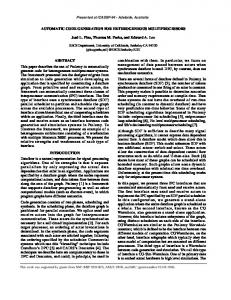
Tensor Expressions TCE Language Parser Simple Expression Tree Optimizations

Figure 1: A general schematic representation of the architecture of the Tensor Contraction Engine software tools (both prototype and optimizing). “Tensor Expressions” and “Generated Code” boxes represent the inputs and outputs of the TCE tools. Dashedline boxes represent one or more optimization modules which act on the simple expression tree or abstract syntax tree representations used within the TCE.

Loop Fuser Simple Code Generator

Abstract Syntax Tree Generator Abstract Syntax Tree Optimizations Code Generator

Generated Code

To date, applications of automatic code-generation ideas in electronic structure theory, and indeed in other areas of computational science as well, have focused essentially on either productivity (increasing the rate at which software can be created) or the performance of the resulting software. However there is no limitation intrinsic to the approach that prevents both goals from being pursued simultaneously. The Tensor Contraction Engine (TCE) is a unique effort to bring together the productivity and performance benefits of automatic code generation to quickly and easily produce high-performance parallel implementations of a broad spectrum of many-body electronic structure methods. The project team brings together a group of quantum chemists and computer scientists and treats the problem very much like the development of an optimizing compiler. In the following sections, we describe overall approach and architecture of the TCE and provide some specific examples of the benefits of this approach in terms of flexibility, productivity, and performance.

9

3

The Tensor Contraction Engine

The Tensor Contraction Engine is structured along the same basic lines as a compiler for a general-purpose language, such as Fortran: an input language is parsed into an internal representation, that internal representation is processed to transform and optimize it, and finally “executable” code is generated. In the case of the TCE, the input language is a high-level, domain-specific language which allows the user to express the equations to be implemented in a form natural to a quantum chemist, based on tensor expressions. The use of a high-level input language provides the TCE with a view of the problem in a natural form of expression, before it is translated to satisfy the constraints of a general-purpose language, such as Fortran. Based on this high-level view, the TCE can perform optimizations that are not possible once the desired operations have been translated into a general-purpose language. These optimizations can rigorously and systematically explore the space of possible transformations, compared to the far more empirical approach typically taken by software developers implementing such codes by hand. Moreover, it is possible to tailor the TCE’s processing and optimizations to the resources and performance characteristics of each hardware platform on which the generated code will run, producing a different implementation tuned to each target system. In fact, the generated code can even be tailored to specific chemical problems, which may be useful for extremely large or complex calculations. Fig. 1 illustrates the overall architecture of the TCE, and the various components shown in the diagram are described in more detail below.

10

3.1 Tensor Expressions and the TCE Language Parser In order to illustrate the operation of the first two boxes in Fig. 1, consider the basic tensor expression Sabij =

X

Aacik Bbef l Cdf jk Dcdel .

(1)

cef kl

This equation might be rendered in the TCE’s input language as shown in Listing 1. All indices appearing in TCE inputs are declared as being associated with a particular range of values (lines 4–5). Ranges must be declared with a size (lines 1–2) to allow the compiler to compute the cost and resource requirements of each expression during the optimizations. These sizes amount to upper bounds – the generated code will work up to the indicated size, but may fail beyond it due to resource exhaustion. TCE procedures are named and declare both their input and output data (lines 9–10). Tensor expressions are written as explicit summations in notation reminiscent of that used by Mathematica [76] (lines 12–13). The mlimit declaration indicates the amount of main memory available on the target system. The TCE input language also allows external (i.e. not generated by the TCE) functions to be declared and used in tensor expressions, for example to obtain integrals. The TCE input is parsed and converted into an expression tree, in which the tensor contraction expressions are represented as a binary tree, with nodes for each operator or summation in the expression and tensor elements (i.e. A[a,c,i,k]) as the leaves. This is the first of two “internal representations” used within the TCE, which can be transformed in systematic ways by various optimizations.

11

1 2

range V = 3000; range O = 100;

3 4 5

index a,b,c,d,e,f : V; index i,j,k,l : O;

6 7

mlimit = 100GB;

8 9 10 11 12 13 14

procedure P(in A[V,V,O,O], in B[V,V,V,O], in C[V,V,O,O], in D[V,V,V,O], out S[V,V,O,O])= begin S[a,b,i,j] == sum[ A[a,c,i,k] * B[b,e,f,l] * C[d,f,j,k] * D[c,d,e,l], {c,e,f,k,l}]; end

Listing 1: TCE input corresponding to Eq. 1.

3.2 Expression Tree Optimizations and Loop Fusion Operation minimization applies transformations based on the algebraic properties of commutativity and associativity of addition and multiplication, and the distributivity of multiplication over addition in order to obtain an equivalent form with the minimal scaling [77,78]. For example, the four-fold contraction of Eq. 1, which is O(o 4 v 5 ) as written, would be transformed to the sequence of pairwise contractions costing O(o2 v 4 + o3 v 3 ) shown in Fig. 2a. This optimization would also convert the usual O(N 8 ) form in which a four-index integral transformation is typically written (as a single contraction involving five factors) into the O(N 5 ) form in which it is usually implemented (a sequence of pairwise contractions). This optimization operates on the expression tree representation of the TCE input, and is represented by the upper dashed box in Fig. 1. At present, these transformations can be applied to all terms within a single statement. We are working to generalize this optimization so that it can work across multiple statements, which will allow recognization of common subexpressions and more effective factorization. Because the operation minimization phase tends to introduce very large intermediate tensors which may exceed the available memory, loop fusion is used next to minimize the space 12

I1bcdf

=

X

Bbef l × Dcdel

X

I1bcdf × Cdf jk

X

I2bcjk × Aacik

el

I2bcjk

=

df

Sabij

=

ck

(a) Formula sequence

S = 0; for b, c  I1=0; I2=0; S=0; I1f = 0; I2f = 0;  for d, f £for b, c, d, e, f, l   I1bcdf += Bbefl Dcdel   £for e, l for b, c, d, f, j, k   £ I1f += Bbefl Dcdel   I2bcjk += I1bcdf Cdfjk   for j, k  £  £for a, b, c, i, j, k I2fjk += I1f Cdfjk  Sabij += I2bcjk Aacik  for a, i, j, k £ (b) Direct implementation (unfused Sabij += I2fjk Aacik code) (c) Memory-reduced implementation (fused)

Figure 2: Example illustrating use of loop fusion for memory reduction based on the tensor contraction in Eq. 1. required for temporaries (also known as memory minimization) [79]. This technique selectively moves loops for the generation of temporary tensors closer to where they are used, so that the temporary can be generated and consumed in subsections instead of having to evaluate the entire tensor, as illustrated in Fig. 2 (notice that in the fused code I1f is a scalar and I2f is rank-2 whereas in the unfused version, both are rank-4). Normally, the loop-fusion optimization would be applied so as to preserve the overall computational cost determined in the operation minimization step, but more aggressive fusion is also possible, with an increase in cost (effectively undoing some or all of the operation minimization). This may be useful, for example, if an important calculation is so large (or resources so constrained) that it cannot fit in the available memory and disk storage, and the user is willing to pay the additional computational cost. Because loop fusion can interact strongly with subsequent optimizations, the loop fuser does not actually try to select the “best” set of loop fusions, but rather annotates the expression tree with information about a set of the highest-ranking fusion options to allow for flexibility later in the optimization process.

13

3.3 Abstract Syntax Tree Generation and Optimizations The expression tree used in the upper part of Fig. 1 is a very simple representation of the desired computations which allows only limited opportunities for optimization. Further optimization requires a more detailed representation in which the individual loops, I/O operations, and other features that must appear in the final generated code can be represented. This representation, known in computer science as an abstract syntax tree (AST) [80], is generated by the TCE from the output of the loop fusion operation. The flexibility of the AST allows a much broader range of optimizations (represented collectively as the lower dashed box in Fig. 1). Similar representations are used within compilers for general-purpose languages, and there are many similar features in the types of optimizations available in general-purpose compilers and those being used in the TCE. An important difference, however, is that TCE optimizations can take advantage of the fact that the problem space is limited to electronic structure methods to perform transformations that would not be applicable in a more general context. At present, the primary optimizations available at this stage of the TCE’s execution are: • Data distribution and partitioning: In order to generate efficient parallel code, attention must be paid to the details of how the data is distributed across the machine. This component seeks distributions of the data that will minimize the parallel communication required to evaluate the tensor equations. Since the data distribution pattern affects the memory usage on the parallel machine, this component is closely coupled with the memory-minimization component [81]. • Space-time transformation: Depending on the method and the size of the chemical 14

problem, the earlier loop-fusion optimization may be able to reduce memory usage so that the entire computation fits into main memory, memory plus available disk space, or it may not even be able to fit the calculation into the available storage at all. In the last case, the calculation cannot be performed unless it is possible to trade storage for recomputation of certain quantities; if the calculation requires the use of disk storage, there may be performance advantages to recomputation instead of storing on disk. The space-time transformation module systematically explores opportunities to trade storage space for recomputation to either fit the problem into available storage, or to improve performance. In the former case, if no satisfactory transformation is found, feedback is provided to the Memory Minimization module, causing it to seek a different solution through more aggressive loop fusion [82]. If the space-time transformation module is successful in bringing down the memory requirement below the disk capacity, the datalocality optimization module is invoked. • Data-locality optimization: On modern computer architectures, the idea of blocking (also known as tiling) a calculation to make effective use of the CPU’s cache memory is widely used to improve performance. Such optimizations are based on maximizing the locality of the computation, so that data can be brought into cache and reused as much as possible before it is evicted. For a disk-based calculation, the computer’s main memory can be treated as the “cache” and the same ideas can be applied to optimizing the movement of data between disk and main memory. The data-locality optimization module determines the optimum tile sizes to obtain the best overall performance from the memory hierarchy [83, 84].

15

3.4 Code Generation Once all desired transformations and optimizations are complete, the output code must be generated. In the case of a general-purpose compiler this would be binary object code, but for simplicity, the TCE produces its output in a general purpose programming language (we have arbitrarily chosen Fortran). The code-generation phase of the TCE is depicted in two places in Fig. 1: the Code Generator at the bottom of the diagram, and the Simple Code Generator near the middle. The Simple Code Generator represents the option to skip the more complex optimizations which act on the detailed abstract syntax tree representation and generate code directly from the expression tree representation. This option reflects the way the TCE has been developed. The longer path, including all possible opportunities for optimization represents the structure of the “optimizing TCE” or o-TCE, while the shorter path represents the structure of the “prototype TCE” or p-TCE. The optimizations of the o-TCE acting on the detailed abstract syntax tree representation are the most complex aspect of the development of the TCE – many of the optimizations currently implemented were newly developed as part of this project. The p-TCE, initially developed by So Hirata [45, 46], provides a simpler environment in which to explore certain aspects of the code generation problem, though of course it lacks much of the optimization capability of the o-TCE. In order for the o-TCE framework to be as extensible as possible, both within the area of many-body methods, and in the longer term beyond it, we are striving to carefully distinguish the origins of various code generation aspects and optimizations possible in many-body methods as arising from the mathematical properties of tensors, the physics of fermionic systems, or the chemical or physical nature of the system being studied, for example.

16

In this respect, the p-TCE has proven very useful in allowing us to systematically capture and explore aspects of automatic code generation for many different electronic structure methods and implementation models without having to worry about the complexity of having fully general AST-based optimizations that will work universally. For either code-generation module, the code being produced must be targeted to a particular environment. This includes how it is interfaced with an existing electronic structure package to obtain the integrals and other inputs required, as well as the specific parallel programming model. At present, we have chosen to focus on NWChem [39, 40] as the electronic structure package (though code generated by the p-TCE has also been interfaced with UTChem [85,86]). For parallel computing, we are using the Global Array Toolkit [87–89], which is widely used in parallel electronic structure packages [39, 90–94]. Since at present, the TCE is only capable of evaluating tensor contraction expressions themselves, the generated code must be wrapped up into a (hand-written) driver to handle the overall sequencing and iteration of the tensor expressions, and we also assume that various numerical and other libraries are available (such as the BLAS). An important feature of this approach is the flexibility provided by the code-generation process. Retargeting the code to interface with a different electronic structure package, parallel programming model, or other variations in the environment is primarily a matter of modifying the code-generation portion of the TCE (though in some cases some optimizations may also need to change). Once the modifications are made to the code generator, an entire range of methods can be generated targeting the new environment. The resulting changes often suffuse the entire code, so hand implementations would require significant modification for each and every method separately. In the following section, we present an example which takes advan17

tage of the flexibility of the code generation approach, as well as examples of some of the other optimizations implemented in the TCE.

4

Examples of TCE Components in Operation

In order to provide further insight into the operation and capabilities of the TCE, in this section we present examples of various modules of the TCE in operation: our algorithm for operation minimization, which is providing results very close to the best known manual CCSD implementation; the effect of loop fusion and data locality optimizations on an out-of-core four-index transformation; and finally, an example of a new parallel CCSD(T) algorithm implemented using the TCE.

4.1 The Operation-Minimization Optimization As discussed in the previous section, transforming the input equations into a form that has the appropriate computational scaling, often known as operation minimization or strength reduction, is one of the most critical optimizations in the TCE. When a method is being implemented by hand, these kinds of transformations are generally made on a largely empirical basis, informed by the developers experience, familiarity with the literature, etc., and tend to evolve and improve slowly over time. In an automatic code-generation environment like the TCE, the power of the computer can be used to perform a much more rigorous (and perhaps even a complete) search of the alternatives for operation minimization or other kinds of optimizations in order to find the best one. Moreover, optimizations in the TCE can easily be applied to the whole range of methods for which the TCE can produce code, while in traditional software 18

development, each method’s implementation would have to be hand optimized separately. Operation minimization acts on the expression-tree representation, which is a straightforward translation of the input equations into a binary tree of variables (i.e. tensor elements) and mathematical operations (i.e. multiplication, addition, summation). The input equations can be transformed into equivalent expressions through algebraic manipulations based on properties such as commutativity, distributivity, associativity, etc. Each variant would give rise to a new expression tree which differs from the original input form only with respect to the specific algebraic manipulations that have been performed on it. Each tree also has a unique cost associated with it based on the number and types of operations to be performed. (For example, A × B + A × C costs 4N 3 + N 2 operations if all matrices are N × N , while A × (B + C) costs 2N 3 + N 2 .) The task of operation minimization is to search among all these equivalent expression trees to find the one with the minimum cost. Unfortunately, the number of alternative representations grows very quickly with the complexity of the input equation, and the optimization is NP-complete [95], meaning that the known algorithms to solve it are exponential in cost, making it infeasible in general to perform an exhaustive search for the minimum. Instead, we use a heuristic algorithm to search for a solution approximating the global-minimum operation cost. To understand the algorithm, consider each of the alternative expression trees above as a single node in a larger graph. Adjacent nodes differ from each other by a single algebraic transformation. Each node has a number of neighbors corresponding to every possible algebraic transformation that can be applied to every element of the tree. A simple search strategy would be to examine all the immediate neighbors of the starting node (i.e. those that differ by exactly one algebraic transformation somewhere in the expression tree) and choose the one 19

with the least cost. The procedure is repeated at the new node, resulting in a direct-descent algorithm. The direct descent algorithm will find a local minimum in the graph, but there is no guarantee of finding the global minimum in this way. An improvement on this algorithm is to perform a number of trials in which the first (or first several) step is taken at random and then direct descent is used from there to find a local minimum. The final result of the algorithm is the minimum over the local minima found in each trial. Preliminary results of applying these search strategies to the CCSD T 2 equations [96, 97] are shown in Table 2. For the “random + descent” search algorithm, we perform 100 trials consisting of a single random step from the input equations followed by direct descent to a local minimum and taking the lowest result from all trials. As we can see, both search algorithms obtain results that are significantly better than the original input form, and the random + descent algorithm obtains a slightly lower coefficient for the o 3 v 2 term. Comparing the search results with the best known manual CCSD formulation by Stanton and coworkers [97], we see that N 6 terms match. In the N 5 terms, the search results are fairly close to those of Stanton et al., but somewhat higher. We consider these preliminary results to be very positive, especially when considering they were obtained with a completely automatic operation-minimization algorithm which uses purely algebraic properties, without chemistry-specific information of any kind. Moreover, the manual result we are comparing with did not appear until fully nine years after the first implementation of the CCSD method appeared [96]. We are now exploring the use of this approach to operation minimization for CC methods with higher excitations, where much less effort has been expended to date in manually minimizing the operation counts. We are also working to enhance the optimization algorithm itself. Currently, it operates across all terms in a single statement, but ultimately it will be able 20

Table 2: Comparison of the costs of various forms of the CCSD T 2 equation. The original input expressions (first line) served as the starting point for the direct-descent and random + descent optimization algorithms described in the text. These results are compared with the best known manual formulation of the equations, by Stanton et al. [97]. o and v are the size of the occupied and virtual orbital spaces, respectively, with o + v = N . Only the leading terms (N 6 and N 5 ) are shown; N 4 and smaller terms are neglected. Equations Original input TCE direct descent TCE random + descent Stanton et al.

N6 1 2 4 ov 4 1 2 4 ov 4 1 2 4 ov 4 1 2 4 ov 4

15 3 3 ov 2 3 3

+ + + 4o v + + 4o3 v 3 + + 4o3 v 3 +

11 4 2 ov 2 1 4 2 ov 2 1 4 2 ov 2 1 4 2 ov 2

4

+ ov + + 2ov 4 + + 2ov 4 + + ov 4 +

N5 + 49 o3 v 2 + 7o4 v 2 8o v + 9o3 v 2 + 3o4 v 8o2 v 3 + 8o3 v 2 + 3o4 v 6o2 v 3 + 10o3 v 2 + o4 v

19 2 3 ov 2 2 3

to work on multiple statements to optimize an entire TCE procedure, or even multiple procedures, adding the capability to recognize and take advantage of common subexpressions across a set of equations. We are also exploring more exhaustive search strategies such as simulated annealing or genetic algorithms.

4.2 Loop-Fusion and Tiling Optimizations for the Four-Index Transformation As an example to illustrate the impact of the loop-fusion and optimized tiling transformations being implemented in the TCE, we consider the AO-to-MO integral transformation (virtual orbitals only).1

B(a, b, c, d) =

X

C(σ, d)C(λ, c)C(ν, b)C(µ, a)A(µ, ν, λ, σ)

µ,ν,λ,σ

1

Since spatial and permutational symmetry are not yet modeled in the o-TCE, the data presented here is for fully dense tensors, but the optimization approach is expected to be similarly effective for the computations that exploit symmetry.

21

where indices a–d denote virtual orbitals and µ–σ denote the full orbital space. The operation-minimal way of computing B would be through the use of four steps, with temporary intermediate tensors I1, I2, and I3, as follows:

I1(a, ν, λ, σ) =

X

C(µ, a)A(µ, ν, λ, σ)

X

C(ν, b)I1(a, ν, λ, σ)

X

C(r, c)I2(a, b, λ, σ)

X

C(s, d)I3(a, b, c, σ)

µ

I2(a, b, λ, σ) =

ν

I3(a, b, c, σ) =

λ

B(a, b, c, d) =

σ

If the integrals are too large to fit in memory, tiling of the loops will be required, so that the tensors are processed in blocks that can fit within memory. A straightforward way of doing this is to directly tile the loops corresponding to each of the four steps, using uniform tile sizes on all dimensions. Thus, the loops for the first step would be tiled with the same tile size t along all indices µ, ν, λ, σ, and a. Due to the rank-4 tensors, the maximum tile size is limited to the order of the fourth root of memory size. Tile sizes may also be optimized individually [98, 99]. The overhead of disk I/O can be reduced by using loop fusion, so that the ranks of some of the intermediate tensors are reduced, allowing them to be completely memory resident to avoid disk I/O (see Fig. 2, Section 3.2, and [98, 99]). While it is impossible to perform loop fusions to reduce the ranks of all three temporaries simultaneously, there are a number of ways of using loop fusion to reduce the ranks of two of the three intermediates. In Table 3 we compare timings for three different implementations of this four-index transformation: 22

Table 3: Total disk I/O and execution times for code generated with the benefit of various optimizations, as described in the text. Results were obtained on a 900 MHz Itanium 2 system with 4 GB of memory (denoted M below), for 140 virtual orbitals and 150 AO orbitals. Optimizations Included and Omitted q No Fusion, Tile size = 4 M3 No Fusion, Optimized Tiling Fusion + Optimized Tiling

Total Disk I/O Total Execution I/O time (s) time (s) 1241 1957 748 1262 248 955

1. No Fusion, Simple Tiling: Neither loop-fusion nor tile-size optimization is enabled; equi-sized tiles along all dimensions are used, based on the 4 th root of the memory size. 2. No Fusion, Optimized Tiling: No loop fusion is used (i.e. all intermediates I1, I2, and I3 are fully produced and written out to disk and then read back to be consumed), but the o-TCE tiling optimization is enabled, so that different combinations of tile sizes are explored and the best chosen. 3. Fusion + Optimized Tiling: The o-TCE loop-fusion and tiling optimizations are used to search amongst a large space of loop structures corresponding to different combinations of loop fusion and tile sizes. It can be seen that the combined use of fusion and tiling optimizations results in code that has 80% less disk I/O than the version with the simple tiling, and a 66% reduction in total execution time.

23

4.3 Code Generation for a Loop-Fused Replicated-Data Parallel CCSD(T) Implementation A long-term goal of the TCE project is, given an accurate performance model for virtually any platform, to be able to generate near-optimal code – automatically taking into account the processor and network performance, memory and disk resources and other features. However since this is not yet possible, we have taken advantage of the code-generation capabilities of the TCE to produce a CCSD(T) [100] implementation designed for the capabilities of modestlysized, low-cost commodity Beowulf cluster computers which are now widely accessible, even in the individual laboratories of many computational chemists. In this section, we outline our on-going work in this area. CCSD(T) has become a “workhorse” method of modern quantum chemistry because it provides a relatively low-cost way of introducing some triple-excitation effects based on a converged CCSD wavefunction. The development of parallel algorithms in which the data (t– amplitudes, integrals, etc.) are fully distributed across the system is extremely complex and finding a highly scalable distributed-data parallel formulation with the TCE is still some ways off. Nevertheless, it would be useful to be able to speed up such calculations using widely available commodity-cluster systems. By replicating the key data across all processes of the parallel computer, we can eliminate much of the complex data communications that would be required for a fully distributed algorithm. Instead we have a single, simple communication phase in each CCSD iteration in which partial contributions to the t–amplitude residuals are summed and the result redistributed to all processes. Loop-fusion techniques are used to insure that the CCSD iteration can take place without the need for additional communication of in-

24

for k < l, i < j £ I2(k,l,i,j) = sum (c