Lecture: Continuous-time linear systems. Automatic Control 1. Continuous-time
linear systems ...... x1(t) = x10 + x20t x2(t) = x20. Note: A is not diagonalizable ! 0.
Lecture: Continuous-time linear systems
Automatic Control 1
Continuous-time linear systems Prof. Alberto Bemporad University of Trento
Academic year 2010-2011
Prof. Alberto Bemporad (University of Trento)
Automatic Control 1
Academic year 2010-2011
1 / 42
Lecture: Continuous-time linear systems
Dynamical systems
Dynamical models
A dynamical system is an object (or a set of objects) that evolves over time, possibly under external excitations. Examples: a car, a robotic arm, a population of animals, an electrical circuit, a portfolio of investments, etc. The way the system evolves is called the dynamics of the system. A dynamical model of a system is a set of mathematical laws explaining in a compact form and in quantitative way how the system evolves over time, usually under the effect of external excitations. Main questions about a dynamical system: 1 2 3
Understanding the system (“How X and Y influence each other ?”) Simulation (“What happens if I apply action Z on the system ?”) Design (“How to make the system behave the way I want ?”)
Prof. Alberto Bemporad (University of Trento)
Automatic Control 1
Academic year 2010-2011
2 / 42
Lecture: Continuous-time linear systems
Dynamical systems
Dynamical models
Qualitative models only useful in non-technical domains (examples: politics, advertisement, psychology,...) Experiments provide an answer, but have limitations: 1 2 3
maybe too expensive (example: launch a space shuttle) maybe too dangerous (example: a nuclear plant) maybe impossible (the system doesn’t exist yet!)
In contrast, mathematical models allows us to: 1
2 3
capture the main phenomena that take place in the system (example: Newton’s law – a force on a mass produces an acceleration) analyze the system (relations among dynamical variables) simulate the system (=make predictions) about how the system behaves under certain conditions and excitations (in analytical form, or on a computer)
Prof. Alberto Bemporad (University of Trento)
Automatic Control 1
Academic year 2010-2011
3 / 42
Lecture: Continuous-time linear systems
Dynamical systems
Dynamical models Working on a model has almost zero cost compared to real experiments (just mathematical thinking, paper writing, computer coding) However, a simulation (or any other inference obtained from the model) is as better as the dynamical model is closer to the real system Conflicting objectives: 1
Descriptive enough to capture the main behavior of the system
2
Simple enough for analyzing the system
“Make everything as simple as possible, but not simpler.” – Albert Einstein Albert Einstein (1879-1955)
Making a good model is an art ! (that you are learning ...) Prof. Alberto Bemporad (University of Trento)
Automatic Control 1
Academic year 2010-2011
4 / 42
Lecture: Continuous-time linear systems
Differential equations
Ordinary differential equations (ODEs) First order differential equation (=the simplest dynamical model): ¨ ˙x(t) = ax(t) a ∈ R, ˙x ¬ dx dt x(0) = x0 x0 ∈ R Its unique solution is x(t) = eat x0 4.5 4 3.5
a>0
x(t)
3 2.5 2 1.5
a=0
1
a t (strictly causal if ∀τ ≥ t) A linear system is always causal, and strictly causal iff D = 0 Linear time-varying (LTV) systems: � ˙x(t) = A(t)x(t) + B(t)u(t) y(t) = C(t)x(t) + D(t)u(t) When A, B, C, D are constant, the system is said linear time-invariant (LTI) Multivariable systems: more generally, a system can have m inputs (u(t) ∈ Rm ) and p outputs (y(t) ∈ Rp ). For linear systems, we still have � ˙x(t) = Ax(t) + Bu(t) y(t) = Cx(t) + Du(t) with A ∈ Rn×n , B ∈ Rn×m , C ∈ Rp×n , D ∈ Rp×m Prof. Alberto Bemporad (University of Trento)
Automatic Control 1
Academic year 2010-2011
23 / 42
Lecture: Continuous-time linear systems
Linear systems
Some classes of dynamical systems
Nonlinear systems �
˙x(t) y(t)
= =
f (x(t), u(t)) g(x(t), u(t))
where f : Rn+m → Rn , g : Rn+m → Rp are (rather arbitrary) nonlinear functions Time-varying nonlinear systems are very general classes of dynamical systems � ˙x(t) = f (t, x(t), u(t)) y(t) = g(t, x(t), u(t))
Prof. Alberto Bemporad (University of Trento)
Automatic Control 1
Academic year 2010-2011
24 / 42
Lecture: Continuous-time linear systems
Stability
Equilibrium Consider the continuous-time nonlinear system � ˙x(t) = f (x(t), u(t)) y(t) = g(x(t), u(t))
Definition A state xr ∈ Rn and an input ur ∈ Rm are an equilibrium pair if for initial condition x(0) = xr and constant input u(t) ≡ ur the state remains constant: x(t) ≡ xr , ∀t ≥ 0
Equivalent definition: (xr , ur ) is an equilibrium pair if f (xr , ur ) = 0 xr is called equilibrium state, ur equilibrium input The definition generalizes to time-varying nonlinear systems Prof. Alberto Bemporad (University of Trento)
Automatic Control 1
Academic year 2010-2011
25 / 42
Lecture: Continuous-time linear systems
Stability
Stability Consider the nonlinear system � ˙x(t) y(t)
= =
f (x(t), ur ) g(x(t), ur )
and let xr an equilibrium state, f (xr , ur ) = 0 Definition The equilibrium state xr is stable if for each initial conditions x(0) “close enough” to xr , the corresponding trajectory x(t) remains near xr for all t ≥ 0 a a
Analytic definition: ∀ε > 0 ∃δ > 0 : kx(0) − xr k < δ ⇒ kx(t) − xr k < ε, ∀t ≥ 0
The equilibrium point xr is called asymptotically stable if it is stable and x(t) → xr for t → ∞ Otherwise, the equilibrium point xr is called unstable Prof. Alberto Bemporad (University of Trento)
Automatic Control 1
Academic year 2010-2011
26 / 42
Lecture: Continuous-time linear systems
Stability
1
1
1
0.8
0.8
0.8
0.6
0.6
0.6
0.4
0.4
0.4
0.2
0.2
0
0.2
x2(t)
x2(t)
x2(t)
Stability of equilibria - Examples
0
0
−0.2
−0.2
−0.2
−0.4
−0.4
−0.4
−0.6
−0.6
−0.6
−0.8
−0.8
−1
−1
−1
−0.8
−0.6
−0.4
−0.2
0
x1(t)
0.2
0.4
0.6
0.8
−0.8 −1
−1
1
−0.8
−0.6
−0.4
−0.2
0
x1(t)
0.2
0.4
0.6
0.8
1
−1
asymptotically stable equilibrium
stable equilibrium 1
0.4 0.2
x2
0
0
x1
0
x2
−2
0.5
dx dt
1
=
�
1.5
2
2.5
3
−2x1 (t) − 4x2 (t) 2x1 (t) + 2x2 (t)
3.5
�
Prof. Alberto Bemporad (University of Trento)
4
−0.8
0
x1(t)
0.2
0.4
0.6
0.8
1
x1
−6
−0.4
0
−0.2
−4
x2
−8
−0.6 −1
−0.4
unstable equilibrium
−0.2 −0.5
−0.6
2
0.6
x1
0.5
−0.8
−10 0
0.5
dx dt
1
=
1.5
�
2
2.5
3
−x1 (t) − 2x2 (t) 2x1 (t) − x2 (t)
Automatic Control 1
3.5
�
4
0
0.2
0.4
dx dt
0.6
=
�
0.8
1
1.2
1.4
1.6
2x1 (t) − 2x2 (t) x1 (t)
1.8
2
�
Academic year 2010-2011
27 / 42
Lecture: Continuous-time linear systems
Stability of continuous-time linear systems
Stability of first-order linear systems Consider the first-order linear system ˙x(t) = ax(t) + bu(t) xr = 0, ur = 0 is an equilibrium pair For u(t) ≡ 0, ∀t ≥ 0, the solution is x(t) = eat x0 The origin xr = 0 is 5
unstable if a > 0
4.5
stable if a ≤ 0
4
3.5
asymptotically stable if a < 0 x(t)
3
a>0
2.5
2
x0
1.5
a=0
1
0
a 0 a Algebraic multiplicity of λi = number of coincident roots λi of det(λI − A). Geometric multiplicity of λi = number of linearly independent eigenvectors vi , Avi = λi vi
The stability properties of a linear system only depend on the real part of the eigenvalues of matrix A Prof. Alberto Bemporad (University of Trento)
Automatic Control 1
Academic year 2010-2011
29 / 42
Lecture: Continuous-time linear systems
Stability of continuous-time linear systems
Stability of continuous-time linear systems Proof: The natural response is x(t) = eAt x0 (eAt ¬ I + At + If matrix A is diagonalizable , A = TΛT 3
λ
1 0 ... 0 λ2 ...
0 0
−1
0 ... λn
+ ... +
An t n n!
+ ...)
,
eλ1 t
0 At Λ= .. .. . . .. ⇒ e = T .. . . . . . 0
A2 t 2 2
0
0 ... eλ2 t ...
0 0
−1 . . . T . .. . . .
0
... eλn t
Take any eigenvalue λ = a + jb: |eλt | = eat |ejbt | = eat A is always diagonalizable if algebraic multiplicity = geometric multiplicity 3 If A is not diagonalizable, it can be transformed to Jordan form. In this case the natural response x(t) contains modes tj eλt , j = 0, 1, . . . , alg. multiplicity - geom. multiplicity Prof. Alberto Bemporad (University of Trento)
Automatic Control 1
Academic year 2010-2011
30 / 42
Lecture: Continuous-time linear systems
Stability of continuous-time linear systems
Example 1 ˙x(t) = solution:
�
x(0) =
0 2
x
x1 (t) x2 (t)
�
= = 1
0.5
0.5
� x(t)
0
−0.5
⇒ eigenvalues of A: {−1, −2}
x10 (2e−t − e−2t ) + x20 (−e−t + e−2t ) x10 (2e−t − 2e−2t ) + x20 (−e−t + 2e−2t )
x2(t)
1
x1(t)
10
x20
−1 −3
asymptotically stable 0
0
2
4
6
8
−0.5
t Prof. Alberto Bemporad (University of Trento)
0
2
4
6
8
t Automatic Control 1
Academic year 2010-2011
31 / 42
Lecture: Continuous-time linear systems
Stability of continuous-time linear systems
Example 2 ˙x(t) =
�
x(0) =
x
10
x20
�
1.5
1.5
1
1
0.5
0.5
x2(t)
x1(t)
solution:
0
−0.5
−1
−1
0
2
4
6
8
10
x(t)
x1 (t) x2 (t)
= =
−1.5
t Prof. Alberto Bemporad (University of Trento)
⇒ eigenvalues of A: {+j, −j}
x10 cos t − x20 sin t x10 sin t + x20 cos t
marginally stable
0
−0.5
−1.5
�
−1 0
0 1
0
2
4
6
8
10
t Automatic Control 1
Academic year 2010-2011
32 / 42
Lecture: Continuous-time linear systems
Stability of continuous-time linear systems
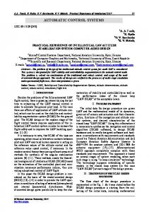
Example 3
�
˙x(t) = x(0) =
solution: �
x1 (t) x2 (t)
= =
0 0
x
10 x20
1 0
� x(t)
⇒ eigenvalues of A: {0, 0}
x10 + x20 t x20
12
2
10
1.5
Note: A is not diagonalizable !
8 1 6
x2(t)
4
1
x (t)
0.5
2
unstable
0
−0.5 0 −1 −2 −1.5
−4
−6
0
2
4
6
8
10
−2
0
t Prof. Alberto Bemporad (University of Trento)
2
4
6
8
10
t Automatic Control 1
Academic year 2010-2011
33 / 42
Lecture: Continuous-time linear systems
Stability of continuous-time linear systems
Example 4 ˙x(t) = x(0) =
solution:
¨
10
x20
10
8
6
6
4
4
2
2
−2
−4
−4
−6
−6
−10
� x(t)
= =
⇒ eigenvalues of A: {−1, 1}
x10 et 1 x et + (x20 − 21 x10 )e−t 2 10
unstable
0
−2
−8
0 −1
x1 (t) x2 (t)
8
0
1 1
x
10
x2(t)
x1(t)
�
−8
0
2
4
6
8
10
−10
0
t Prof. Alberto Bemporad (University of Trento)
2
4
6
8
10
t Automatic Control 1
Academic year 2010-2011
34 / 42
Lecture: Continuous-time linear systems
Linearization
Linearization of nonlinear systems Consider the nonlinear system � ˙x(t) y(t)
= =
f (x(t), u(t)) g(x(t), u(t))
Let (xr , ur ) be an equilibrium, f (xr , ur ) = 0 Objective: investigate the dynamic behaviour of the system for small perturbations ∆u(t) ¬ u(t) − ur and ∆x(0) ¬ x(0) − xr . The evolution of ∆x(t) ¬ x(t) − xr is given by ˙ ∆x(t) = ˙x(t) − ˙xr = f (x(t), u(t)) = f (∆x(t) + xr , ∆u(t) + ur ) ∂f ∂f ≈ (xr , ur ) ∆x(t) + (xr , ur ) ∆u(t) |∂ x {z } |∂ u {z } A
Prof. Alberto Bemporad (University of Trento)
B
Automatic Control 1
Academic year 2010-2011
35 / 42
Lecture: Continuous-time linear systems
Linearization
Linearization of nonlinear systems
Similarly ∆y(t) ≈
∂g ∂g (xr , ur ) ∆x(t) + (xr , ur ) ∆u(t) ∂ x ∂ | {z } | u {z } C
D
where ∆y(t) ¬ y(t) − g(xr , ur ) is the perturbation of the output from its equilibrium The perturbations ∆x(t), ∆y(t), and ∆u(t) are (approximately) ruled by the linearized system � ˙ ∆x(t) = A∆x(t) + B∆u(t) ∆y(t) = C∆x(t) + D∆u(t)
Prof. Alberto Bemporad (University of Trento)
Automatic Control 1
Academic year 2010-2011
36 / 42
Lecture: Continuous-time linear systems
Linearization
Lyapunov’s indirect method Consider the nonlinear system ˙x = f (x), with f differentiable, and assume x = 0 is equilibrium point (f (0) = 0) ∂f Consider the linearized system ˙x = Ax, with A = ∂ x x=0
If ˙x = Ax is asymptotically stable, then the origin x = 0 is also an asymptotically stable equilibrium for the nonlinear system (locally) If ˙x = Ax is unstable, then the origin x = 0 is an unstable equilibrium for the nonlinear system If A is marginally stable, nothing can be said about the stability of the origin x = 0 for the nonlinear system
Aleksandr Mikhailovich Lyapunov (1857-1918) Prof. Alberto Bemporad (University of Trento)
Automatic Control 1
Academic year 2010-2011
37 / 42
Lecture: Continuous-time linear systems
Linearization
Example: Pendulum
l y(t) h m u(t) = mg
y(t) = angular displacement ˙y(t) = angular velocity ¨y(t) = angular acceleration u(t) = mg gravity force h˙y(t) = viscous friction torque l = pendulum length ml2 = pendulum rotational inertia
mathematical model ml2 ¨y(t) = −lmg sin y(t) − h˙y(t) in state-space form (x1 = y, x2 = ˙y) ¨ ˙x1 = x2 g ˙x2 = − l sin x1 − Hx2 ,
Prof. Alberto Bemporad (University of Trento)
Automatic Control 1
H¬
h ml2
Academic year 2010-2011
38 / 42
Lecture: Continuous-time linear systems
Linearization
Example: Pendulum Look for equilibrium states: � � � x2r 0 x2r = 0 = ⇒ g − l sin x1r − Hx2r 0 x1r = ±kπ, k = 0, 1, . . . u(t) = mg h m l l h m u(t) = mg
x2r = 0, x1r = 0, ±2π, . . .
Prof. Alberto Bemporad (University of Trento)
x2r = 0, x1r = 0, ±π, ±3π, . . .
Automatic Control 1
Academic year 2010-2011
39 / 42
Lecture: Continuous-time linear systems
Linearization
Example: Pendulum Linearize the system around x1r = 0, x2r = 0 0 1 ∆˙x(t) = ∆x(t) g − l −H | {z } A
find the eigenvalues of A 2
det(λI − A) = λ + Hλ +
g l
= 0 ⇒ λ1,2 =
1
Ç H2
−H ±
2
−4
g
l
1.5
ℜλ1,2 < 0 ⇒ ˙x = Ax asymptotically stable
1
by Lyapunov’s indirect method � � xr = 00 is also an asymptotically stable equilibrium for the pendulum
y(t)
0.5 0 −0.5 −1 −1.5 0
2
4
6
8
10
t Prof. Alberto Bemporad (University of Trento)
Automatic Control 1
Academic year 2010-2011
40 / 42
Lecture: Continuous-time linear systems
Linearization
Example: Pendulum Linearize the system around x1r = π, x2r = 0 0 1 ∆˙x(t) = g ∆x(t) −H l | {z } A
find the eigenvalues of A 2
det(λI − A) = λ + Hλ −
g l
= 0 ⇒ λ1,2 =
1 2
Ç H2
−H ±
+4
g
l
4 3 2
λ1 < 0, λ2 > 0 ⇒ ˙x = Ax unstable y(t)
by Lyapunov’s indirect method � � xr = 00 is also an unstable equilibrium for the pendulum
1 0 −1 −2 −3 −4 0
2
4
6
8
10
t Prof. Alberto Bemporad (University of Trento)
Automatic Control 1
Academic year 2010-2011
41 / 42
Lecture: Continuous-time linear systems
Linearization
English-Italian Vocabulary
dynamics natural response eigenvalue eigenvector modulus or magnitude angle or phase nonlinear systems controllable canonical form observable canonical form
dinamica risposta libera autovalore autovettore modulo fase sistemi non lineari forma canonica di raggiungibilità forma canonica di osservabilità
Translation is obvious otherwise.
Prof. Alberto Bemporad (University of Trento)
Automatic Control 1
Academic year 2010-2011
42 / 42