Automatic Detection of Floating-Point Exceptions - Earl Barr

Automatic Detection of Floating-Point Exceptions Earl T. Barr

Thanh Vo

Vu Le

Zhendong Su

Department of Computer Science, University of California at Davis {etbarr, vo, vmle, su}@ucdavis.edu

Abstract It is well-known that floating-point exceptions can be disastrous and writing exception-free numerical programs is very difficult. Thus, it is important to automatically detect such errors. In this paper, we present Ariadne, a practical symbolic execution system specifically designed and implemented for detecting floating-point exceptions. Ariadne systematically transforms a numerical program to explicitly check each exception triggering condition. Ariadne symbolically executes the transformed program using real arithmetic to find candidate real-valued inputs that can reach and trigger an exception. Ariadne converts each candidate input into a floating-point number, then tests it against the original program. In general, approximating floating-point arithmetic with real arithmetic can change paths from feasible to infeasible and vice versa. The key insight of this work is that, for the problem of detecting floating-point exceptions, this approximation works well in practice because, if one input reaches an exception, many are likely to, and at least one of them will do so over both floating-point and real arithmetic. To realize Ariadne, we also devised a novel, practical linearization technique to solve nonlinear constraints. We extensively evaluated Ariadne over 467 scalar functions in the widely used GNU Scientific Library (GSL). Our results show that Ariadne is practical and identifies a large number of real runtime exceptions in GSL. The GSL developers confirmed our preliminary findings and look forward to Ariadne’s public release, which we plan to do in the near future. Categories and Subject Descriptors D.2.3 [Software Engineering]: Coding Tools and Techniques; D.2.4 [Software Engineering]: Software/Program Verification — Reliability, Validation; D.2.5 [Software Engineering]: Testing and Debugging — Symbolic execution; F.3.1 [Logics and Meanings of Programs]: Specifying and Verifying and Reasoning about Programs General Terms Algorithms, Languages, Reliability, Verification Keywords Floating-point exceptions; symbolic execution

1.

Introduction

On June 4, 1996, the European Space Agency’s Ariane 5 rocket veered off course and self-destructed because the assignment of a floating-point number to an integer caused an overflow [40]. The loss is estimated to have been US$370 million. Scientific results increasingly rest on software that is usually numeric and

Permission to make digital or hard copies of all or part of this work for personal or classroom use is granted without fee provided that copies are not made or distributed for profit or commercial advantage and that copies bear this notice and the full citation on the first page. To copy otherwise, to republish, to post on servers or to redistribute to lists, requires prior specific permission and/or a fee. POPL’13, January 23–25, 2013, Rome, Italy. Copyright © 2013 ACM 978-1-4503-1832-7/13/01. . . $15.00

may invalidate results when buggy [33]. In February 2010, Toyota implicated control software in its spate of brake failures [3]. Haptic controllers are being used for remote surgery [36]. Numerical software, which uses floating-point arithmetic, is prominent in critical control systems in devices in national defense, transportation, and health care. Clearly, we are increasingly reliant on it. Floating-point numbers are a finite precision encoding of real numbers. Floating-point operations are not closed and may throw exceptions: their result may have an absolute value greater than the largest floating-point number and overflow; it may be nonzero and smaller than the smallest nonzero floating-point number and underflow; or it may lie between two floating-point numbers, require rounding, and be inexact. Dividing-by-zero and the invalid application of an operation to operands outside its domain, like taking the square root of a negative number, also generate exceptions. The IEEE 754 standard defines these exceptions [24]. Writing numerical software that does not throw floating-point exceptions is difficult [19, 22]. For example, it is easy to imagine writing if (x != y){ z = 1 / (x-y); } and then later contending with the program mysteriously failing due to a spurious Divide-by-Zero [19]. As another example, consider a straightforward implementation to compute the 2-norm of a vector [22, 23]: sum = 0; for (i = 0; i < N; i++) sum = sum + x[i] * x[i]; norm = sqrt(sum);

For many slightly large or small vector components, this code may overflow or underflow when evaluating x[i]*x[i] or adding the result to sum. In spite of exceptions during its computation, the norm itself may, nonetheless, be representable as an unexceptional floating-point number. Even when some exceptions are caught and handled, others may not be; these are uncaught exceptions. The Divide-by-Zero in the first example is an uncaught exception. Symbolic analysis has been successfully used to test and validate software [7, 18, 38]. However, little work has considered symbolic analysis of floating-point code, although much work has pursued formalizing IEEE floating-point standards in various proof systems such as Coq, HOL, and PVS. One natural approach is to equip a satisfiability modulo theory (SMT) solver with a theory for floatingpoint. This has proved to be a challenging problem; ongoing efforts simplify and deviate from the IEEE floating-point standard [37]. For detecting floating-point exceptions, our core insight is that, if an exception can occur at a particular operation, then that exception defines a neighborhood in which exception-triggering inputs are numerous. If one of these inputs triggers the exception over the reals, then another is likely to do so over floating-point arithmetic. Guided by this insight, we propose to symbolically execute a numeric program over the reals to search for an exception-triggering input. To this end, we transform a numeric program to explicitly check the operands of each floating-point operation before executing it. If a check fails, the transformed program signals the floating-

point exception that would have occurred if the guarded operation had executed, then terminates. In the transformed program, the constraints are over real, not floating-point numbers, so we can directly feed them into an SMT solver equipped with the theory of reals, such as Microsoft’s Z3 [9]. If we can reach any of these injected program points, we can query the SMT solver for an input that triggers that exception. This input is unlikely to be a floatingpoint number, so we search the neighborhood of that input for a candidate floating point number that also triggers the exception over real arithmetic. To undo the inaccuracy of symbolic execution over the reals, we then test that candidate against the original program, concretely executed over floating-point arithmetic. Our approach, which we have christened Ariadne, automatically detects floating-point exceptions. While not all exceptions are bugs, the utility of Ariadne rests on three observations: 1) over- and underflows can be disastrous, as the loss of the Ariane 5 demonstrates; 2) the GSL developers confirmed as bugs several of the exceptions Ariadne found; and 3) Invalid and Divide-by-Zero exceptions are likely to be bugs. Ariadne reports only real exceptions: when it reports inputs that cause a program to throw a particular floatingpoint exception, that program run on those inputs will certainly throw that exception. When Ariadne finds an exception, developers can use the inputs to fix the bug and to construct a test case to add to their test suite. To realize Ariadne, we extended the symbolic execution engine KLEE [7] to use Z3 (version 3.1) as its SMT solver instead of STP [16], which does not support the theory of reals. Interesting numeric code often results in multivariate, nonlinear constraints. In particular, the constraints we encountered while analyzing the GNU Scientific Library, were usually multivariate and nonlinear (Section 5). We fed these constraints to iSAT, the state of the art nonlinear SMT solver [13], but it only handled less than 1%, rejecting most of our constraints because they contain large constant values that exceed iSAT’s bounds. We also directly gave them to Z3, which had recently added support for multivariate, nonlinear constraints but it could only handle a small percentage. These results motivated us to devise a novel, practical method for handling nonlinear constraints involving rational functions (to support division), which we also incorporated into KLEE; this method works effectively over the constraints arising in our problem setting. A new algorithm for solving nonlinear constraints, realized in a prototype called nlsat, was developed concurrently with our work and added to Z3 [25]. We ran nlsat on 10, 000 of our constraints, uniformly selected at random, and compared its performance to that of our solver, Z3-A RIADNE (Section 5). Z3-A RIADNE resolved 9, 119 of the constraints (5, 510 being satisfiable), while nlsat resolved 5, 248 of the constraints, and returned unknown, timed out, or had parse errors on the rest. Our contributions follow: • The insight that, for the problem of detecting floating-point ex-

ceptions, real arithmetic can effectively model floating-point arithmetic, since when one input triggers a floating-point exception, many are likely to do so and, of those, some will do so over both real and floating-point arithmetic; • An LLVM and KLEE-based implementation of our technique

and its evaluation on the GNU Scientific Library (GSL); • A tool that automatically converts fixed precision numeric

code into arbitrary precision numeric code to detect potentially avoidable overflows and underflows; and

1 2 3

double av1(double x, double y) { return (x+y)/2.0; }

5 6 7

double av2(double x, double y) { return x/2.0 + y/2.0; }

9 10 11

double av3(double x,double y) { return x + (y-x)/2.0; }

13 14 15

double av4(double x, double y) { return y + (x-y)/2.0; }

17 18 19 20 21 22 23 24 25 26 27 28 29 30 31 32 33 34 35 36 37

double average(double x, double y) { int samesign; if ( x >= 0 ) { if (y >=0) samesign = 1; else samesign = 0; } else { if (y >= 0) samesign = 0; else samesign = 1; } if ( samesign ) { if ( y >= x) return av3(x,y); else return av4(x,y); } else return av1(x,y); }

Figure 1: Sterbenz’ average function. functions. Across the 467 functions we analyzed, our tool discovered inputs that generated 2091 floating-point exceptions. 91.9% of these are Underflows and Overflows, while the remainder are Divide-byZero and Invalid exceptions. Some of these exceptions are highly nontrivial, as a particular Divide-by-Zero we describe in detail in Section 5.2 illustrates. We reported preliminary results to the GSL community; they confirmed that our warnings were valid and look forward to the public release of our tool. These results show that modeling floating-point numbers as reals to find exceptions is a sweet spot in the trade-off between practicality and precision. To motivate and clarify our problem, Section 2 presents and explains numerical code that contains floating-point exceptions. We open Section 3 with terminology, then describe the two transformations on which Ariadne rests: the first reifies the exceptions a floating-point operation may throw into program points and the second symbolically handles external functions. We close Section 3 with the algorithms we use to solve multivariate, nonlinear constraints. Section 4 describes the realization of Ariadne. In Section 5, we present the results of analyzing the GSL special functions with Ariadne. We discuss closely related work in Section 6 and conclude in Section 7.

• A practical method for handling nonlinear constraints involving

rational functions over the reals. We evaluated our tool on the GNU Scientific Library (GSL) version 1.14. We analyzed all functions in the GSL that take scalar inputs, which include elementary and many differential equation

2.

Illustrative Example

Floating-point arithmetic is unintuitive. Sterbenz [39] illustrates this fact by computing x+y 2 , the average of two numbers. Even for a “simple” function like this, it requires considerable knowledge to

1 2 3 4 5 6 7 8 9 10 11 12 13 14 15 16

int gsl_sf_bessel_Knu_scaled_asympx_e( const double nu, const double x, gsl_sf_result * result ) { /* x >> nu*nu+1 */ double mu = 4.0*nu*nu; double mum1 = mu-1.0; double mum9 = mu-9.0; double pre = sqrt(M_PI/(2.0*x)); double r = nu/x; result->val = pre * (1.0 + mum1/(8.0*x) + mum1*mum9/(128.0*x*x)); result->err = 2.0 * GSL_DBL_EPSILON * fabs(result->val) + pre * fabs(0.1*r*r*r); return GSL_SUCCESS; }

Figure 2: A function from GSL’s special function collection. implement it well. The four functions av1–4 in Figure 1 are a few possible average formulas. They are all equivalent over the reals, but not over floating-point numbers. For instance, av1 overflows when x and y have the same sign and are sufficiently large, and av2 is inaccurate and requires a second expensive division. Sterbenz performs a very interesting analysis of this problem and defines average that uses av1, av3, and av4 according to the signs of the inputs x and y. Sterbenz proved average to be free of overflows. Our tool Ariadne explores all the paths in average and does not find any overflows, as expected. To run Ariadne, we issue “ariadne sterbenz.c” at the command line to compile and apply the operand checking, explicit floating-point exception transformation, then symbolically execute the result to produce sterbenz.out, which contains the analysis results. Ariadne discovers 6 underflows, reporting, for example x = -3.337611e-308 and y = 2.225074e-308, as an input pair that triggers this exception at line 2. We close with a function that contains each of the four floatingpoint exceptions Ariadne detects, drawn from our test corpus, the GSL special functions. Figure 2 contains the GSL’s implementation of gsl_sf_bessel_Knu_scaled _asympx_e. Run on this function, Ariadne reports that the square-root operation at line 8 throws an Invalid exception when x < 0 and a Divide-by-Zero when x = 0. When nu = -5.789604e+76 and x = 2.467898e+03, the evaluation of mum1*mum9 at lines 10–11 overflows. Finally, when nu = -7.458341e-155 and x = 2.197413e+03, the evaluation of mu = 4.0*nu*nu at line 5 underflows.

3.

Approach

Figure 3 depicts the architecture of Ariadne, which has two main phases. Phase one transforms an input numeric program into a form that explicitly checks for floating-point exceptions before each floating-point operation and, if one occurs, throws it and terminates execution. The transformed program contains conditionals, such as x > DBL_MAX, that cannot hold during concrete execution, where DBL_MAX denotes the maximum floating-point value. The transformed program, including its peculiar conditionals, are amenable to symbolic execution and any program point that symbolic execution reaches without throwing an exception has the property that none of its floating-point variables contain a special value, such as NaN (Not a Number) or ∞. Thus, the numeric constraints generated during symbolic execution involve those floating-point values that are a subset of R and suitable input to an SMT solver supporting the theory of reals. During phase two, Ariadne symbolically executes the transformed program, and for each path that reaches a floating-point exception injected in phase one, it attempts to solve the corresponding path constraint. If a satisfying assignment is found, Ariadne

Exception

Example

Default Result

Overflow Underflow Divide-by-Zero Invalid Inexact

|x + y| > Ω |x/y| < λ x/0 √ 0/0, 0 × ∞, −1 nearest(x op y) 6= x op y

±∞ Subnormals ±∞ NaN Rounded result

Table 1: Floating-point exceptions; x, y ∈ F [23, §2.3]. attempts to trigger the exception in the original code. If it succeeds, Ariadne reports the assignment as a concrete input that triggers the exception. Our symbolic execution is standard; the key challenge in its realization is how to effectively solve the collected numerical constraints, many of which are multivariate, nonlinear. We first present pertinent background in numerical analysis and introduce notation (Section 3.1), then describe our transformation (Section 3.2) and how we solve numerical constraints (Section 3.3). 3.1

Background and Notation

Four integer parameters define a floating-point number system F ⊂ R: the base (radix) β , the precision t, the minimum exponent emin , and the maximum exponent emax . With these parameters and the mantissa m ∈ Z and the exponent e ∈ Z, F = { ±mβ e−t | (0 ≤ m ≤ β t − 1 ∧ emin ≤ e ≤ emax ) ∨ (0 < m < β t−1 ∧ e = emin ) } The floating-point numbers for which β t−1 ≤ m ≤ β t ∧ emin ≤ e ≤ emax holds are normal; the numbers for which 0 ≤ m < β t−1 ∧ e = emin holds are subnormal [23, §2.1]. Ω = β emax (1−β −t ) denotes the maximum floating-point number; −Ω, the minimum. λ = β emin −1 is the smallest normalized floating-point number; æ = β emin −t is the smallest denormalized. Floating-point operations can generate exceptions shown in Table 1. Some applications of the operations on certain operands are undefined and cause the Divide-by-Zero and Invalid exceptions. Finite precision causes the rest. Inexact occurs frequently [19, 26] and is often an unavoidable consequence of finite precision. For example, when dividing 1.0 by 3.0, an Inexact exception occurs because the ratio 1/3 cannot be exactly represented as a floatingpoint number. For this reason, Ariadne focuses on discovering Overflow, Underflow, Invalid, and Divide-by-Zero exceptions. Throughout this section, we abuse Q to denote its arbitrary precision subset. Let fp : Q → F convert a rational into the nearest floating-point value, rounding down. For next : F × F → F, next(x, y) returns the floating-point number next to x in the direction of y. To model path constraints, we consider formulas φ in the theory of reals. For a formula φ , fv(φ ) =~x denotes the free variables in φ . We use S to denote satisfiable or SAT; S¯ to denote unsatisfiable or UNSAT; and U for UNKNOWN. Below, we define algorithms that return satisfying bindings to variables or UNSAT or UNKNOWN. ¯ For this purpose, we define AnF = (V × F)n ] {S,U} to be a disjoint union that is either an n length vector of simultaneous assignments over F to the variables V , or is UNSAT or UNKNOWN. For IS SAT: ¯ An → B, IS SAT(a) returns true if a ∈ / {S,U}. F

3.2

Program Transformation

We first define T , the term rewriting system we use to inject explicit floating-point exception handling into numeric code. For simplicity of presentation, we assume that nested arithmetic expressions have been flattened. We assume that the program terminates after throwing a floating-point exception.

Input Code (C, C++, Fortran)

Symbolic Execution

Input Code + Explicit FP Exceptions

Reify FP Exceptions

Constraints Over ℝ

Exception Triggering Inputs

SMT Solver

Figure 3: The architecture of Ariadne. 3.2.1

Basic Arithmetic Operations

The operator ∈ {+, −, ∗}, and variables x and y bind to floatingpoint expressions. We have the following local rewriting rules:

T (x y)

=

T (x / y)

=

  Overflow if |x y| > Ω Underflow if 0 < |x y| < λ  x y otherwise  Invalid if x = 0 ∧ y = 0     Divide-by-Zero if x 6= 0 ∧ y = 0 Overflow if |x| > |y|Ω   Underflow if 0 < |x| < |y|λ   x/y otherwise

We also have a global contextual rewriting rule T (C[e]) = C[T (e)], where e denotes an expression of the form x y or x / y, and C[·] denotes a program context. Ignoring time-dependent behavior, it is evident that JpK = JT (p)K when the numeric program p terminates without throwing a floating-point exception, where J·K denotes the semantics of its operand. Figure 4a shows a concrete example of how T , specialized to C, transforms a subtraction expression (line 6 of example in Figure 2). The result of the subtraction is checked and, if an exception could occur, execution terminates. The division transformation, depicted in Figure 4b, is the most involved transformation. The original expression is taken from line 9 of the example in Figure 2. A floatingpoint division operation can throw four distinct exceptions, each of which the transformed code explicitly checks. For instance, given the inputs nu = 0.0 and x = 0.0, the original expression would have terminated normally and returned NaN, but the transformed code would detect and output an Invalid exception, then terminate. 3.2.2

Elementary Mathematical Functions

Calls into an unanalyzed library usually terminate symbolic execution. Calls to elementary mathematical functions, such as sqrt, log, exp, cos, sin and pow, are frequent in our constraints. These functions are often handled in hardware, like sqrt. We next describe simple, yet effective, transformations to deal with these functions. Indeed, during our experiments, these transformations enabled us to find approximately 41% of the floating-point exceptions we report. When all of an elementary function’s operands are within its domain, these well-tested, ubiquitous functions do not return specials. To handle an unanalyzed elementary function, therefore, we insert checks that its operands are in its domain and signal the appropriate exception if a check fails, then bind a fresh symbolic variable to the call. These symbolic variables are dependent, since they depend on other symbolic variables. Input symbolic variables are independent. We add the obvious constraints on the range of dependent variables. For instance, we add the constraint d 2 = x, for sqrt, which

1 2 3 4 5 6 7 8 9 10 11

double z = mu - 1.0; double abs1 = fabs(z); if (DBL_MAX < abs1) { perror("Overflow!\n"); exit(1); } if (0 < abs1 && abs1 < DBL_MIN) { perror("Underflow!\n"); exit(1); } double mum1 = z;

1 2 3 4 5 6 7 8 9 10 11 12 13 14 15 16 17 18 19

if (x == 0) { // denominator is zero if (nu == 0) { perror("Invalid!\n"); } else { perror("DivZero!\n"); } exit(1); } double abs1 = fabs(nu); double abs2 = fabs(x); if (abs1 > abs2 * DBL_MAX) { perror("Overflow!\n"); exit(1); } if (0 < abs1 && abs1 < abs2 * DBL_MIN) { perror("Underflow!\n"); exit(1); } double r = nu/x;

(a) Subtraction (line 6 of example in Figure 2).

(b) Division (line 9 of example in Figure 2).

Figure 4: Ariadne transformations realized in C: Ariadne symbolically executes this code over arbitrary precision rationals, where the conditionals can be tested; fabs returns the absolute value of a double. has a polynomial representation, as shown in Figure 5. On line 8 of the example in Figure 2, we replace the call to sqrt with the fresh symbolic variable d and add the constraint d 2 = M_PI/(2.0 ∗ x). A dependent symbolic variable can depend on another dependent variable, as when log(log(x)) is encountered. Dependent variables allow us to defer a call’s evaluation until that variable appears in a path constraint that we feed to the solver. The binding of a dependent variable to a function call is recorded in a table, for use during its evaluation, when we concretize a dependent variable and the variables on which it depends (Section 3.3.1). Table 2 shows the contents of the dependent symbolic variable table when the

 T (sqrt(x))

=

T (exp(x))

=

T (log(x))

=

T (cos(x)) T (sin(x))

= =

T (pow(x, y))

=

Invalid d, where d · d = x

if x < 0 otherwise

  Overflow if x > log(Ω) Underflow if x < log(λ )  d otherwise  Invalid if x ≤ 0 d otherwise d d 

where − 1 ≤ d ≤ 1 where − 1 ≤ d ≤ 1 Invalid d

if x = 0 ∧ y ≤ 0 otherwise

Figure 5: Rewriting rules for elementary mathematical functions. Dependent variable

Expression

d0 d1

sin( xy ) log(x2 + 1x )

Table 2: A dependent symbolic variable table. transformation encounters sin( xy ) and log(x2 + 1x ), which use the independent variables x, y. In Figure 5, we rewrite calls to pow to throw Invalid if its operands are outside its domain. Our rewriting of pow could make additional checks for exceptions, such as y > 0 ∧ ylog(x) > log(Ω), but we found the described handling of pow and the other elementary functions to be very effective over the functions we analyzed. 3.3

Solving Numeric Constraints

Designing SMT solvers that can effectively support multivariate, nonlinear constraints over the reals is an active area of research. Offthe-shelf SMT solvers focus on linear constraints and do not support general nonlinear constraints over the real domain because linear constraints are prevalent in integer programs and solving nonlinear constraints is very expensive (although decidable over the reals). However, real-world numeric applications contain many nonlinear constraints. In our experiment over the GSL special functions, 81% of queries are nonlinear, 73% are multivariate and 62% are both nonlinear and multivariate. Algorithm 1 is the Ariadne solver for floating-point exceptions. During symbolic execution, it is called to solve the numeric path constraints to the program points that represent exceptions, injected during the program transformation (Section 3.2). In addition to the path constraint φ , the Ariadne exception solver takes T , the dependent symbolic variable table built during the transformation phase (Section 3.2.2), p, the original, untransformed numeric program itself, the possible exception e, and l, the location (program point) in p of the operation that may throw e. To solve φ , Algorithm 1 first checks whether φ contains any multivariate numerical constraints. It it does, Algorithm 1 concretizes φ using T to convert φ into a univariate formula. On line 5, it calls the CONCRETIZE method, which interacts with the underlying SMT solver to bind variables that appear in multivariate numeric constraints to values in F (Section 3.3.1); it returns φc with the selected variables replaced with concrete values and ~ac , which records those variable to value bindings. Algorithm 1 calls SOLVE U NIVARIATE (Algorithm 2) to solve a univariate formula. When SOLVE U NIVARIATE finds a satisfying assignment, Algorithm 1 returns the bindings from the calls to both CONCRETIZE

Algorithm 1 ARIADNE S OLVE: Φ × T × P × E × N → AnF solves a numeric path constraint over the reals. This topmost algorithm handles formulae that contain multivariate numerical constraints. When φ contains such a constraint, the solver tries various concretizations up to its MAX_CONCRETIZATIONS bound. Note that n = |fv(φ )|, for φ ∈ Φ. inputs φ ∈ Φ, a numeric constraint from p. T ∈ T, a table of dependent symbolic variables. p ∈ P, the numeric program under analysis. e ∈ E, the potential exception. l ∈ N, the location of e. IS M ULTIVARIATE : Φ → B returns true when passed a formula that contains a multivariate numerical constraint. 1: if ¬IS M ULTVARIATE(φ ) ∧ |T | = 0 then 2: return SOLVE U NIVARIATE(φ , hi, p, e, l) // Algorithm 2 3: else 4: for 1..MAX_CONCRETIZATIONS do 5: φc ,~ac := CONCRETIZE(φ , T ) // Algorithm 3 6: ~a := SOLVE U NIVARIATE(φc ,~ac , p, e, l) // Algorithm 2 7: if IS SAT(~a) then 8: return ~a 9: end if 10: end for 11: return U // Return UNKNOWN. 12: end if

Algorithm 2 SOLVE U NIVARIATE: Φ × AnF × P × E × N → AnF linearizes nonlinear univariate constraints in φ , finds a floating-point solution to the resulting constraints, then checks whether a satisfying solution triggers the given exception at the specified location. inputs φ ∈ Φ, a formula whose numeric constraints are univariate. ~ac ∈ AnF , the concretized bindings. p ∈ P, the numeric program under analysis. e ∈ E, the potential exception. l ∈ N, the location of e. 1: φ 0 := LINEARIZE(φ ) // Algorithm 4 2: ~a := ~ac + SOLVE OVERF(φ 0 ) // Algorithm 5 3: if IS SAT(~a) ∧ p(~a) does not throw e at l then 4: return U // Return UNKNOWN. 5: end if 6: return ~a

and SOLVE U NIVARIATE. Algorithm 1 tries different concretizations up to MAX_CONCRETIZATIONS times. Our experiments validate our core insight that, if an exception is reachable, many inputs reach it: varying MAX_CONCRETIZATIONS did not greatly change Ariadne’s detection rate (See Section 5.1). To convert a nonlinear univariate formula into a linear formula, Algorithm 2 applies a linearization technique that finds the roots of each nonlinear polynomial constraint, then rewrites the constraints into an equivalent disjunction of interval checks (Section 3.3.2). When φ is linear, φ 0 = φ . While φ 0 is univariate and linear upon input to SOLVE OVERF on line 2, it remains a formula in the theory of reals, so the underlying SMT solver, used in CONCRETIZE in Algorithm 1 and here in the SOLVE OVERF function, may return a solution in Q \ F. The SOLVE OVERF algorithm (Section 3.3.3) finds a floating-point solution in Fn for its input, if one exists. The SOLVE OVERF function’s solution reaches and triggers an exception when symbolically executed using real arithmetic, but may not when concretely executed using floating-point arithmetic. For instance, consider “if(x + 1 > Ω) Overflow”. The binding x = Ω is valid solution in the theory of reals and SOLVE OVERF can return

it, since x ∈ F. Under concrete execution with standard floating-point semantics, however, the difference in magnitude of the operands means that the result of the addition operation must be truncated to fit into the finite precision of floating-point which “absorbs” the 1 into x’s value of Ω. Under floating-point arithmetic, this Overflow is unreachable and the binding produced during symbolic execution is a false positive. Approximating floating-point arithmetic with real arithmetic can also produce false negatives, again due to rounding. Thus, each satisfying solution SOLVE OVERF produces is a candidate solution that Ariadne must concretely check. In Algorithm 2, line 3 performs the requisite concrete check over floating-point. Here, the Ariadne exception solver executes p on the candidate satisfying assignments — both those found by SOLVE OVERF and ~ac from concretization — to determine whether p actually throws the e at l, the location of the floating-point operation under scrutiny. Ariadne is certainly correct when it reports that executing a program on an input vector throws a particular floating-point exception at a particular operation. However, Ariadne cannot guarantee that a program is exception-free, for three reasons: it 1) approximates floating-point semantics with constraints over the reals, which notably ignore rounding (i.e. Inexact); 2) concretizes multivariate into univariate constraints; and 3) rewrites loop conditions to bound the number of iterations. The decision to approximate floating-point arithmetic with real arithmetic is the core design decision of this work. This decision favors practicality in the trade-off between practicality and precision; it allows us to use off-the-shelf SMT solvers, such as Z3. It is also what necessitates the concrete execution check to confirm that a path to an exception is indeed satisfiable; it also means that we may fail to detect exceptions. That said, deployed numerical software is usually robust, i.e. small changes in its input cause small changes in its output, so error accumulation due to rounding is typically small. Thus, an “ideal” execution over the reals should closely approximate the actual execution over floatingpoint, especially for invalid, overflow and underflow exceptions. Concretization means that Ariadne might abandon a path as unsatisfiable, when that path is, in fact, satisfiable and contains exceptions; analyzing programs with externally imposed loop bounds also means that Ariadne may fail to explore paths that contain exceptions. All of these cases mean that Ariadne may miss exceptions. In spite of these limitations, Ariadne is an effective testing technique that detects many floating-point exceptions, as our results in Section 5 demonstrate. In particular, we empirically show that concretization is quite effective in our setting (Section 5.1).

3.3.1

Concretization

Before querying its SMT solver in Algorithm 1, Ariadne must convert multivariate to univariate polynomial constraints and can no longer defer the concrete evaluation of elementary functions, in the form of dependent symbolic variables. Algorithm 3 takes the input formula φ and the analyzed program’s dependent symbolic variable table T and handles these two problems. The algorithm first identifies VT , the dependent variables that appear in both T and φ , then the independent variables on which they depend. We define VT to avoid needlessly concretizing independent variables whose dependent variables do not appear in φ . Algorithm 3 then identifies all the independent variables that appear in a multivariate, numeric constraint in φ and not in VT . Then it builds and topologically sorts the DAG G to concretize the variables in G so that it has all the information it needs to evaluate the expressions in T . On line 8, the choose function nondeterministically selects an element from a set, but could be defined to implement an arbitrary selection policy, such as selecting the free variable with the highest

Algorithm 3 CONCRETIZE : Φ × T → Φ × An−1 builds a DAG F that contains the symbolic variables that appear in multivariate numeric constraints and all variables in T , then concretizes them in topological sort order. The CONCRETIZE function must process T , because Ariadne can no longer defer handling elementary functions, since it is about to query the underlying SMT solver. inputs φ , a numeric constraint. T , a dependent symbolic variable table. 1: ~a := hi contains concretized variable bindings. 2: Dφ = fv(φ ) ∩ {d | (d, e) ∈ T } is the set of dependent symbolic variables in T that appear in φ . 3: VT = Dφ ∪ {v | d ∈ Dφ ∧ (d, e) ∈ T ∧ v ∈ fv(e)} is the set of dependent symbolic variables in T and the variables on which they depend that appear in φ . 4: Mφ = {m | m is a multivariate, numeric constraint in φ ∧ |fv(m) \VT | > 1} is the set of multivariate, numeric constraints in φ that S will remain multivariate after T has been concretized. 5: Im = m∈Mφ fv(m) \ VT is the set of independent variables in Mφ that will remain after T has been concretized. 6: Iu := 0/ is the set of variables that will remain symbolic after the constraints in Mφ have either been converted to univariate or entirely concretized. 7: while Mφ 6= 0/ do // Greedily approximate the hitting set of Mφ . 8: Iu := Iu ∪ choose(fv(m) \VT ), for some m ∈ Mφ 9: Mφ := {c | c ∈ Mφ ∧ fv(c) ∩ Iu = 0} / // Remove those constraints covered by the choice made in the previous line. 10: end while 11: G = (V, E), where V = VT ∪ Im \ Iu and (u, v) ∈ E when v depends on u, i.e. u ∈ fv(T (v)). 12: ∀x ∈ TOPOSORT(G) do 13: if INDEGREE(x) = 0 then // Independent symbolic variables. 14: c := BINDVARIABLE(φ , x) 15: return φ ,U if c = U 16: else // Dependent symbolic variables. 17: c := EVAL(T (x),~a) 18: end if 19: ~a := ~a + (x, c) 20: φ := φ [c/x] 21: end for 22: return φ ,~a

degree or that appears most often1 . Since Iu is a greedy overapproximation of the hitting set of variables in the multivariate numeric constraints in φ , Algorithm 3 may over-concretize, as when φ contains three multivariate constraints and Algorithm 3 picks variables to concretize in the first two that completely concretize the third constraint. When this happens, we simply hope to do better in a subsequent call to CONCRETIZE in Algorithm 1. The fact that concretization is quite effective in our setting supports our core insight: in practice, our constraints either have no solution or many. Our symbolic variables are defined over intervals; if an input triggers an exception, there will almost always be many such inputs. An experiment in Section 5.1 demonstrates the robustness of our concretization results. To clarify the presentation, we introduce the helper function CHECKBINDING : Φ × V × F → B to check that a candidate binding does not trivially falsify a formula. For the call CHECKBIND ING (φ , x, c), we have ∀φi ∈ φ do return false if EVALEXPR(φi [c/x]) = false 1 Preliminary

experiments using degree or count of occurrences did not outperform uniform selection.

Algorithm 4 LINEARIZE: Φ → Φ rewrites a nonlinear polynomial constraint into an equivalent disjunction of linear interval predicates. Here, polysolver is a placeholder for any polynomial solver; our implementation uses the one in the GSL-1.14 (Section 4). V input φ = ci , a univariate numeric path constraint. ∀ci ∈ φ do // All constraints in φ . if ci = R(x) ≺ 0 ∧ degree(R(x)) > 1 then {x1 , x2 , · · · , xn , · · · , xm } = polysolver(R(x)) {x1 , x2 , · · · , xn } are the distinct real roots of R(x) I = (∞, x1 ), · · · , (xn , ∞), where xi < x j when i < j. I − is those intervals in which R(x) < 0. I + is those intervals in which R(x) > 0. W eq := Wni=1 x = xi lt := Wi∈I − x ∈ i gt := i∈I + x ∈ i ψ := match ≺ with = → eq | < → lt | > → gt | ≤ → eq ∨ lt | ≥ → eq ∨ gt φ := φ [ψ/ci ] end if end for return φ

r0

x < r0

x = r0

r1

x = r1

r0 < x < r1

x > r1

Figure 6: The roots of the univariate polynomial constraint R(x) = (x − r0 )(x − r1 ) define intervals that determine its sign. Given a univariate, nonlinear constraint, we transform it into a disjunction of linear constraints, suitable for an off-the-shelf SMT solver. Algorithm 4 linearizes a formula in the theory of reals into an equivalent formula by replacing each comparison involving a nonlinear polynomial with an equivalent linear disjunction. Figure 6 gives the high-level intuition that underlies this linearization. The roots of R(x) = (x − r0 )(x − r1 ) define intervals that determine its sign, as shown in the figure. We simply need to encode the intervals that the roots define and the sign of R(x) when x falls into each interval into disjunctive linear constraints. To form these intervals, we must find the roots of a univariate polynomial constraint. Thus, the complexity of Algorithm 4 is quadratic. The correctness of the technical details of this rewriting rests on Lemma 3.1, which we present next. P(x)

end for return true The φi [c/x] notation means to rewrite every appearance of x in φi with c. The function EVALEXPR walks the expression tree that results from the substitution and evaluates constant expressions. It returns false if the recursive evaluation of constant expressions reduces the expression tree to false. For example, consider the simple numeric constraint 5x > 0: EVALEXPR would return false for any assignment to x less than or equal to zero and true otherwise. Its complexity is O(n), where n is the number of nodes in the expression tree. The function CHECKBINDING checks a single binding; to test a bounded number of bindings, we define BINDVARIABLE: Φ ×V → F ∪ {U}: for 1..MAX_BINDINGS do c := RANDOM(dom(x)) return c if CHECKBINDING(φ , x, c) end for return U // Return UNKNOWN. In our setting, topological sort means that the condition at line 13 will be true until all the independent symbolic variables that appear in an expression in T are exhausted, at which point the condition will always be false and dependent variables will be processed. At line 17, we evaluate the expression T (x) in the context of ~a to find a concrete binding for x. For example, consider T (x) = log(y2 + 1y ) in Table 2. When y is concretized to 1, x = log(2) = 1. Algorithm 3 may convert φ into a ground formula, i.e., a formula with no free variables. When this happens, LINEARIZE echoes the ground formula and SOLVE OVERF returns true or ¯ Otherwise, Algorithm 3 returns a rewritten φ that false via S. contains no multivariate numeric constraints. During the topological sort, Algorithm 3 calls EVALEXPR for each independent symbolic variable over expression trees whose maximum number of nodes is bounded by φ . For each dependent variable, we must evaluate its corresponding expression, at cost α. Thus, the complexity of Algorithm 3 is O(|I||φ | + |D|α + |E|), where V = I ∪ D. 3.3.2

Linearizing Univariate Nonlinear Constraints

Lemma 3.1. For a rational function f (x) = Q(x) where x ∈ R, there exists a polynomial R(x) of degree m whose n ≤ m distinct real roots x1 , · · · , xn define n+1 intervals that can be partitioned into I − , those intervals in which R(x) is negative, and I + , where R(x) is positive. Using the roots and these intervals, we have f (x) = 0 ≡

n _

x = xi

i=1

_

f (x) < 0 ≡

x∈i

i∈I −

_

f (x) > 0 ≡

x∈i

i∈I + P(x) , by definition. For ≺ ∈ {< Q(x) ≺ 0 ≡ P(x)Q(x) ≺ 0 ∧ Q(x) 6= 0 (multiply by Q(x)2 ),

Proof. The rational function f (x) = P(x) Q(x)

, >, =}, so our problem reduces to that of solving the predicate R(x) ≺ 0 which either has the form P(x)Q(x) or Q(x). We normalize R(x) so that its leading coefficient is positive. From the Fundamental Theorem of Algebra, we have R(x) = (x − x1 )(x − x2 ) · · · (x − xm ), where m is the degree of R(x). Complex roots with a non-zero imaginary part cannot equal zero and when a + bi, b 6= 0 is a root, its conjugate is also a root, so the product of the non-real complex factors of R(x) is positive, and do not determine its sign, R(x) = 0 holds whenever x equals any of the real roots of R(x), i.e. (x = x1 ) ∨ · · · ∨ (x = xn ). Otherwise, x falls into one of the n + 1 intervals defined by the roots of R(x). Evaluating R(x) in each of these intervals partitions them into I + , those intervals in which R(x) is positive, and I − , those intervals in which R(x) is negative. Thus, when R(x) 6= 0, it is negative whenever x falls into any of the intervals in I − and positive whenever x is in some interval in I+. 3.3.3

Finding a Floating-point Solution

Given a univariate, linear constraint φ , we need to find a solution over F. Algorithm 5 loops over the intervals that φ defines. It tries to solve φ at line 2, then substitutes the nearest float less than or equal

Algorithm 5 SOLVE OVERF: Φ → AnF takes a path constraint and returns a satisfying assignment over F if one exists. input φ ∈ Φ, a path constraint. 1: while true do 2: ~a := SMT. SOLVE(φ ) 3: return ~a if not IS SAT(~a) 4: (x, v) = ~a 5: ~a := SMT. SOLVE(φ [fp(v)/x]) 6: return ~a if IS SAT(~a) 7: ~a := SMT. SOLVE(φ [next(fp(v), Ω)/x]) 8: return ~a if IS SAT(~a) 9: φ := φ ∧ (x < fp(v) ∨ x > next(fp(v), Ω)) 10: end while

to the solution into φ and tries to solve the resulting formula at line 5. If that fails, it then substitutes the nearest float greater than or equal to the solution into φ and tries to solve the resulting formula at line 7. If this fails, it rules out the interval under consideration at line 9 and considers the next interval. The complexity of this step is linear in the number of intervals; we prove its correctness next. Lemma 3.2. Algorithm 5 finds a floating-point solution to a univariate linear constraint, if one exists. Proof. The solution for a univariate system of linear inequalities is a set of intervals. A linear inequality has the form ax + b > 0. Either a = 0 and b determines the truth value of the inequality, or the solution of the clause falls into one of two intervals defined by the root of the clause. Thus, the path constraint φ defines a S set of intervals [ai , bi ]2 . For x ∈ [ai , bi ], let x f be the largest floating-point number less than or equal to x. If either x f ∈ [ai , bi ] or next(x f , Ω) ∈ [ai , bi ] then a floating-point value exists that satisfies the path constraints. Otherwise, we have x f ∈ / [ai , bi ] ∧ next(x f , Ω) ∈ / [ai , bi ] ∧ [ai , bi ] ∩ [x f , next(x f , Ω)] 6= 0/ which implies x f < ai < bi < next(x f , Ω). In this case, there is no floating-point number in the interval [ai , bi )]. So we add the constraint x < x f ∨ x > next(x f , Ω) to rule out [ai , bi ] and consider a different interval. If the algorithm exhausts all the intervals without finding a satisfying floating-point value, no floating-point value for x satisfies the path constraint.

4.

Implementation

In this section, we present the implementation of our floating-point exception detection tool, Ariadne. Ariadne’s implementation mirrors its operation: it consists of transformation or analysis components. The transformation rests on LLVM 2.7 [29]. Its arbitrary precision transformation uses GMP [14]. Its analysis phases extends version 2.7 of the KLEE symbolic execution engine [7] and uses the polynomial solver from GSL 1.14 to rewrite constraints [15]. We are indebted to the community for having made these tools available. To give back, we will also publicly release our tool. 4.1

Transformations

Our transformations are implemented as an LLVM analysis and transform pass and operate on LLVM IR. For this reason, our transformations are language agnostic and, in particular, can handle C, C++ and Fortran, the three languages in which most numerical software is written. The principle transformations are reify exception, loop bound, and arbitrary precision. Reify Exception This transformation makes potential floatingpoint exceptions explicit. Before each floating-point operation, it injects operand guards to check for exceptions. The bodies of these 2 We

consider the closed intervals; open intervals can be handled similarly.

checks signal the relevant exception and contain a program point that can only be reached if the guarded operation can throw that exception, as described in Section 3.2. It also handles elementary functions and constructs the dependent symbolic variable table (Section 3.2.2). Given an input module, it iterates over every instruction, in every basic block, in every function. It rewrites at the instruction-level, matching the Call instruction, arithmetic (FAdd, FSub, FMul, FDiv) and conversion (FPToSI, FPToUI) floating-point operations. When handling the Call instruction, the transformation detects and handles elementary functions (Section 3). Loop Bound Symbolic execution maintains state for each path; path explosion can exhaust resources and prevent symbolic execution from reaching interesting program points. Loops exacerbate this problem. The loop bound transformation takes a bound parameter that it rewrites every loop in its input to obey. Our loop transformation operates on LLVM bytecode, after loop normalization. Here, we show how it works conceptually: while ( expr ) { body }

⇒

int i = 0; / / a fresh variable w h i l e ( i ++ < BOUND && e x p r ) { body }

Arbitrary Precision In Section 5.3, we propose a classifier that separates likely to be avoidable over- and under-flows from those that are likely to be unavoidable. The idea is to transform a program that throws a floating-point exception into an equivalent program that uses arbitrary precision rationals instead of floats, then run the transformed program to check whether 1) it terminates and 2) the result can be converted into floating-point without over- or under-flowing. The arbitrary precision transformation (AP), converts each float type annotation into mpq_t, the GMP library’s arbitrary precision rational type. AP converts each arithmetic operation to the corresponding GMP function. AP recursively traverses structures. AP rewrites internal function prototypes and definition and marshals and unmarshals the parameters to external functions. 4.2

Analysis

Concurrently and separately from KLEE-FP [4], we added support for floating point types and operations to KLEE. Our goal is not to support symbolic reasoning on the equivalence between floatingpoint values like KLEE-FP, but to replace KLEE’s underlying SMT solver, STP, which does not support satisfiability reasoning over the reals. We modified KLEE 1) to use version 3.1 of the Z3 SMT solver from Microsoft, which supports the theory of real numbers, and 2) to support floating-point symbolic variables, update its internal expressions when encountering floating-point operations, and output those expressions, labeling the symbolic variables with type real, as input to Z3. To implement linearization (Section 3.3.2) and find the roots of polynomials, we extended KLEE to use the GSL polynomial solver package and to internally represent every expression as a rational function, i.e. a fraction of two polynomials. Limitations KLEE requires heap-allocated memory to have concrete size. Memory contents can be symbolic and KLEE handles symbolic pointers by cloning. Ariadne inherits this memory handling strategy from KLEE. We also restrict symbolic variables to floatingpoint parameters and assign random values to integer parameters. We do not handle parameters whose type is pointer or struct. We intend to support these features in the future.

5.

Evaluation

We first motivate our creation of a new multivariate, nonlinear solver, then present exceptions it found and discuss its performance as an automatic floating-point exception detector. Ariadne finds many overflows and underflows (Xflows), many of which may be an unavoidable consequence of finite precision. We close with the

5.1

Experimental Setup

External functions and loops cause difficulties for static analyzes, like the symbolic analysis underlying Z3-A RIADNE. We handle a subset of external functions as described in Section 3.2.2. For loops, a classic workaround tactic is to impose a timeout. Another is to bound the loops. We did both. We imposed two timeouts — per-query and per-run. To bound loops, we implemented a transformation that injects a bound into each loop, as described in Section 4.1. Although we could have restricted the use of this loop bound transformation to functions whose analysis failed, we re-ran the analysis on all functions at each loop bound, seeking the Pareto optimal balance of loop bound and time-to-completion. The infinity loop bound means that we did not apply our loop bound transformation. Concretization We performed the analysis described here with maximum concretizations set to 1 (so we only tried a single concretization per query), as we found that this setting effectively balances performance and precision: higher numbers of concretizations had minimal impact on our results. When we uniformly sampled 1% of queries for intensive concretization, our results were stable. At 1, 000 concretizations, 6% of the UNSAT results at 1 concretization became SAT; at 1, 000, 000, 8% of the UNSAT results became SAT. These results validate our trade-off of performance against precision. Z3-A RIADNE Our goal is to build a precise and practical tool to detect floating-point exceptions. To this end, we hybridized the Ariadne solver with Z3: we handed each query, even multivariate, nonlinear ones, to Z3 first, and only queried the Ariadne solver on those queries to which Z3 reported UNKNOWN. We name this hybrid solver Z3-A RIADNE. Result Reporting Multiple paths or multiple inputs along a single path might reach an exception-triggering program point. If that exception is a bug, its fix might require a single condition, implying that all the bug-triggering inputs are in an equivalence class, or logic bounded by the number of distinct inputs that trigger it. Thus, we report exceptions as [X,Y ] where X counts unique exception locations found and Y counts the unique input to location pairs. Preconditions The public API of the GSL documents some preconditions, so do some of the comments internal to its source code. To get a handle on Z3-A RIADNE’s false positive rate, we selected, uniformly at random, 20 of the 315 functions in which Z3-A RIADNE reported exceptions. We manually examined the

10000

Numbers of Exceptions (log scale)

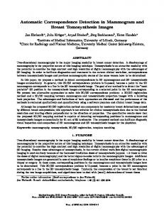
presentation of an Xflow classifier that seeks to separate avoidable from unavoidable Xflows and the F → Q type transformation on which it rests. We ran our experiments on a machine running Ubuntu 10.04.2 LTS (kernel 2.6.32-30-server) with 128GB RAM and 3 Intel Xeon X7542 6-Core 2.66GHz 18MB Cache, for a total of 18 cores. The Ariadne engine is described in Section 4. We choose to analyze the special functions of the GNU scientific library (GSL) version gsl1.14, because the first phase of Ariadne focuses on scalar functions and most of GSL’s special functions take and return scalars. We examined all the special functions in the GSL, even though some are static and others share their core implementation. The GSL is a mature, well-maintained, well-tested, widely deployed scientific library [15]. It is for these reasons that we selected it for analysis: finding nontrivial exceptions in it is both challenging and important. In spite of these challenges, Ariadne found nontrivial exceptions. Since Ariadne analyzes programs not functions, we applied a transformation to each special function in the GSL library that synthesizes a main that creates symbolic variables and calls the analyzed function, in addition to applying the transformations described in Section 3.2 and Section 4.1.

1000

100

10

1

Invalid

DivByZero

Overflow

Underflow

Figure 7: Ariadne found 2091 input-to-location pairs that trigger floating-point exceptions in the GNU Scientific library, distributed as shown. public API and the source of these 20 functions to 1) identify their preconditions and 2) check whether the exception-triggering inputs Z3-A RIADNE reported against these functions violated those preconditions. Two of the 20 functions were static; against these two functions, Z3-A RIADNE reports 7 input to exception pairs. Even though they had no explicit preconditions in their comments, their call sites may implicitly encode preconditions, so we conservatively deemed these 7 pairs to be false positives. Six functions had publicly documented preconditions. Against these 6 functions, Z3-A RIADNE reported 16 exception pairs, 2 of which violated the function’s precondition and are false positives. Against the remaining 12, Z3A RIADNE reported 64 input to exception pairs. In this experiment, 9 or 12%. therefore, Z3-A RIADNE’s false positive rate was 77 Path Injection For each operation, the Ariadne transformation doubles (quadruples in the case of division) the paths to the operation. The reason is that fabs uses a conditional to compute the absolute value of its operand. Consider “double pre = 1.0/sqrt(2.0*M_PI*x);”. Here, the expression passed to sqrt actually contains only one multiplication because the compiler replaces the constant multiplication 2.0*M_PI with a single constant. Considering only the multiplication in the operand of the sqrt, Ariadne injects the following pseudocode: 1 2 3 4 5

if ( x > 0 ) y = (2.0*M_PI*x) else y = -(2.0*M_PI*x) if (y > DBL_MAX) Overflow if (y < DBL_MIN) Underflow double pre = 1.0/sqrt(y);

In this example, Ariadne finds x = 2.861117e+307 that traverses 1, 3 and x = -2.861117e+307 that traverses 1, 2, 3; both inputs satisfy the conditional and trigger Overflow. 5.2

Analysis Performance and Results

Z3-A RIADNE found a total of 2091 input-to-location pairs that triggered exceptions, distributed as shown in Figure 7. Z3-A RIADNE finds many more Xflows than Invalid or Divide-by-Zero exceptions because programmers strive to avoid the latter and because Xflows can mask these exceptions, as when an underflow occurs in the evaluation of a denominator and terminates exploration of that path before the division is evaluated. Figure 8 shows the distribution of functions in terms of the potential exceptions they contain. As expected, this distribution is skewed: Given the maturity and popularity of the GSL, it is not surprising that most of its functions contain no latent floating-point exceptions. Ariadne reports the most exceptions, 152, in gsl_sf_bessel_Inu_scaled_asympx_e defined in gsl/specfunc/bessel.c: Perhaps the most serious exceptions are Divide-by-Zero and Invalid exceptions. For a selection of these exceptions, Table 3 and Ta-

Number of Functions (log scale)

1000

100

10

1 0

3

6

9 12 15 18 21 24 27 30 33 36 39 42 45 48 51 54 57 60

Number of Exception-triggering Input-to-Location Pairs

Figure 8: Bar plot of the number of functions (y-axis) with the specified number of input-to-location pairs that trigger floating-point exceptions (x-axis). Function (prefix gsl_sf_) conicalP_1_e bessel_Jnu_asympx_e exprel_n_CF_e bessel_Knu_scaled_asympx_e

Line

Inputs

989 234 89 317

2.0e+01, 1.0e+00 0.0, 0.0 -1.0e+00, 1.340781e+154 0.0, 0.0

Table 3: 4 of the 44 Divide-by-Zero exceptions Ariadne found. Function (prefix gsl_sf_bessel_) Inu_scaled_asymp_unif_e Knu_scaled_asympx_e Jnu_asympx_e Inu_scaled_asympx_e

Line

Inputs

361 317 234 302

-2.225074e-308, 0.0 -7.458341e-155, -8.654053e+01 -5.0e-01, 0.0 -1.5e+00, -3.921032e+03

Table 4: 4 of the 125 Invalid exceptions Ariadne found. ble 4 show the function in which we found this type of exception, the line number, and exception triggering inputs. For example, Ariadne found a Divide-by-Zero exception in gsl_sf_conicalP_1_e in gsl/specfunc/legendre_con.c. Line 989 of this file is “const

int stat_V = conicalP_1_V( th, x/sh, lambda, 1.0, &V0, &V1);”. When lambda = 20 and x = 1, sh = sqrt(x - 1.0) * sqrt(x + 1.0) = 0, so x/sh throws Divide-by-Zero, 122 lines

and 8 control points from function entry. Table 5 shows the results from our analysis of the scalar GSL special functions. The data shows that, over the GSL special functions, the loop bound (the first column) has little impact on the results. We believe that the reason for this is that the analyzed functions do not make heavy use of looping constructs. Z3-A RIADNE attempts to explore all paths within the per-run time bound it is given. When Z3-A RIADNE does not exhaust its per-run timeout when analyzing a function, we increment the “No Timeout” column. Z3-A RIADNE successfully explores a path when it determines that the path is satisfiable; when it finds an exception, that exception is real, i.e. it certainly occurs with the reported inputs, even though Z3-A RIADNE does not model rounding, because Z3-A RIADNE confirms candidate input-to-exception pairs via its concrete execution check (Section 3.3). Z3-A RIADNE’s abandonment of a path as unsatisfiable is provisional for the three reasons discussed in Section 3.3: it approximates floating-point semantics with reals, which notably ignores rounding; it concretizes multivariate into univariate constraints; and it bounds loops. Of these three, we can have some confidence when Z3-A RIADNE reports UNSAT due to concretization, because, as we describe above, concretization is effective due to the fact that the variables in our numerical constraints in practice either have few or many solutions. The former case causes Z3-A RIADNE to report unsatisfiable constraints. When reporting UNSAT, Z3-A RIADNE’s

precision is good, so the third column reports the count of functions Z3-A RIADNE fully explored without encountering a per-query timeout, i.e. U. In some of the functions it fully explored, Z3-A RIADNE discovered no exceptions; the count of these functions is in column four. The set of functions whose cardinality appears in the “No Timeout” column contains the “All Paths Explored” functions which contain the “No Exception Discovered” functions. We note that, while most of the functions in which Z3-A RIADNE discovered no exceptions at the infinity bound are loop-free, four are not. During Z3-A RIADNE’s analysis of the GSL, Z3 handled 48% of the total queries, while Ariadne handled the rest. Of the total queries made, we can guarantee the results for 76% at the infinity bound. The remaining 24% represent UNSAT results of which we cannot be certain, since they involve concretization. That said, our intensive concretization experiment shows that 92% of them are likely to be UNSAT, with 1M concretizations, we found 8% additional SAT. 24% · 8% = 1.9%, so Z3-A RIADNE is likely to incorrectly resolve around 2% of its constraints. The loop bound transformation monotonically reduces the number of paths in a program, so each of the function columns should be monotonically increasing. This pattern does not hold over “No Timeout” column. There are two reasons for this variation. First, Z3 randomly hangs on some of the nonlinear, multivariate constraints Z3-A RIADNE feeds it, in spite of its per-query timeout. Second, KLEE flips coins during path scheduling to ensure better coverage. In short, some of the analysis runs at certain loop bounds were simply unlucky. |S| The three columns that contain the ratios of SAT |Q| , UNSAT ¯ |S| |Q| ,

|U|

and UNKNOWN |Q| queries report on Z3-A RIADNE’s overall effectiveness. Recall that in Z3-A RIADNE, Ariadne only handles Z3’s unknown queries. The Ariadne ratio column reports Ariadne effectiveness at solving Z3’s unknowns in our context. Let SA , S¯A and UA be the SAT, UNSAT and UNKNOWN queries that Ariadne |S ∪S¯A | handles. The Ariadne ratio then is |S ∪AS¯ ∪U . In short, Ariadne A A A| found a substantial fraction of the exceptions and resolved 76–82% of the queries that Z3 was unable to handle. The “Unique” exception field shows [X,Y ], where X is the number of exception locations and Y is the number of unique input to exception location pairs found by Z3-A RIADNE only at the specified loop bound. In the case of the number of input to location pairs, only the pair is unique, not the path it take nor the exception it reaches. At loop bound 64, the unique exception field in Table 5 contains [3, 145]. This means that the analysis discovered 3 exceptions that it did not also find at another bound and 145 input to exception pairs, found only at this bound. The “Shared” also reports exceptions and paths to exceptions, but without the constraint that those exceptions and input to exception pairs were only discovered at the specified loop bound. Our analysis is embarrassingly parallelizable, so the test harness partitions the functions onto available cores (in our case 18), then analyzes each function, one by one, against each loop bound. It records the analysis time per function per loop bound. The sum of all the analysis times for all the functions at each loop bound is reported in the total time column. Again, we see that, with our corpus, the loop bound does not have much impact on analysis time. 5.3

Classifying Overflows and Underflows

Some overflows and underflows (Xflows) are an unavoidable consequence of finite precision. The addition Ω + Ω is a case in point. Some Xflows, however, may be avoided by changing the order of evaluation in or outright replacing the algorithm used to compute a solution. Because a developer’s time is precious, we introduce the avoidable Xflow classifier to distinguish potentially avoidable Xflows from those that are not.

Loop Bound

No Timeout

All Paths Explored

No Exception Discovered

|S| |Q|

¯ |S| |Q|

|U| |Q|

Ariadne Ratio

infinity 64 32 16 8 4 2 1

363 370 368 367 368 366 367 372

136 149 149 149 149 149 149 149

45 54 54 54 54 54 54 54

0.57 0.57 0.57 0.57 0.57 0.58 0.56 0.56

0.30 0.32 0.32 0.32 0.32 0.32 0.33 0.33

0.13 0.11 0.11 0.11 0.11 0.10 0.11 0.11

0.76 0.80 0.81 0.81 0.81 0.82 0.81 0.81

Exceptions Unique Shared [20,174] [3,145] [1,162] [0,142] [3,144] [0,138] [4,134] [4,144]

[636,847] [658,874] [651,859] [652,858] [652,862] [644,853] [644,863] [655,872]

Total Time (hours) 89 85 87 87 86 89 86 84

Table 5: The results of Z3-A RIADNE’s analysis of the 467 GSL special functions at the specified loop bounds. Here, Q is the set of all queries issued during analysis and S, S¯ and U partition Q into its SAT, UNSAT and UNKNOWN queries.

Avoidable? Total Ratio

Overflows

Underflows

98 155 0.63

180 217 0.83

Table 6: Potentially avoidable overflows and underflows. Let A : Fn → F be an algorithm implemented using floatingpoint and A be that same algorithm implemented using arbitrary precision arithmetic over Q. When A(~i) overflows or underflows, we deem that exception potentially avoidable if A (~i) falls within the range of normal floating-point numbers, i.e. |A (~i)| ∈ [λ , Ω]. This classifier rests on the intuition that, if the evaluation of a floating-point expression over arbitrary precision arithmetic falls within the range of normal floating-point numbers, then it may be possible to find an alternate expression that evaluates to that same result over floating-point without generating intermediate values that trigger floating-point exceptions. For example, consider Sterbenz’ y−x av3, where x+ 2 . When x = −Ω, y = Ω, the subtraction overflows under floating-point, but the final result is 0, a normal floating-point number. Further, we know that av1 is the algebraically equivalent (over the reals) expression x+y 2 that, in this case, generates the correct answer without intermediate overflow. To realize our Xflow classifier, we wrote a transformer that takes a numeric program and replaces its float and double types with an arbitrary precision rational type, for whose implementation we use mpq_t from GMP [14]. In addition to rewriting types, our arbitrary precision transformer also rewrites floating-point operations into rational operations. For instance, z = x + y becomes mpq_add(z,x,y). Xflows dominated the exceptions we found, comprising 91.9% of all exceptions. We defined and realized our classifier with the aim of filtering these Xflows. Nonetheless, the number of potentially avoidable Xflows remains high in Table 6. Note that GSL is a worst case for us. In a numerical library such as the GSL, these ratios are high because the range of many mathematical functions is small but their implementation relies on floating-point operations whose operands have extremal magnitude.

6.

Related Work

Ariadne is related to the large body of work on symbolic execution [27], such as recent representative work on KLEE [7] and DART [18]. Our work directly builds on KLEE and uses its standard symbolic exploration strategy. To the best of our knowledge, it is the first symbolic execution technique applied to the detection of floating-point runtime exceptions. We have proposed a novel programming transformation concept to reduce floating-point analysis

to reasoning on real arithmetic and developed practical techniques to solve nonlinear constraints. Our work is also closely related to the static analysis of numerical programs. The main difference of our work from these is our focus on bug detection rather than proving the absence of error — every exception we detect is a real exception, but we may miss some. We next briefly discuss representative efforts in this area. Majumdar et al. extended the Splat concolic testing engine to support floating-point and nonlinear constraints, then tackled the problems of path coverage, range and robustness analysis [30]. Lakhotia et al. empirically evaluated two search-based techniques for solving numerical constraints — alternating variable method and evolution strategies [28]. Their goal was to improve the solution of numerical constraints in general, not in our specific context of detecting floating-point exceptions. They found that these techniques do not decisively outperform Pex’ custom solvers. Godefroid and Kinder observed that numerical operations rarely appear in conditionals and therefore not in the path constraint [17]. They leverage this observation to build an analysis that aims to prove the memory safety of floating-point operations and the non-interference of the numeric and non-numeric parts of the subject program. This is in marked contrast with our work, where our transformation explicitly adds numeric conditions and solves the resulting constraints in order to detect floating-point exceptions. Goubault [20] developed an abstract interpretation-based static analysis [5] to analyze errors introduced by the approximation of floating-point arithmetic. Goubault and Putot later refined this work with a more precise abstract domain [21]. Brillout et al. encode floating-point operations as functions on bit vectors, then successively both over- and under-approximate the resulting formulae [2]. Martel [31] presents a general concrete semantics for floating-point operations to explain the propagation of roundoff errors in a computation. In later work [32], Martel applies this concrete semantics and designed a static analysis for checking the stability of loops [23]. Miné [34] proposes an abstract interpretation-based approach to detect floating point errors. Underflows and round-off errors are considered tolerable and thus not considered real run-time errors. Monniaux [35] summarizes the typical errors when using program analysis techniques to detect bugs in or verify correctness of numerical programs. Astree [6] statically analyzes C programs and attempts to prove the absence of overflows and other runtime errors, both over integers and floating-point numbers. Also related are different approaches to model the floating point computation for numerical programs. Fang et al. [11, 12] propose the use of affine arithmetic to model floating-point errors. Darulova et al. augment Scala with two new data types: AffineFloat, which computes error bounds while remaining compatible with the Double type and SmartFloat, which generalizes AffineFloat to sets of inputs [8]. Two projects that address floating-point accuracy

problems are Fluctuat [10] and a recent paper that dynamically shadows floating-point values and operations with higher precision operands and operators in order to detect accuracy loss, catastrophic cancellation in particular [1]. Ariadne complements these papers, since its focus is the detection of floating-point exceptions, not floating-point accuracy.

[13] M. Fränzle, C. Herde, T. Teige, S. Ratschan, and T. Schubert. Efficient solving of large non-linear arithmetic constraint systems with complex Boolean structure. JSAT, 1(3-4):209–236, 2007. [14] FSF. GMP: The GNU multiple precision arithmetic library. /http: //gmplib.org/. [15] FSF. GSL: GNU scientific library. http://www.gnu.org/s/ gsl/.

7.

[16] V. Ganesh and D. L. Dill. A decision procedure for bit-vectors and arrays. In CAV, 2007. [17] P. Godefroid and J. Kinder. Proving memory safety of floating-point computations by combining static and dynamic program analysis. In ISSTA, 2010. [18] P. Godefroid, N. Klarlund, and K. Sen. DART: Directed automated random testing. In PLDI, 2005.

Conclusion and Future Work

We have presented our design and implementation of Ariadne, a symbolic execution engine for detecting floating-point runtime exceptions. We have also reported our extensive evaluation of Ariadne over a few hundred GSL scalar functions. Our results show that Ariadne is practical, primarily enabled by our novel combination of program rewriting to expose floating-point exceptional conditions and techniques for nonlinear constraint solving. Our immediate future work is to publicly release the tool to benefit numerical software developers. We would also like to investigate approaches to support non-scalar functions, such as those functions that accept or return vectors or matrices.

8.

Acknowledgments

We thank Jian Zhang, Mark Gabel, David Hamilton, and the anonymous reviewers for constructive feedback on earlier drafts of this paper. We also thank Zhaojun Bai, William M. Kahan, and RenCang Li for helpful discussions on this work. This research was supported in part by NSF (grants 0702622, 0917392, and 1117603) and the US Air Force (grant FA9550-07-1-0532). The information presented here does not necessarily reflect the position or the policy of the government and no official endorsement should be inferred.

References [1] F. Benz, A. Hildebrandt, and S. Hack. A dynamic program analysis to find floating-point accuracy problems. In PLDI, 2012. [2] A. Brillout, D. Kroening, and T. Wahl. Mixed abstractions for floatingpoint arithmetic. In FMCAD, 2009. [3] CNN. Toyota: Software to blame for Prius brake problems. http://www.cnn.com/2010/WORLD/asiapcf/02/ 04/japan.prius.complaints/index.html. [4] P. Collingbourne, C. Cadar, and P. H. Kelly. Symbolic crosschecking of floating-point and SIMD code. In EuroSys, 2011. [5] P. Cousot and R. Cousot. Abstract interpretation: A unified lattice model for static analysis of programs by construction or approximation of fixpoints. In POPL, 1977. [6] P. Cousot, R. Cousot, J. Feret, L. Mauborgne, A. Miné, D. Monniaux, and X. Rival. The ASTRÉE analyzer. In ESOP, 2005. [7] D. E. Daniel Dunbar, Cristian Cadar. KLEE: Unassisted and automatic generation of high-coverage tests for complex systems programs. In OSDI, 2008. [8] E. Darulova and V. Kuncak. Trustworthy numerical computation in Scala. In OOPSLA, 2011. [9] L. De Moura and N. Bjørner. Z3: An efficient SMT solver. In TACAS, 2008. [10] D. Delmas, E. Goubault, S. Putot, J. Souyris, K. Tekkal, and F. Védrine. Towards an industrial use of FLUCTUAT on safety-critical avionics software. In FMICS, 2009. [11] C. F. Fang, T. Chen, and R. A. Rutenbar. Floating-point error analysis based on affine arithmetic. In ICASSP, 2003. [12] C. F. Fang, R. A. Rutenbar, M. Püschel, and T. Chen. Toward efficient static analysis of finite-precision effects in DSP applications via affine arithmetic modeling. In DAC, 2003.

[19] D. Goldberg. What every computer scientist should know about floating-point arithmetic. ACM Computing Surveys, 23(1), 1991. [20] E. Goubault. Static analyses of the precision of floating-point operations. In SAS, 2001. [21] E. Goubault and S. Putot. Static analysis of numerical algorithms. In SAS, 2006. [22] J. Hauser. Handling floating-point exceptions in numeric programs. TOPLAS, 18(2), 1996. [23] N. J. Higham. Accuracy and stability of numerical algorithms. Society for Industrial and Applied Mathematics, 2nd edition, 2002. [24] IEEE Computer Society. IEEE standard for floating-point arithmetic, 2008. [25] D. Jovanovi´c and L. de Moura. Solving non-linear arithmetic. In IJCAR, 2012. [26] W. Kahan. A demonstration of presubstitution for ∞/∞ (Grail), 2005. [27] J. C. King. Symbolic execution and program testing. Communications of the ACM, 19, 1976. [28] K. Lakhotia, N. Tillmann, M. Harman, and J. De Halleux. FloPSy: search-based floating point constraint solving for symbolic execution. In ICTSS, 2010. [29] C. Lattner and V. Adve. LLVM: A compilation framework for lifelong program analysis & transformation. In CGO, 2004. [30] R. Majumdar, I. Saha, and Z. Wang. Systematic testing for control applications. In MEMOCODE, 2010. [31] M. Martel. Propagation of roundoff errors in finite precision computations: a semantics approach. In ESOP, 2002. [32] M. Martel. Static analysis of the numerical stability of loops. In SAS, 2002. [33] Z. Merali. Computational science: ...error ...why scientific programming does not compute. Nature, 467:775–777, 2010. [34] A. Miné. Relational abstract domains for the detection of floating-point run-time errors. In ESOP, 2004. [35] D. Monniaux. The pitfalls of verifying floating-point computations. TOPLAS, 30(3):12:1–12:41, 2008. [36] K. L. Palmerius. Fast and high precision volume haptics. In Proceedings of the IEEE World Haptics Conference. IEEE, 2007. [37] P. Rümmer and T. Wahl. An SMT-LIB theory of binary floating-point arithmetic. In SMT at FLoC, 2010. [38] K. Sen. CUTE: a concolic unit testing engine for C. In FSE, 2005. [39] P. H. Sterbenz. Floating-Point Computation. Prentice-Hall, 1974. [40] Wikipedia. Ariane 5 flight 501. http://en.wikipedia.org/ wiki/Ariane_5_Flight_501.