Neural Networks and achieved an accuracy of 91.6% when using MFCC, with an improvement to 92.3% when adding pitch and energy. Adding video features ...
Automatic Detection of Laughter and Fillers in Spontaneous Mobile Phone Conversations Hugues Salamin∗ , Anna Polychroniou∗ and Alessandro Vinciarelli∗† ∗ University
of Glasgow - School of computing Science, G128QQ Glasgow, UK Research Institute - CP592, 1920 Martigny, Switzerland {hsalamin,annap,vincia}@dcs.gla.ac.uk
† Idiap
Abstract—This article presents experiments on automatic detection of laughter and fillers, two of the most important nonverbal behavioral cues observed in spoken conversations. The proposed approach is fully automatic and segments audio recordings captured with mobile phones into four types of interval: laughter, filler, speech and silence. The segmentation methods rely not only on probabilistic sequential models (in particular Hidden Markov Models), but also on Statistical Language Models aimed at estimating the a-priori probability of observing a given sequence of the four classes above. The experiments are speaker independent and performed over a total of 8 hours and 25 minutes of data (120 people in total). The results show that F1 scores up to 0.64 for laughter and 0.58 for fillers can be achieved. Index Terms—Laughter Detection, Fillers Detection, Nonverbal Vocal Behavior, Hidden Markov Model, Statistical Language Models.
I. I NTRODUCTION The computing community dedicates significant efforts to the development of socially intelligent technologies, i.e. automatic approaches capable of sensing the social landscape in the same way as people do in their everyday life [1], [2]. In this context, the detection of nonverbal behavior (facial expressions, vocalisations, gestures, postures, etc.) plays a fundamental role because nonverbal cues are one of the main channels through which we convey social signals, namely “acts or structures that influence the behavior or internal state of other individuals” [3], “communicative or informative signals which [...] provide information about social facts” [4], or “actions whose function is to bring about some reaction or to engage in some process” [5]. In particular, this article considers the automatic detection of laughter and fillers, widely recognized as two of the most important social signals that can be observed in social interactions. This applies in particular to mobile phone calls, the setting adopted for the experiments of this work, where people cannot see one another and, therefore, vocal cues are the only form of nonverbal behavior that can be adopted. Laughter [6] corresponds to vocal outbursts typical of amusement, joy, scorn or embarrassment . Fillers [7] are vocalisations like “uhm”, “eh”, “ah” etc. “filling” the time that should be occupied by a word (generally in correspondence of hesitations, uncertainty or attempts to hold the floor). The experiments are performed over the SSPNet Vocalization Corpus, a collection of 2763 audio clips each including at least one laughter or filler instance (see Section III for more details). To the best of our knowledge, this is one of the largest
databases of this type in terms of both amount of instances (2988 for laughter and 1158 for fillers) and number of subjects (120 in total). Besides improving the statistical reliability of the results, this allowed us to reinforce the state-of-the-art (see Section II for a short survey) under several respects. The first is the development of speaker independent approaches, i.e. statistical models trained over individuals different from those used for the tests. In several works of the literature, this was not possible because the available material was not sufficient to separate the speakers. The second is that our approach is not only fully automatic (manual segmentation into speech and non-speech is not required as in other works), but also addresses jointly the detection of laughter, fillers, speech and silence, tasks that are typically separated in other works of the literature. This makes it possible to introduce the third important aspect of this work, namely the adoption of Statistical Language Models aimed at estimating the a-priori probability of observing a given sequence of the four classes above. To the best of our knowledge, this was not done before for detecting vocal cues. The rest of the article is organized as follows: Section II surveys the main works dedicated to laughter and fillers detection, Section III presents the SSPNet Vocalization Corpus adopted for the experiments, Section IV describes the detection approach, Section V reports on experiments and results, and the final Section VI draws some conclusions. II. S TATE - OF - THE -A RT To the best of our knowledge, no major efforts were done to detect fillers while laughter was the subject of several works. Therefore, most of the works presented in this section focus on laughter detection. Two main problems were addressed in the literature. The first, called classification hereafter, is performed over collections of audio samples (typically around one second of length) that include either laughter or other forms of vocal behavior (speech, silence, etc.). The classification problem consists in correctly discriminating between laughter samples and the others. The second problem, called segmentation hereafter, consists in automatically splitting audio recordings into intervals corresponding either to laughter or to other observable behaviors (overlapping speech, hesitations, etc.). The rest of this section surveys the main works dedicated to both problems (see Table I for a synopsis).
TABLE I T HE TABLE REPORTS THE DETAILS OF THE MAIN RECENT WORKS ON LAUGHTER DETECTION PRESENTED IN THE LITERATURE . T HE FOLLOWING ABBREVIATIONS ARE USED : A=AUDIO , V=V IDEO , C=C LASSIFICATION , S=S EGMENTATION , ACC =ACCURACY, EER=E QUAL E RROR R ATE ,
Ref.
Dataset
Instances
Modality
Task
[8]
ICSI Meetings, 29 meetings, 25 h, 16 subjects
1926 laughter events
A
C
EER 13%
[9]
ICSI and CGN, 3 h 38’, 24 subjects, 2 languages
3574 (53.3%)
A
C
Acc. 64.0% (different Language) to 97.0% (same speakers)
[10]
7 AMI meetings & SAL Dataset, 16’, 25 subjects
218 Laughter, Non-Laughter
AV
C
Acc. 85.4% − 92.3% for A. Acc. 94.7% for combination with V
[11]
AVIC, 21 subjects, 2291 clips
261 Laughter
A
C
5 classes: Breathing, Consent, Garbage, Hesitation, Laughter. Acc 77.8% − 80.7%
[12]
ICSI Meetings, 29 meetings, 25 h, 16 subjects
1h33’ of (6.2% )
laughter
A
S
F1 ∼ 0.62
[13], [14]
ICSI Meetings, 29 meetings, 25 h, 16 subjects
1h33’ of (6.2% )
laughter
A
S
Silence manually removed, F1 0.81
[15], [16]
ICSI Meetings, 29 meetings, 25 h, 16 subjects
16.6’ of laughter (2.0% of test set)
A
S
Automatic detection of silence. F1 0.35 on voiced laughter, 0.44 on unvoiced laughter.
[17], [18]
FreeTalk Data, 3h, 4 subjects
10% is Laughter
AV
S
F1 0.44 − 0.72. Any laughter segment partially labelled is counted as fully detected for the computation of recall in F1 .
Laughter 331
A. The Classification Problem Classification is the most popular task for automatic laughter detection and was first investigated in [8]. The initial data consisted of 29 meetings with 8 participants recorded using tabletop microphones. Clips of one second length were then extracted and labelled as “laughter” or “non-laughter” based on the number of participants laughing at the same time. Therefore, the approach detected only events where several participants were laughing. Thee experiments were performed over a corpus of clips including 1926 laughter samples. The samples were represented with Mel-Frequency Cepstral Coefficients (MFCC) and Modulation Spectrum features. The classification was performed with Support Vector Machines (SVM) and the best Equal Error Rate, achieved with MFFC only, was 13%. In [9], the experiments were performed over 6838 clips for a total of 3 hours and 38 minutes extracted from meeting recordings. The training set was composed of 5102 clips in English and three test sets where used in order to compare different conditions (same speakers as in training set, different speakers, different languages). Four types of features were investigated: Perceptual Linear Prediction Coding features (PLP), Pitch and Energy (on a frame by frame basis), Pitch and Voicing (at the clips level) and Modulation Spectrum features. The classification was performed with Gaussian Mixture Models (GMM), SVMs and Multi Layer Perceptrons. The main finding was that PLP features used with GMM produce the highest accuracy (82.4% to 93.6%). When combining the output of several classifiers on different features, the accuracy can be improved up to 97.1% (by combining GMM trained on PLP and SVM trained on pitch and voicing features at the utterance level). In [10], the authors investigate the joint use of audio (MFCC, and pitch and energy based statistics) and video
Performance
features (head pose and facial expressions are extracted by tracking landmarks on the face of people) for laughter detection. The dataset is composed of 649 clips (218 laughter events) extracted from meeting recordings and from interactions between humans and artificial agents. The classifiers were Neural Networks and achieved an accuracy of 91.6% when using MFCC, with an improvement to 92.3% when adding pitch and energy. Adding video features brings the accuracy to 94.7%. The only work on classification of laughter versus other types of non-verbal vocalization we are aware of is in [11]. The data is composed of 2901 clips divided in 5 classes: Breathing, Consent, Garbage, Hesitation and Laughter. The authors investigate three models: Hidden Markov Models, Hidden Conditional Random Fields (hCRF) and SVM. The performances of the three models using MFCC and PLP features were compared. The best performance was achieved with HMMs and PLP features (80.7% accuracy). B. The Segmentation Problem The segmentation problem is addressed in this article as well and, on average, it is more challenging than the classification one. In segmentation, the input is not split a-priori into laughter and non-laughter and the goal is to identify laughter segments in the data stream. In [12], the authors extended the work in [9] and assessed their approach on a segmentation task. The proposed approach adopted PLP features to train Hidden Markov Models with GMM as emission probability distributions. The data set consisted of 29 meetings, with 3 meetings held out as a test set. The Markov model achieved an F1 score of 0.62 for the segmentation of laughter versus the rest. The work in [13], [14] investigates the use of Multi-Layer Perceptrons for the segmentation of laughter in meetings. The approach used MFCC features, Pitch and Energy. An
HMM model fitted on the output of the MLP to take into account the temporal dynamics and a F1 score of 0.81 was achieved. However, the approach was tested only with the silence segments manually removed. Furthermore, segments were the subjects were laughing and speaking at the same time were manually removed. In [16], [15], the authors presented a system for segmenting the audio of meetings in three classes: silence, speech and laughter. Their approach is based on HMMs and uses MFCC and energy as features. The approach takes into account the state of all the participants when segmenting a meeting and achieves a F1 score of 0.35 for laughter. In [18], audio-visual data from 2 meetings involving 4 speakers were segmented into laughter and non-laughter. Modulation Spectrum and PLP features were extracted from the audio. The features extracted from the video did not provide any improvement when used in combination with the audio features. The authors used 3 models: HMM, GMM and Echo State Networks, with the HMM outperforming the other two models with a F1 score of 0.72. However, the recall was computed by considering fully detected also laughter events that were automatically detected only partially. This leads to an overestimate of recall and F1 score. III. T HE SSPN ET VOCALIZATION C ORPUS The SSPNet Vocalisation Corpus (SVC) includes 2763 audio clips (11 seconds long each) annotated in terms of laughter and fillers for a total duration of 8 hours and 25 minutes. The corpus was extracted from a collection of 60 phone calls involving 120 subjects [19], 63 women and 57 men. The participants of each call were fully unacquainted and never met face-to-face before or during the experiment. The calls revolved around the Winter Survival Task: the two participants had to identify objects (out of a predefined list) that increase the chances of survival in a polar environment . The subjects were not given instructions on how to conduct the conversation, the only constraint was to discuss only one object at a time. The conversations were recorded on both phones (model Nokia N900) used during the call. The clips were recorded with the microphones of the phones. Therefore they contain the voice of one speaker only. Each clip lasts for 11 seconds and was selected in such a way that it contains at least one laughter or filler event between t = 1.5 seconds and t = 9.5 seconds. Clips from the same speaker never overlap. In contrast, clips from two subjects participating in the same call may overlap (for example in the case of simultaneous laughter). However, they do not contain the same audio data because they are recorded with different phones. Overall, the database contains 1158 filler instances and 2988 laughter events. Both types of vocalisation can be considered fully spontaneous. IV. T HE A PPROACH The experiments aim at segmenting the clips of the SVC into laughter, filler, silence and speech. More formally, given a sequence of acoustic observations X = x1 , . . . , xn , extracted
at regular time steps from a clip, we want to find a segmentation Y = (y1 , s1 ), . . . , (ym , sm ), with yi ∈ {f, l, p, s}1 , si ∈ {1, . . . , n}, s1 = 0 and si < si+1 . This encodes the sequence of labels and when they start. We set sm+1 = n to ensure that the segmentation covers the whole sequence. We will use a maximum a-posteriori approach to find the following sequence Yˆ of labels: Yˆ = arg max P(X, Y ), Y ∈Y
(1)
where Y is the set of all possible label sequences of length between 1 and n. The rest of the section is organized in two parts. The first describes the model we use for estimating P(X, Y ). The second describes the speech features extracted and the different parameters that need to be set in the model. A. Hidden Markov Model A full description of Hidden Markov Models is available in [20]. HMMs can be used to model a sequence of real valued vector observations X = x1 , . . . , xn with xi ∈ Rm . The model assumes the existence of latent variables H = h1 , . . . , hn and defines a joint probability distribution over both latent variables and observations: n Y P(X, H) = P(x1 | h1 )·P(h1 )· P(xi | hi )·P(hi | hi−1 ). (2) i=2
From this joint distribution, the probability of the observations can be computed by marginalizing the latent variables: X P(X) = P(X, H). (3) H∈H
H is the set of all possible sequences of latent variables of length n. The sum can be efficiently computed using Viterbi decoding even thought the size of H make direct summation intractable. We train a different HMM Py (X, H) for each label y ∈ {f, l, p, s} using sequences of observations extracted from the clips of the training set. The four HMMs, called acoustic models hereafter, capture the acoustic characteristics of the four classes corresponding to the labels. The probability of the whole sequence is given by P(X, Y ) = P(Y ) ·
m Y
Pyi (Xsi ···si+1 ),
(4)
i=1
where Xsi ···si+1 = xsi , . . . , xsi+1 , and Pyi corresponds to the probability given by the HMM model trained on sequences associated with the label yi . In previous works, P(Y ), usually called the language model, was assumed to be uniform and was therefore ignored. In this work, P(Y ) is modeled explicitly: !λ m m Y Y P(X, Y ) = Pyi (Xsi ···si+1 ) P(yi | yi−1 ) , (5) i=1
i=2
where P(yi | yi−1 ) corresponds to a bigram language model. The parameter λ is used to adjust the relative importance of 1 labels
are (f)iller, (l)aughter, s(p)eech, (s)ilence
the language model with respect to the acoustic model. When λ 6= 1 in Equation (5), P(X, Y ) is not normalized. However, this does not represent a problem because the segmentation process aims at finding the label sequence Yˆ maximizing the probability and not its exact value, as shown in Equation (1).
Filler
1.0 0.9 0.8
B. Features and Model Parameters The experiments were conducted using the HTK Toolkit [21] for both extracting the features and training the Hidden Markov Models (HMM) used for the segmentation. The parameters for the feature extraction were set based on the current state-of-the-art. For each clip, MFCC were extracted every 10 ms, from a 25 ms long Hamming window. We extracted 13 MFCC using a Mel filter bank of 26 channels. The log-energy of every windows was used instead of the zeroth coefficient. The feature vectors were extended using first and second order regression coefficients. The resulting feature vectors have dimension 39. For the HMM, we used a left-right topology. Four acoustic models were trained, one for each of the four classes (silence, speech, laughter and fillers). Each model has 9 hidden states and each hidden state uses a mixture of 8 Gaussian distributions with diagonal covariance matrix. This topology has been shown to work well in practice. Furthermore, it enforces a minimum duration of 90 ms for each segment. The language model is a back-off bigram model, with Good-Turing discounting.
0.7 0.6 0.5 0.4
0
50
100
150
200
150
200
150
200
Laughter
1.0 0.9 0.8 0.7 0.6 0.5 0.4
0
50
100
Speech
1.0
V. E XPERIMENTS AND R ESULTS We adopted two experimental protocols. In the first, the clips in the corpus were split into five folds in order to conduct cross-validation. The folds were created such that each speaker is guaranteed to appear only in one fold and such that the folds are of approximately the same size (between 547 and 555 clips). Each fold was used, iteratively, as a test set while the others were used as training set. In the second protocol, the corpus was divided into two parts, using the clips of 60 speakers as training set and the clips of the other 60 speakers as test set. Both setups guarantee that no speaker appears in both test and training set. Therefore, all performances reported in Section V-A are speaker independent. The first protocol aims at using the entire corpus as test set while maintaining a rigorous separation between training and test data. The second protocol corresponds to the experimental setup of the Computational Paralinguistics Challenge2 (to be held at Interspeech 2013). This will allow one to compare the results of this work with those obtained by the challenge participants. A. Performance Measures One of the main challenges of the experiments is that the classes are heavily unbalanced. In the SVC, laughter accounts for slightly less than 3.5% of the time, fillers account for 5.0%, silence represents 40.2% and speech is 51.3% of the total time. Given this distribution, accuracy (the percentage of time frames correctly labelled) is not a suitable performance 2 emotion-research.net/sigs/speech-sig/is13-compare
0.9 0.8 0.7 0.6 0.5 0.4
0
50
100
Silence
1.0 0.9 0.8 0.7 0.6
F1 score
0.5
Precision π Recall ρ
0.4
0
50 100 150 Language Model weight λ
200
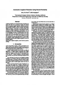
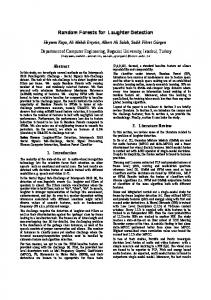
Fig. 1. The plots show how F1 Score, Precision and Recall change as a function of the parameter λ, the weight adopted for the Language Model. The plots have been obtained for the five-fold protocol, but the Figures for the other setup show similar behaviors.
TABLE II HMM PERFORMANCE OVER THE 5- FOLD SETUP. Precision π
F1 Score λ
Recall ρ
0
1
10
50
100
0
1
10
50
100
0
1
10
50
100
Filler
0.49
0.51
0.54
0.58
0.57
0.35
0.37
0.40
0.48
0.51
0.82
0.82
0.81
0.74
0.65
Laughter
0.48
0.53
0.58
0.64
0.63
0.35
0.39
0.45
0.60
0.67
0.79
0.80
0.79
0.69
0.61
Speech
0.77
0.79
0.81
0.83
0.84
0.94
0.95
0.94
0.91
0.89
0.65
0.67
0.70
0.76
0.79
Silence
0.87
0.88
0.87
0.87
0.86
0.82
0.82
0.82
0.82
0.82
0.92
0.93
0.93
0.92
0.91
TABLE III HMM PERFORMANCE OVER THE CHALLENGE SETUP. Precision π
F1 Score λ
Recall ρ
0
1
10
50
100
0
1
10
50
100
0
1
10
50
100
Filler
0.50
0.52
0.54
0.59
0.58
0.36
0.39
0.40
0.49
0.64
0.80
0.76
0.79
0.73
0.64
Laughter
0.49
0.54
0.59
0.65
0.63
0.37
0.42
0.49
0.65
0.56
0.74
0.76
0.74
0.66
0.56
Speech
0.77
0.79
0.80
0.83
0.84
0.94
0.94
0.94
0.91
0.80
0.66
0.68
0.70
0.76
0.80
Silence
0.85
0.86
0.86
0.85
0.85
0.80
0.80
0.80
0.80
0.91
0.91
0.93
0.93
0.91
0.91
measure. Therefore, for each class, we use precision π, recall ρ and F1 Score. For a given class y, we consider as positive all frames in the time intervals labelled as y and as negative frames those of all other intervals. Then, we define true positive frames (TP) every correctly classified positive frame and false positive frames (FP) every positive frame incorrectly classified. Similarly we can define true negative frames (TN) and false negative frames (FN). We can now define π as follows: TP , (6) TP + FN the fraction of samples labelled with a given class that actually belong to such a class. We also define ρ: π=
TP , (7) TP + FP the fraction of samples from the class of interest that are correctly classified. The F1 Score is a single score that takes into account both precision and recall and is defined as follows: π·ρ F1 = 2 · . (8) π+ρ ρ=
In the rest of this section, when testing if the difference between two models is statistically significant, we will use the Kolmogorov-Smirnov test (KS test) to compare the distribution of F1 Score over the audio clips. B. Detection Results Tables II and III present the results for the segmentation task using different values of λ, for both experimental protocols described above. Figure 1 shows how π, ρ and F1 Score change when λ ranges between 1 and 200 to provide a full account of the effect of such a parameter. For low values of λ, the Language Model does not influence the segmentation process and the performances are close to those obtained when using only the HMMs. The reason is that the contribution of the HMM term in Equation (5) tends to dominate with respect to the Language Model term. Hence, the
value of λ must be increased to observe the actual effect of the bigrams. In fact, when λ = 10, 50, 100, the F1 Score shows a significant improvement with respect to the application of the HMMs only. Since the goal of the experiments presented here is to show that the Language Model carries information useful for the segmentation process, no cross-validation is performed to set the λ value leading to the highest F1 Score. The results are rather reported for several λ values. When λ is too high, the F1 Score tends to drop for laughter and fillers (see Figure 1). The reason is that the Language Model tends to favour the most frequent classes (in this case speech). Hence, when λ is such that the Language Model becomes the dominant term of Equation (5), the segmentation process tends to miss laughter events and fillers. This phenomenon appears clearly when considering the effect of λ on Precision and Recall for the various classes. For laughter and fillers, π tends to increase with λ while ρ tends to decrease. In the case of speech, the effect is inverted, while for silence no major changes are observed (see Figure 1). An interesting insight in the working of the model is given by the confusion matrix in Table IV. The Table applies to the case λ = 100, but different weights lead to similar matrices. Most of the confusions occur between fillers and speech, as well as between laughter and speech. This is due to the fact that sometimes people speak and laugh at the same time, but the corresponding frames were still labeled as laughter. Similarly, fillers and speech both include the emission of voice and are acoustically similar. The confusion between silence and laughter is also significant. This is due to the presence of unvoiced laughter, for which acoustic characteristics are close to silence (absence of voice emission, low energy). VI. C ONCLUSIONS This work has proposed experiments on automatic detection of laughter and fillers in spontaneous phone conversations. The results were performed over the SSPNet Vocalization Corpus, one of the largest datasets available in the literature in terms
TABLE IV C ONFUSION M ATRIX FOR THE 2- GRAM GRAMMAR WITH λ = 100. T HE LINE CORRESPOND TO THE GROUND TRUTH AND THE COLUMN TO THE CLASS ATTRIBUTED BY THE CLASSIFIER . E ACH CELL IS A TIME IN SECONDS
filler
laughter
silence
voice
989
8
79
440
laughter
7
601
144
311
silence
83
105
11182
825
voice
584
120
1883
12949
filler
of both number of subjects and amount of laughter events and fillers (see Section III). To the best of our knowledge, this is the first attempt to jointly segment spontaneous conversations into laughter, fillers, speech and silence. Such a task can be considered more challenging than the simple classification of audio samples (see Section II) or the application of segmentation processes to audio manually presegmented into silence and speech. The most important innovation of the work is the adoption of Statistical Language Models aimed at estimating the a-priori probability of segment sequences in the data like, e.g., the probability of laughing after a silence and before speaking. The results show that the Language Models can significantly improve the performance of purely acoustic models. However, it is necessary to find an appropriate trade-off (by setting the parameter λ) between the weight of the HMMs and the weight of the bigrams. The results of this work can be considered preliminary and futher work is needed to achieve higher performances. In particular, the current version of the approach does not discriminate between voiced and unvoiced laughter, a distinction that has been shown to be effective in several works. Furthermore, the acoustic features are basic - although they have been shown to be effective in the literature - and can certainly be improved to capture subtle differences between, e.g., speech and fillers or silence and unvoiced laughter. ACKNOWLEDGMENTS The research that has led to this work has been supported in part by the European Community’s Seventh Framework Programme (FP7/2007-2013), under grant agreement no. 231287 (SSPNet), and in part by the Swiss National Science Foundation via the National Centre of Competence in Research IM2 (Information Multimodal Information Management). R EFERENCES [1] A. Vinciarelli, M. Pantic, and H. Bourlard, “Social Signal Processing: Survey of an emerging domain,” Image and Vision Computing Journal, vol. 27, no. 12, pp. 1743–1759, 2009. [2] A. Vinciarelli, M. Pantic, D. Heylen, C. Pelachaud, I. Poggi, F. D’Errico, and M. Schroeder, “Bridging the Gap Between Social Animal and Unsocial Machine: A Survey of Social Signal Processing,” IEEE Transactions on Affective Computing, vol. 3, no. 1, pp. 69–87, 2012. [3] M. Mehu and K. Scherer, “A psycho-ethological approach to social signal processing,” Cognitive Processing, vol. 13, no. 2, pp. 397–414, 2012.
[4] I. Poggi and F. D’Errico, “Social Signals: a framework in terms of goals and beliefs,” Cognitive Processing, vol. 13, no. 2, pp. 427–445, 2012. [5] P. Brunet and R. Cowie, “Towards a conceptual framework of research on social signal processing,” Journal of Multimodal User Interfaces, vol. 6, no. 3-4, pp. 101–115, 2012. [6] J. Vettin and D. Todt, “Laughter in Conversation: Features of Occurrence and Acoustic Structure,” Journal of Nonverbal Behavior, vol. 28, no. 2, pp. 93–115, Jan. 2004. [7] H. Clark and J. Fox Tree, “Using¡ i¿ uh¡/i¿ and¡ i¿ um¡/i¿ in spontaneous speaking,” Cognition, vol. 84, no. 1, pp. 73–111, 2002. [8] L. S. Kennedy and D. P. Ellis, “Laughter detection in meetings,” in NIST ICASSP 2004 Meeting Recognition Workshop, Montreal. National Institute of Standards and Technology, 2004, pp. 118–121. [9] K. P. Truong and D. A. Van Leeuwen, “Automatic discrimination between laughter and speech,” Speech Communication, vol. 49, no. 2, pp. 144–158, 2007. [10] S. Petridis and M. Pantic, “Audiovisual discrimination between speech and laughter: why and when visual information might help,” Multimedia, IEEE Transactions on, vol. 13, no. 2, pp. 216–234, 2011. [11] B. Schuller, F. Eyben, and G. Rigoll, “Static and dynamic modelling for the recognition of non-verbal vocalisations in conversational speech,” in Perception in multimodal dialogue systems. Springer, 2008, pp. 99–110. [12] K. Truong and D. van Leeuwen, “Evaluating automatic laughter segmentation in meetings using acoustic and acoustics-phonetic features,” in Proc. ICPhS Workshop on The Phonetics of Laughter, Saarbr¨ucken, Germany, 2007, pp. 49–53. [13] M. Knox and N. Mirghafori, “Automatic laughter detection using neural networks,” in Proceedings of interspeech, 2007, pp. 2973–2976. [14] M. Knox, N. Morgan, and N. Mirghafori, “Getting the last laugh: Automatic laughter segmentation in meetings,” in Proc. INTERSPEECH, 2008, pp. 797–800. [15] K. Laskowski, “Contrasting emotion-bearing laughter types in multiparticipant vocal activity detection for meetings,” in Acoustics, Speech and Signal Processing, 2009. ICASSP 2009. IEEE International Conference on. IEEE, 2009, pp. 4765–4768. [16] K. Laskowski and T. Schultz, “Detection of laughter-in-interaction in multichannel close-talk microphone recordings of meetings,” in Machine Learning for Multimodal Interaction. Springer, 2008, pp. 149–160. [17] S. Scherer, F. Schwenker, N. Campbell, and G. Palm, “Multimodal laughter detection in natural discourses,” in Human Centered Robot Systems. Springer, 2009, pp. 111–120. [18] S. Scherer, M. Glodek, F. Schwenker, N. Campbell, and G. Palm, “Spotting laughter in natural multiparty conversations: A comparison of automatic online and offline approaches using audiovisual data,” ACM Transactions on Interactive Intelligent Systems (TiiS), vol. 2, no. 1, p. 4, 2012. [19] A. Vinciarelli, H. Salamin, A. Polychroniou, G. Mohammadi, and A. Origlia, “From nonverbal cues to perception: Personality and social attractiveness,” Cognitive Behavioural Systems, pp. 60–72, 2012. [20] L. Rabiner and B. Juang, “An introduction to hidden markov models,” ASSP Magazine, IEEE, vol. 3, no. 1, pp. 4–16, 1986. [21] S. Young, G. Evermann, M. Gales, T. Hain, D. Kershaw, X. Liu, G. Moore, J. Odell, D. Ollason, D. Povey et al., “The htk book,” Cambridge University Engineering Department, vol. 3, 2002.