Ant Colony System for Segmentation and Classification of Microcalcification in Mammograms K.Thangavel1, M.Karnan2*, R.Sivakumar3, A. Kaja Mohideen3 1: Department of Mathematics, Gandhigram Rural Institute-Deemed University, 2: Department of computer science, Gandhigram Rural Institute-Deemed University, Gandhigram-624302, Tamil Nadu, India. Email:
[email protected] 3: Department of Computer Science and Engineering, R.V.S.College of Engineering & Technology, Dindigul, Tamil Nadu, India.
Abstract Detection of microcalcification based on textural image segmentation and classification is the most effective early-diagnosis of breast cancer. In this paper, a proposed technique, Markov Random Field method hybrid with Ant Colony System, Genetic Algorithm and Backpropagation Network (MRF–ACSGA-BPN) is implemented for the detection of microcalcification in digital mammogram. Identification of microcalcification is performed in two steps namely, segmentation and classification. First, the mammogram image is segmented using MRF-ACSGA method to extract the suspicious region. Second, the conventional textural analysis methods such as Spatial Gray Level Dependency Method (SGLDM), Surrounding Region Dependence Method (SRDM), Gray-Level Run-Length Method (GLRLM) and Gray Level Difference Method (GLDM) are used to extract the features from the segmented image. A three-layer Backpropagation Neural Network classifier, trained by jack knife method and round robin method, is used to classify the extracted features into benign or malignant. The classification performances for the texture-analysis methods are evaluated using a Receiver OperatingCharacteristics (ROC) analysis. The proposed algorithm and the techniques are tested on 161 pairs of digitized mammograms from MIAS database. Keywords: Mammogram, Markov Random Field, Ant Colony Optimization, Genetic Algorithm, Backpropagation Neural Network.
1
Introduction
Breast cancer is one of the major causes for the increase in mortality among women, especially in developed and under developed countries. The World Health Organization’s International agency for Research on Cancer in Lyon, France, estimates that more than 150 000 women worldwide die of breast cancer each year. The breast cancer is one among the top three cancers in American women. In the United States, the American Cancer Society estimates that, 215 990 new cases of breast carcinoma has been diagnosed, in 2004. It is the leading cause of death due to cancer in women under the age of 65. In India, breast cancer accounts for 23% of all the female cancers followed by cervical cancers (17.5%) in metropolitan cities such as Mumbai, Calcutta, and Bangalore. However, cervical cancer is still number one in rural India. Although the incidence is lower in India than in the developed countries, the burden of breast cancer in India is alarming [7]. Organ chlorines are considered a possible cause for hormonedependent cancers [47]. Detection of early and subtle signs of breast cancer requires high-quality images and skilled mammographic interpretation [54]. Although computer-aided mammography has been studied over the last two decades, automated interpretation of microcalcifications still remains very difficult. The dense tissues, and especially in younger women, cause suspicious region to be almost invisible and may be easily misinterpreted
as calcifications and yield a high False Positive (FP) rate that is a major problem with most of the existing algorithms. Double readings, as carried out, for example, by two radiologists, usually improve the quality of diagnostic findings, thus, greatly reducing the probability of misdiagnosis. On these grounds, adequate computational tools are expected to be helpful to the radiologist. Thangavel et al., [51] presented a study on methods of various stages on automatic detection of microcalcification in digital mammograms. According to those studies it is noted that the Ant Colony Optimization (ACO) has not been implemented in the field of mammogram analysis. In this paper, meta-heuristic algorithms such as GA and ACO are implemented to extract the suspicious region. The textural features can be extracted from the suspicious region to classify the microcalcifications into benign or malign. In this paper, four different methods are used for feature extraction and a BPN is used for classification. The following section presents an overview of the CAD system.
optimization problems [5]. Like genetic algorithm and simulated annealing approaches, the ant algorithms also foster its solution strategy through use of nature metaphors. The ACO is based upon the behaviors of ants that they exhibit when looking for a path to the advantage of their colony. Unlike simulated annealing or tabu search, in which a single agent is deployed for a single beam session, ACO and genetic algorithms use multiple agents, each of which has its individual decision made based upon collective memory or knowledge. Recently, the ACO metaheuristic has been proposed to provide a unifying framework for most applications of ant algorithms [9] to combinatorial optimization problems. Algorithms that actually are instantiations of the ACO metaheuristic will be called ACO algorithms. This paper aims to Ant Colony Optimization (ACO) hybrid with Markov Random Field and Genetic Algorithm, to solve the problem of mammogram image segmentation, combined with BPN, used to discriminate between benign and malignant.
1.1 Overview of the CAD System
In our proposed algorithm the mammogram image is segmented using Markov Random Field (MRF), then Ant Colony System hybrid with Genetic Algorithm (ACSGA) optimizes the Maximizing a Posteriori (MAP) probability. The MRF based image segmentation method is a process seeking the optimal labeling of the image pixels [28,33,48]. A labeling process consists of assigning same label to the kernels having similar patterns. [Kernel is a 3×3 window of neighborhood pixels]. The optimum label is the one, which minimizes the MAP estimate.
Recently, many researchers have focused their attention on a new class of algorithms, called metaheuristics. A metaheuristic is a set of algorithmic concepts that can be used to define heuristic methods applicable to a wide set of different problems. In other words, a metaheuristic can be seen as a general-purpose heuristic method designed to guide an underlying problem specific heuristic toward promising regions of the search space containing highquality solutions. A metaheuristic therefore a general algorithmic framework, which can be applied to different optimization problems with relatively few modifications to make them, adapted to a specific problem. The use of metaheuristics has significantly increased the ability of finding very high-quality solutions to hard, practically relevant combinatorial optimization problems in a reasonable time. This is particularly true for large and poorly understood problems. Several meta-heuristics, such as Genetic Algorithms [18,20], Tabu Search [17] and Simulated Annealing [30], have been proposed to deal with the computationally intractable problems. Ant colony optimization (ACO) is a new meta-heuristic developed for composing approximate solutions [10,15]. The ant algorithm was first proposed by Colorni et al., and has been receiving extensive attention due to its successful applications to many combinatorial
To optimize this MRF based segmentation, Ant Colony Optimization (ACO) metaheuristic; a recent population-based approach is implemented. [8,43] ACO is inspired by the observation of real ants colony and based upon their collective foraging behavior. Real ants are capable of finding the shortest path from a food source to the nest without using visual cues [1,19]. Ants are moving on a straight line that connects a food source to their nest is a pheromone trail. Pheromone is a volatile chemical substance lay down by ants while walking, and each ant probabilistically prefers to follow a direction rich in pheromone. This elementary behavior of real ants can be used to obtain optimum value from a population. In ACO, solutions of the problem are constructed within a stochastic iterative process, by adding solution components to partial solutions. Each individual ant constructs a part of
the solution using an artificial pheromone, which reflects its experience accumulated while solving the problem, and heuristic information dependent on the problem. The ACO algorithm is implemented to select the optimum label; only the pixels having this optimum label are extracted from the original mammogram to form the segmented image. Textural features can be extracted from the segmented image to classify the microcalcifications into benign or malign. This paper presents a comparative study of the performances of the SRDM and other conventional statistical texture-analysis methods such as Spatial Gray-Level Dependence Method (SGLDM) [21], the Gray-Level Run-Length Method (GLRLM) [14], and the Gray-Level Difference Method (GLDM) [57]. To evaluate the classification efficiencies of these texture analysis methods, a three-layer Backpropagation Neural Network is employed as a classifier. A classifier has to be able to merge the available input feature information and make a correct evaluation. Commonly used classifiers for CAD include linear discriminants [13,31] and Backpropagation Neural Networks (BPN) [22,45,56], which have been shown to perform well in lesion classification problems. These classifiers are generally designed by supervised training. Unsupervised classifiers can be used to analyze the similarities within the data. However, it is difficult to use them as a discriminatory classifier [3]. The classification performances of the textural features extracted by texture-analysis method are evaluated using Receiver Operating Characteristics (ROC) analysis. ROC analysis is based on statistical decision theory and has been applied extensively to the evaluation of clinical diagnosis. The area under the ROC curve Az is used as a measure of the classification performance. A higher Az indicates better classification performance because a larger value of True Positive (TP) is achieved at each value of False Positive (FP). ACO algorithms have been successfully applied to diverse combinational optimization problems. A good review of this optimization technique is studied and it is observed that ACS is not extensively used in medical image processing.
1.2 Image Acquisition The Mammography Image Analysis Society (MIAS), which is an organization of United Kingdom research groups interested in the understanding of mammograms, has produced a digital mammography database. The data collection that was used in this experiment was taken from the Mammography Image Analysis Society (MIAS). This data is available at ftp://peipa.essex.ac.uk. The X-ray films in the database have been carefully selected from the United Kingdom National Breast Screening Programme and digitized with a Joyce-Lobel scanning microdensitometer to a resolution of 50 µm × 50 µm, 8 bits represent each pixel. The database contains left and right breast images for 161 patients, is used. Its quantity consists of 322 images, which belong to three types such as normal, benign and malign. There are 208 normal images, 63 benign and 51 malign, which are considered abnormal. The rest of the paper is organized as follows: The MRF based image segmentation with ACS and GA is described in section 2. The textureanalysis methods are described in section 3. Also the experimental results from the comparative study of the texture analysis methods are presented in the same section. The three-layer Backpropagation Neural Network classifier is presented in Section 4. The ROC analysis is performed at section 5 to evaluate the classification of texture analysis methods. Experimental Results are presented in section 6 and the work is concluded at section 7.
2
Segmentation
Segmentation is the initial step for any image analysis. There are two different tasks for segmentation of mammogram images. One is to obtain the locations of suspicious areas to assist radiologists for diagnose. The other is to classify the abnormalities of the breast into benign or malignant. Image segmentation has been approached from a wide variety of perspectives. Region-based approach, morphological operation, multiscale analysis, fuzzy approaches and stochastic approaches have been used for mammogram image segmentation but with some limitations. Region-based approach is expensive both in computational time and memory [24,29,46]. Mathematical morphology requires a priori knowledge of the resolution level of the mammograms in order to determine the sizes and shapes of the structure elements [6,32,41].
Multiscale analysis does not require the use of heuristics or a prior knowledge of the size and the resolution of the mammogram [44,49]. The fractal model consumes too much computation time [32,34,35]. In fuzzy approaches the determination of fuzzy membership is not easy [2,4,43]. Statistical method does not need prior information for the histogram thresholding of the image and can be used widely work very well with low computation complexity [26,41]. Thangavel et al., presented a segmentation methods based on asymmetry approach using GA and ACO [52]. MRF model was used to deal with the spatial relations between the labels obtained in an iterative segmentation process [25,27,53].
2.1 Markov Random Filed (MRF) The mammogram image is stored in a twodimensional matrix. A unique label assigned to the kernels having similar patterns. [28,33,48] For each kernel in the image, calculate the posterior energy function value U(x). U(x)={∑[(y-µ)2/(2*σ2)]+∑log(σ)+∑V(x)} (1) where, y is the intensity value of pixels in the kernel, µ is the mean value of the kernel, σ is the standard deviation of the kernel, V is the potential function of the kernel, and x is the label of the pixel. If x1 is equal to x2 in a kernel, then V(x) = β, otherwise 0, where β is visibility relative parameter (β ≥ 0). The maximizing the a posteriori probability (MAP) estimate can be written as: P(x|y) = exp (-U(x)), the challenge of finding the MAP estimate of the segmentation is search for the optimum label which minimizes the posterior energy function U(x). This paper describes a new effective approach for the minimization of the energy function, the concept of Ant Colony Optimization hybrid with Genetic Algorithm (GA).
2.2 Ant Colony Optimization (ACO) Ant Colony Optimization (ACO) is a populationbased approach first designed by Marco Dorigo and coworkers, inspired by the foraging behavior of ant colonies [11]. Individuals ants are simple insects with limited memory and capable of performing simple actions. However, the collective behavior of ants provides intelligent solutions to problems such as finding the shortest paths from the nest to a food source. Ants foraging for food lay down quantities of a volatile chemical substance named pheromone, marking their path that it follows. Ants smell pheromone and decide to follow the path with a high
probability and thereby reinforce it with a further quantity of pheromone. The probability that an ant chooses a path increases with the number of ants choosing the path at previous times and with the strength of the pheromone concentration laid on it [1,12,16]. In this work, the labels created from the MRF method and the posterior energy function values for each pixel are stored in a solution matrix. The goal of this method is to find out the optimum label of the image that minimizes the posterior energy function value. Initially assign the values of number of iterations (N), number of ants (K), initial pheromone value (T0). Pheromone Initialization: The initial pheromone value T0 has been initialized for each ant and a random pixel is chosen from the image, which has not been selected previously. To find out the pixels is been selected or not, a flag value is assigned for each pixel. Initially the flag value is assigned as 0, once the pixel is selected the flag is changed to 1. This procedure is followed for all the ants. For each ant a separate column for pheromone and flag values are allocated in the solution matrix. Local Pheromone Update: Update the pheromone values for all the randomly selected pixels using the following equation: Tnew = (1 – ρ) * Told + ρ * T0 (2) where Told and Tnew are the old and new pheromone values, and ρ is rate of pheromone evaporation parameter in local update, ranges from [0,1] i.e., 0 < ρ < 1. Calculate the posterior energy function value for all the selected pixels by the ants from the solution matrix. Global Pheromone Update: Genetic algorithm [18,20] is used to compare the posterior energy function value for all the randomly selected pixels from each ant, to select the minimum value from the set, which is known as ‘Local Minimum’ (Lmin) or ‘Iterations best’ solution. The subsequent algorithm implements genetic operators to find out the local minimum: Step 1. The posterior energy function values of the selected border points are converted as binary strings of 8-bit length, and these values are considered as population strings for genetic algorithm. Step 2. Reproduction is implemented in a function as a linear search through a roulette wheel with slots weighted in a proportion to string fitness values. A pair of string is generated for matting.
Step 3. In cross over, an integer position k along the string is selected uniformly at random given by; 1 ≤ k ≤ L -1, where L is the length of the string, All the characters between positions k+1 and length inclusively are crossed over to create two new strings. Step 4. In mutation, a random probability is used to determine whether or not to complement the bit values. When it is true, the random bit position at the current population string is complemented. Step 5. The steps 2 to 5 are performed repeatedly until the size of the new population becomes equal to the older one. Then the new population is copied to old population for the next generation. Step 6. Calculate the minimum fitness values for the new population. Step 7. The steps 2 to 6 are performed repeatedly for 100 times. In the final iteration the minimum value of the population is assigned to ‘Local minimum’ (Lmin). This value is again compared with the ‘Global Minimum’ (Gmin). If the local minimum is less than global minimum, then the global minimum is assigned with the current local minimum. Then the ant, which generates this local minimum value, is selected and whose pheromone is updated using the following equation: (3) Tnew = (1 – α) * Told + α * ∆Told, where Told and Tnew are the old and new pheromone values, and α is rate of pheromone evaporation parameter in global update called as track’s relative importance, ranges from [0,1] i.e., 0 < α < 1, and ∆ is equal to ( 1 / Gmin). For the remaining ants their pheromone is updated as: (3) Tnew = (1 – α) * Told, here, the ∆ is assumed as 0. Thus the pheromones are updated globally. This procedure is repeated for all the image pixels. At the final iteration, the Gmin has the optimum label of the image. To further enhance the value, this entire procedure can be repeated for any number of times. In our implementation, we are using 20 numbers of iterations. Select the image pixels, which are having optimum label, are stored as a separate image. This segmented image is used for the next step, to extract the textural features for classification microcalcifications. The ACSGA algorithm for our implementation is as follows: Step 1. Read the mammogram image or the ROI image and stored in a two dimensional matrix.
Step 2. Pixels with same gray value are labeled with same number. Step 3. For each kernel in the image, calculate the posterior energy U (x) value. Step 4. The posterior energy values of all the kernels are stored in a separate matrix. Step 5. Ant Colony System is used to minimize the posterior energy function. The procedure is as follows: Step 6. Initialize the values of number of iterations (N), number of ants (K), initial pheromone value (T0), a constant value for pheromone update (ρ). [Here, we are using N=20, K=10, T0=0.001 and ρ=0.9]. Step 7. Create a solution matrix (S) to store the labels of all the pixels, posterior energy values of all the pixels, initial pheromone values for all the ants at each pixels, and a flag column to mention whether the pixels is selected by the ant or not. Step 8. Store the labels and the energy function values in S. Step 9. Initialize the pheromone values, T0=0.001. Step 10. Initialize all the flag values for all the ants with 0, it means that pixels is not selected yet, if it is set to 1 means selected. Step 11. Select a random pixel for each ant, which is not selected previously. Step 12. Update the pheromone values for the selected pixels by all the ants. Step 13. Using GA, select the minimum value from the set, assign as local minimum (Lmin).
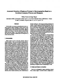
Figure 1: (a) Mammogram Image, (b) Segmented Image Step 14. Compare this local minimum (Lmin) with the global minimum (Gmin), if Lmin is less than Gmin, assign Gmin = Lmin. Step 15. Select the ant, whose solution is equal to local minimum, to update its pheromone globally. Step 16. Perform the steps (13) to (15) till all the image pixels have been selected. Step 17. Perform the steps (7) to (16) for M times.
Step 18. The Gmin has the optimum label which minimizes the posterior energy function. Step 19. Store the pixels has the optimum label in a separate image, that is the segmented image.
3
Feature Extraction
Texture is one of the important characteristics used in identifying an object in an image [42]. The texture coarseness or fineness of an image can be interpreted as the distribution of the elements in the matrix. In this work, Surrounding Region Dependence Method (SRDM), GrayLevel Run-Length Method (GLRLM) and Gray Level Difference Method (GLDM) are used to extract the features from the segmented image. 3.1 Surrounding Region Dependence
Method (SRDM) The SRDM is based on a second-order histogram in two surrounding regions. Let us consider two rectangular windows centered on a current pixel (x,y) R1 and R2 are the inner surrounding region and the outer surrounding region, respectively. An image is transformed into a surrounding region-dependence matrix and the features are extracted for this matrix. In this method, two different regions of size 5×5 and 7×7 are selected for each pixel. And the number of pixels greater than the selected threshold value (q) is counted in each region. Let as assume m and n are the count from each region, the element in the surrounding region dependence matrix M(m,n) is incremented by 1. This procedure is repeated for all the image pixels and the matrix get updated. Normally a set of 5 different thresholds is selected such as 50, 60, 70, 80 and 100. A separate matrix is generated for each threshold value. The algorithm as follows: Step 1. Select the peak threshold value from the histogram of the mammogram. Step 2. Select a pixel, whose intensity value is greater than the selected threshold value. Step 3. Extract two sub regions R1 and R2, of size 5×5 and 7×7, by considering the selected pixels as center pixel. Step 4. Calculate the surrounding regiondependence matrix which is defined as, M(q) = [ α (i,j) ], 0 ≤ i ≤ m, 0 ≤ j ≤ n, Where q is the threshold value and m, n are the number of pixels in the regions R1 and R2. Step 5. The element α(i,j) is given as: α(i,j)=#{(x.y)|cR1(x,y)=i and cR2(x,y)=j,(x,y) ∈ Lx×Ly}, where
cR1(x,y)=#{(k.l)|(k,l)∈R1 and [ S(x,y) – S(k,l)] > q }, cR2 (x,y) = # { (k.l) | (k,l) ∈ R2 and [ S(x,y) – S(k,l)] > q }, where # denotes the number of elements in the set, S(x,y) is the intensity value of the current pixel (x,y). Step 6. From this surrounding region dependence matrix the following features are extracted. Step 7. Horizontal Weighted Sum HWS = ΣΣij j2 r(i,j) Step 8. Vertical Weighted Sum VWS = 1/N ΣΣij i2 r(i,j) Step 9. Diagonal Weighted Sum DWS =1/NΣm+nk2[ΣΣij i2 r(i,j)] Step 10. Grid Weighted Sum GWS = 1/N ΣΣij ij r(i,j), N is the total sum of elements, and r(i,j) is the reciprocal of the element, r(i,j) = 1 / α(i,j).
3.2 Spatial Gray-Level Dependence Method (SGLDM) Statistical methods use second order statistics to model the relationships between pixels within the region by constructing Spatial Gray Level Dependency (SGLD) matrices. The SGLDM is based on an estimation of the second-order joint conditional probability density functions p(i,j|d,θ) for θ = 0, 45, 90 and 135°. The function p(i,j|d,θ) is the probability that two pixels, which are located with an intersample distance d and a direction θ, have a gray level and a gray level i and j. The spatial relationship is defined in terms of distance d and angle θ. If the texture is coarse, and distance d is small, the pairs of pixels at distance d should have similar gray values. Conversely, for a fine texture, the pairs of pixels at distance d should often be quite different, so that the values in the SGLD matrix should be spread out relatively uniformly. Similarly, if the texture is coarser in one direction than another, then the degree of spread of the values about the main diagonal in the SGLD matrix should vary with the direction θ. Thus the directionality can be analyzed by comparing spread measures of SGLD matrices constructed at various distances d and direction θ. The estimated joint conditional probability density functions are defined as follows [21]: P (i,j | d, 0°)=# {(k.l), (m,n))∈(Lx×Ly)×(Lx × Ly); k=m, |l-n|=d, S(k,l)=i, S(m,n) = j }/T(d,0°) (4)
P(i,j|d,45°)=#{(k.l),(m,n))∈(Lx×Ly)×(Lx×Ly); k-m=d, l-n = -d, or k-m=-d, l-n = d S(k,l) = i, S(m,n) = j } / T(d,45°) (5) P (i,j | d,90°)=#{(k.l),(m,n)) ∈ (Lx×Ly)× (Lx×Ly); k-m=d, l=n, S(k,l) = i, S(m,n) = j } / T(d,90°) (6) P (i,j | d,135°)=#{(k.l), (m,n))∈(Lx×Ly)×(Lx×Ly); k-m=d, l-n =d, or k-m=-d, l-n = -d S(k,l) = i, S(m,n) = j } / T(d,135°) (7) where # denotes the number of elements in the set, S(x,y) is the image intensity at the point (s,y), k,l,m and n are the spatial coordinates, Lx and Ly are the dimension for SGLD matrices and T stands for the total number of pixel pairs within the image which have the intersample distance d and θ direction . The features are selected for various combinations of distance and theta values. 3.3 Gray-Level Run-Length Method
(GLRLM) The GLRLM is based on computing the number of gray-level runs of various lengths. A gray-level run is a set of consecutive and collinear pixel points having the same gray level value. The length of the run is the number of pixel points in the run. The gray-level run-length matrix is as follows: R(θ)=( g(i,j)|θ],0 ≤ i ≤ Ng, 0 ≤ j ≤ Rmax, (8) where Ng is the maximum gray-level and Rmax is the maximum length. The entropy textural feature of the mammogram image is measured. 3.4 Gray-Level Difference Method
(GLDM) The GLDM is based on the occurrence of two pixels which have a given absolute difference in gray level and which are separated by a specific displacement δ. For given displacement vector: δ = (∆x, ∆y) let S(x,y) = | S(x,y) - S(x+∆x,y+∆y) and the estimated probability-density function defined by D(i | δ) = Prob (S(x,y) = 1) (9) The next section describes the classification of extracted features from the textural analysis methods are classified using Backpropagation network (BPN) classifier.
4
Classifier
The classifier employed in this paper is a threelayer backpropagation neural network. The backpropagation neural network optimizes the net for correct responses to the training input data set. More than one hidden layer may be beneficial for some applications, but one hidden layer is sufficient if enough hidden neurons are used [22,44,56]. Initially the features extracted from the textural analysis method, are normalized between [0,1]. That is each value in the feature set is divided by the maximum value from the set. These normalized values are assigned to the input neurons. The number of hidden neurons is equal to the number of input neurons. And only one Input Neurons Wih Hidden Neurons
S1 Who
Output Neuron
S2
Figure 2: A Three-Layer Backpropagation Network output neuron. Initial weights are assigned randomly between [-0.5 to 0.5]. The output from the each hidden neuron is calculated using the sigmoid function, S1 = 1 / ( 1 + e-λx), (10) where λ=1, and x = Σi wih ki, where wih is the weight assigned between input and hidden layer, and k is the input value. The output from the output layer is calculated using the sigmoid function, S2 = 1 / ( 1 + e-λx), (11) where λ=1, and x = Σi who Si, where who is the weight assigned between hidden and output layer, and Si is the output value from hidden neurons. S2 is subtracted from the desired output. Using this error (d) value, the weight change is calculated as: (12) delta = d * S2 * ( 1 – S2). And the weights assigned between input and hidden layer and hidden and output layer are updated as: Who = Who + ( n * delta * S1); (13) (14) Wih = Wih + ( n * delta * k), where n is the learning rate, k is the input values. Again calculate the output from hidden and output neurons. Then check the error (d) value,
Extract the features Normalize the feature values between 0 to 1 Assign the feature values to input neurons Initialize the weights randomly between –0.5 to 0.5 Calculate the output from hidden (S1) and output (S2) neurons Calculate the delta = d * S2 * ( 1 – S2) Update the weights: Who = Who + ( n * delta * S1); Wih = Wih + ( n * delta * k) Perform the steps till the target output is equal to the desired output. Figure 3: Flowchart for BPN Classifier and update the weights. This procedure is repeated till the target output is equal to the desired output. The network is trained to produce a 0.9 output value malignant and 0.1 output value for benign. The classification performance was also studied by the jack-knife method and round-robin method (leave-one-out method) and the results were analyzed by using ROC analysis.
5
Receiver Operating Characteristic (ROC) Analysis
Diagnostic tests have particular importance in medicine, where early and accurate diagnosis can decrease the morbidity and mortality of disease. For many years, diagnostic performance was reported by the accuracy of test. The test accuracy is the percentage of the diagnostic decisions that turned out to be correct and very important for both quality of care and cost containment [58]. To evaluate the performance of BPN classifier, Receiver operating characteristic (ROC) analysis is performed. ROC analysis was employed to evaluate the performance of the texture-analysis methods in classifying the ROI’s into positive and negative ROI’s [23,39,40,50]. It is based on statistical decision theory and first developed in signal
detection theory [55]. ROC analysis was first used in medical decision making [36,37,38]. Subsequently, it was used in medical imaging. An ROC curve is a plot of operating points that can be considered as a plotting of true positive as a function of false positive. When we design a computer-aided diagnosis system, generating operating points is usually done by applying thresholds to the detection algorithm outputs that roughly correspond to the concept of confidence thresholds used by human observers. Most statistical classifiers produce outputs that can be easily threshold to generate a large number of operating points. A higher ROC, approaching the perfection at the upper left hand corner, would indicate greater discrimination capacity. The area under the ROC curve is an important criterion for evaluating diagnostic performance [39,50]. Usually it is referred as the AZ index. The AZ value of ROC curve is just the area under the ROC curve. The value of AZ is 1.0 when the diagnostic detection has perfect performance, which means that TP rate is 100% and FP rate is 0%. The estimation of the AZ value can be obtained with the trapezoidal rule that can underestimate areas under the curve. More operating points are generated; less underestimation error will be obtained. The AZ value can also be computed by fitting a continuous binomial curve to the operating points [39]. Figure 4 shows the ROC curves for comparison of classification performances for the texture analysis methods. The optimal parameters for each textureanalysis method were analyzed. Fig. 4 shows the values for various parameters. Each value is the average performance from ten combinations of training and testing pairs. Fig. 4(a) shows values for the SRDM with respect to the threshold q and the number of hidden neurons. The optimal performance was achieved when q was 70 and the number of hidden neurons was six. In general, the larger the value of q, a large number of positive ROI’s can be classified as negative, whereas the smaller the value of q, a large number of negative ROI’s can be classified as positive. Fig. 4(b) and (c) shows the Az values for the SGLDM and the GLDM with respect to the intersample distance d and the number of hidden neurons. The optimal performances were achieved when d was one and the numbers of hidden neurons are ten and seven for the SGLDM and the GLDM, respectively. The performance decreases as the intersample distance
d increases. Fig. 4(d) shows the results of Az values for the GLRLM with respect to the number of hidden neurons. The optimal performance was achieved for eight hidden neurons. 1
1
d=1 d=3 d=5 d=7
0.9
0.9
0.8
Az
Az
0.8
0.7
0.7 q=50 q=70 q=100
0.6
q=60 q=80
0.6 0.5
0.5 0
2
4
6
8
10
0
12
2
4
6
8
10
12
N um be r of H idde n N e urons
N umbe r of H idde n N e urons
(b) SGLDM
(a) SRDM
1
0.9
0.9
0.8
0.8
Az
Az
1
0.7
d=1 d=3 d=5 d=7
0.7 0.6
0.6 0.5
0.5 0
2
4
6
8
10
12
N umbe r of H idde n N e urons
0
2
4
6
8
10
12
N umbe r of H idde n N e urons
(d) GLRLM (c) GLDM Figure 4: Comparisons of classification performances for the texture-analysis methods
6
Results
The backpropagation neural network is tested by using a jack-knife method [57] and a round-robin method [42]. The results were analyzed by using ROC analysis [23]. ROC analysis was employed to evaluate the performance of the textureanalysis methods in classifying the benign and malign. The area under the ROC curve, Az, was used as a measure of the classification performance.
6.1 Jack-Knife Method The classification performance was first studied using the jack-knife method and ROC analysis. For the jack-knife method, one half of the sample patterns were selected randomly from the database for training of the neural network; subsequently, the other half of the sample patterns were used for testing the trained neural network [42]. In this work, ten combinations of training and testing pairs were used to generate the ROC curves. The training set was used to train the backpropagation algorithm. Each training in this
is repeated in this manner until all samples have been used once as a test sample. The performance comparison using the round-robin method was performed with the optimal parameters, which were defined by the jack-knife method.
experiment was completed once the value of the error is less than 0.1. The learning rate and the momentum had values of 0.08 and 0.7, respectively. Fig. 5 shows a comparison of the four ROC curves obtained by using the optimal parameters for each of the four texture analysis methods. TPF and FPF denote the true-positive fraction and the false-positive fraction, respectively. The values for the SRDM, the SGLDM, the GLDM, and the GLRLM are 0.94, 0.90, 0.76, and 0.70, respectively. The textural features from the SRDM have the best performance in terms of the area under the ROC curve, Az, whereas those of the GLRLM have the worst performance. 6.2 Round-Robin Method The classification performance was also studied by the round-robin method (leave-one-out method) and ROC analysis. For P sample patterns, the round-robin method trains the classifier with P-1 samples, and then uses the one remaining sample as a test sample. Classification
Fig. 6 shows a comparison, based on the round-robin method, of the ROC curves for each texture-analysis method. The values for the SRDM, the SGLDM, the GLDM, and the GLRLM are 0.94, 0.89, 0.74, and 0.71, respectively. The textural features extracted from the SRDM have the best performance in terms of the area under the ROC curve, Az, whereas the GLRLM has the worst performance.
7
Conclusion
In this paper, we have applied a novel approach to mammogram image segmentation and classification based on the combination of Markov Random Field, Ant Colony System with Genetic Algorithm, and Backpropagation Neural Network with ROC Analysis. In MRF the image pixels are labeled and their posterior function values are computed. Ant Colony Optimization (ACO) with Genetic Algorithm have been used to find out the optimum label that minimizes the Maximizing a Posterior estimate to segment the image. The ACO search is inspired by the foraging behavior of real ants. Each ant constructs a solution using the pheromone information accumulated by the other ants. In each iteration, local minimum value is selected from the ants’ solution and the pheromones are updated locally. Genetic Algorithm is used to find out the local minimum. If this value is less than global minimum, the local minimum is assigned to global minimum. The pheromone of the ant that generates the global minimum is updated. At the final iteration global minimum returns the optimum label for image segmentation. Finally the mammogram textural features are extracted from the segmented image and they are classified using Backpropagation Neural Network (BPN) classifier. The textural analysis method, such as Spatial Gray Level Dependence Method (SGLDM), Surrounding Region Dependence Method (SRDM), Gray Level Run-Length Method (GRLM) and Spatial Gray Level Difference Method (SGDM) are used to extract the features from the segmented image and compared. From the viewpoint of classification accuracy and computational complexity, the SRDM was superior to the other methods. The BPN classifier is trained using jack-knife method,
and Round-robin method. The results from the classifier are analyzed using Receiver Operating Characteristic (ROC) analysis. If the output is 0.9 the calcification is consider as malignant, if it is 0.1, the calcification is consider as benign. Under the Az curve the performance of the classifier is evaluated. The results shows that the Ant Colony System segments the microcalcifications better than the existing methods by producing the higher Az value that is 0.94 at SRDM based feature extraction. The detection rate can be improved further by applying feature selection algorithms to select the optimal features from the original feature set and consider this minimal set for classification. As an extension of this work we are experimenting with various meta-heuristic algorithms to select the optimal features.
[10] [11]
[12]
[13] [14]
[15]
Acknowledgement
[16]
The first author sincerely acknowledges the University of Grant Commission (UGC), New Delhi, India for extending the financial support under UGC Special Assistance Programme.
[17]
References [1] R. Beckers, J. L. Deneubourg, and S. Goss. Trails and
[2]
[3]
[4]
[5]
[6]
[7]
[8]
[9]
U-turns in the selection of the shortest path by the ant Lasius. niger. J. Theor. Bio., 159:397–415, 1992. S. Bothorel, B. B. Meunier and S. Muller. A fuzzy logic based approach for semiological analysis of microcalcifications in mammographic images. Int. J. Intelligent Systems, 12:819–848, 1997. G. A. Carpenter and N. Markuzon. ARTMAP-IC and medical diagnosis: Instance counting and inconsistent cases. Neural Networks, 11(2):323–336, 1998. H. D. Cheng, J. R. Chen, R. I. Freimanis and X. H. Jiang. A novel fuzzy logic approach to microcalcification detection. J. Inform. Sci., 1–14, 1998. A. Colorni, M. Dorigo, and V. Maniezzo. In F.J. Varela, P. Bourgine. Distributed optimization by ant colonies. Proceedings of the First European Conference on Artificial Life, Paris, 1991. J. Dengler, S. Behrens and J. F. Desaga. Segmentation of microcalcifications in mammograms. IEEE Trans. Med.Imag., 12(4):634– 642, 1993. S Detounis. Computer-Aided Detection and Second Reading Utility and Implementation in a HighVolume Breast Clinic, Applied Radiology, 8–15, 2004. M. Dorigo and L. M. Gambardella. Ant colonies for the traveling salesman problem. BioSystems, 43:73– 81, 1997. M. Dorigo and L. M. Gambardella. Ant Colony System: A cooperative learning approach to the
[18]
[19]
[20]
[21]
[22]
[23]
[24]
[25]
[26]
traveling salesman problem. IEEE Transactions on Evolutionary Computation,1(1):53-66, 1997. M. Dorigo and T. Stuztle, Ant Colony Optimization, PHI ed, 2005. M. Dorigo, V. Maniezzo and A. Colorni, Positive feed back as a search strategy, Technical Report (16) Politecnico di Milano, Italy, 1991. M. Dorigo, V. Maniezzo and A. Colorni. The Ant System: Optimization by a Colony of Cooperating Agents. IEEE Transactions on Systems, Man and Cybernetics-Part B, 1(26):29-41, 1996. R. O. Duda, and P. E. Hart. Pattern Classification and Scene Analysis. New York: Wiley, 1973. M. M. Galloway. Texture analysis using gray level run lengths. Comput. Graph. Image Processing, 4: 172–179, 1975. J. A. Gamez and J. M. Puerta. Searching for the best elimination sequence in Bayesian networks by using ant colony optimization. Pattern Recognition Letters, 23:261-277, 2002. Y. Ge, Q. C. Meng, C. J. Yan and J. Xu. A Hybrid Ant Colony Algorithm for Global Optimization of Continuous Multi-Extreme Functions. Proceedings of the Third International Conference on Machine Learning and Cybernetics, Shanghai, 2427-2432, 2004. F. Glover. Tabu search: a tutorial. Interfaces, 20:74– 94, 1990. D. E. Goldberg. Genetic Algorithms in Search, Optimization and Machine Learning, Addison Wesley Longman Pte. Ltd., 3rd ed. 60 – 68, 2000. S. Goss, S. Aron, J. L. Deneubourg, and J. M. Pasteels. Self-organized shortcuts in the Argentine ant. Naturwissenschaften, 76:579–581, 1989. M. Gudmundsson, E. A. El-Kwae and M. R. Kabuka. Edge Detection in Medical Images Using a Genetic Algorithm. IEEE Transactions on Medical Imaging, 17(3):469 – 474, 1998. R. M. Haralick, K. Shanmugan, and I. Dinstein. Textural features for image classification. IEEE Trans. Syst., Man, Cybern., vol. SMC-3:610–621, 1973. J. Herz, A. Krogh, and R. Palmer. Introduction to the Theory of Neural Computation. Reading, MA: Addison-Wesley, 1991. H. Jean, M. C. David, F. B. Charles, P. Zygmunt and J. D. Edward. Pre-clinical ROC studies of digital stereomammography. IEEE Trans. Med. Imag., 14(2):318–327, 1995. H. R. Jin. Extraction of microcalcifications from mammograms using morphological filter with multiple structuring elements. System Comput. Jpn., 24(11):66–74, 1993. N. Karaboga, A. Kalinli and D. Karaboga. Designing digital IIR filters using ant colony optimization algorithm. Engineering Applications of Artificial Intelligence, 17:301–309, 2004. N. Karssemeijer. A stochastic model for automated detection of calcifications in digital mammograms. 12th International Conference IPMI, Wye, UK, 227– 238, 1992.
[27] N. Karssemeijer. Adaptive noise equalization and
[45] D. Rumelhart, G.E. Hinton, and R.J. Williams, D.E.
image analysis in mammography. Information Processing in Medical Imaging: 13th International Conference, IPMI ’93, AZ, USA, 472–486, 1993. C. Kervrann and F. Heitz. A Markov Random Field Model-Based Approach to Unsupervised Texture Segmentation Using Local and Global Statistics. IEEE Transactions on Image Processing, 4(6): 856 – 862, 1995. J. K. Kim, J. M. Park, S. S. Song and H. W. Park. Detection of clustered microcalcifications on mammograms using surrounding region dependence method and artificial neural network. J. VLSI Signal Process., 18: 251–262, 1998. S. Kirkpatrick, D. Gelatt, and M. P. Vecchi. Optimization by simulated annealing. 220:671–680, 1983. P. A. Lachenbruch, Discriminant Analysis. New York: Hafner, 1975. F. Lefebvre, H. Benali, E. Kahn and R. D. Paola. A fractal approach to the segmentation of microcalcifications in digital mammograms. Med. Phys., 22(4):381–391, 1995. H. D. Li, M. Kallergi, L. P. Clarke, V. K. Jain and R. A. Clark. Markov Random Field for Tumor Detection in Digital Mammography. IEEE Transactions on Medical Imaging, 14(3):565 – 576, 1995. H. Li, K. J. R. Liu and S. C. B. Lo. Fractal modeling and segmentation for the enhancement of microcalcifications in digital mammograms. IEEE Trans. Med. Imag., 16(6):785–798, 1997. H. Li, K. J. R. Liu and S. C. B. Lo. Fractal modeling of mammogram and enhancement of microcalcifications. IEEE Nuclear Science Symposium & Medical Imaging, 3:1850–1854, 1996. L. B. Lusted. Decision-making studies in patient management, N. Engl. J. Med., 284:416–424, 1971. L. B. Lusted. Introduction to Medical Decision Making. Thomas, Springfield, IL, 1968. L. B. Lusted. Signal detectability and medical decision-making. Science, 171:1217–1219, 1971. J. L. Maria, G. T. Pablo, S. Miguel, J. M. Arturo and J. V. Juan. Real and simulated clustered microcalcifications in digital mammograms: ROC study of observer performance. Medical. Physics., 24(9):1385–1394, 1997. C. E. Metz. ROC methodology in radiologic imaging. Invest. Radiol., 21(9):720–733, 1986. J. M. Mossi and A. Albiol. Improving detection of clustered microcalcifications using morphological connected operators. IEEE Image Processing and its Applications, 498–501, 1999. M. Nadler and E. P. Smith. Pattern Recognition Engineering. New York: Wiley, 1993. N. Pandey, Z. Salcic and J. Sivaswamy. Fuzzy logic based microcalcification detection. Neural Networks for SignalProcessing—Proceedings of the IEEE Workshop, 2:662–671, 2000. W. Qian, L. P. Clarke, M. Kallergi and R. A. Clark. Tree-structured nonlinear filters in digital mammography. IEEE Trans. Med. Imag,, 13(1):25– 36, 1994.
Rumelhart, Parallel and Distributed Processing. Cambridge, MA: MIT Press, 1986. L. Shen, R. Rangayyan, J. E. L. Desautles. Detection and classification of mammographic calcifications. Int. J. Pattern Recognition Artif. Intell., 7:1403–1416, 1993. J. Siddiqui, M. Anand, K Mehrotr, R. Sarangi and N. Mathur. Biomonitoring of Organochlorines in Women with Benign and Malignant Breast Disease. Environmental Research, 1-8, 2004. A. Speis and G. Healey. An Analytical and Experimental Study of the Performance of Markov Random Fields Applied to Textured Images Using Small Samples. IEEE Transactions on Image Processing, 5(3): 447 – 458, 1996. R. N. Strickland and H. I. Hahn. Wavelet transforms for detecting microcalcifications in mammography. Proceedings of the International Conference on Image Processing, 402–406, 1994. J. A. Swets. ROC analysis applied to the evaluation of medical imaging techniques. Invest. Radiol., 14(2): 109–121, 1979. K. Thangavel, M. Karnan, R. Siva Kumar, and A. Kaja Mohideen. Automatic Detection of Microcalcification in Mammograms-A Review. International Journal on Graphics Vision and Image Processing, 5(5):31-61, 2005. K. Thangavel and M. Karnan. Computer Aided Diagnosis in Digital Mammograms: Detection of Microcalcifications by Meta Heuristic Algorithms. International Journal on Graphics Vision and Image Processing, 7, 2005. (Article in Press). W. J. H. Veldkamp and N. Karssemeijer. An improved method for detection of microcalcification clusters in digital mammograms. The SPIE Conference on Image Processing, 3661:512–522, 1999. C. J. Vyborny and M. L. Giger. Computer vision and artificial intelligence in mammography. Am. J. Roentgenol., 162:699–708, 1994. A. Wald. Statistical Decision Functions, Wiley, New York, 1950. P. J. Werbos. Beyond regression: New tools for prediction and analysis in the behavioral sciences, Ph.D. dissertation, Harvard Univ., Cambridge, MA, 1974. J. S. Weszka, C.R. Dyer, and A. Rosenfeld. A comparative study of texture measures for terrain classification. IEEE Trans. Syst., Man, Cybern., SMC-6: 269–285, 1976. M. H. Zweig and G. Campbell. Receiver-operating Characteristic (ROC) Plots: A Fundamental Evaluation Tool in Clinical Medicine. Clinical Chemistry, 39:561-577, 1993.
[28]
[29]
[30]
[31] [32]
[33]
[34]
[35]
[36] [37] [38] [39]
[40] [41]
[42] [43]
[44]
[46]
[47]
[48]
[49]
[50]
[51]
[52]
[53]
[54]
[55] [56]
[57]
[58]
The following author designated as corresponding author:
Name: Karnan Marcus, E-mail id:
[email protected], Postal Address: 153, Palayam, Palani, Dindigul Dt, Tamil Nadu, India – 624601. Fax.No:91-4551-227229,91-4551-227230, Telephone.No:91-4551-227229,91-4551-2272