Automatic Identification of Discourse Markers in ... - Semantic Scholar

Automatic Identification of Discourse Markers in Dialogues: An In-Depth Study of Like and Well Andrei Popescu-Belis∗,a , Sandrine Zuffereyb a Idiap

Research Institute, PO Box 592, 1920 Martigny, Switzerland of Linguistics, University of Geneva, 1211 Geneva 4, Switzerland

b Department

Abstract The lexical items like and well can serve as discourse markers (DMs), but can also play numerous other roles, such as verb or adverb. Identifying the occurrences that function as DMs is an important step for language understanding by computers. In this study, automatic classifiers using lexical, prosodic/positional and sociolinguistic features are trained over transcribed dialogues, manually annotated with DM information. The resulting classifiers improve stateof-the-art performance, at about 90% recall and 79% precision for like (84.5% accuracy, κ = 0.69), and 99% recall and 98% precision for well (97.5% accuracy, κ = 0.88). Automatic feature analysis shows that lexical collocations are the most reliable indicators, followed by prosodic/positional features, while sociolinguistic features are marginally useful for the identification of DM like. The differentiated processing of each type of DM improves classification accuracy, suggesting that these types should be treated individually. Key words: discourse markers, discourse marker identification, statistical classifiers, lexical features, prosodic features

1. Introduction Discourse markers (henceforth, DMs) are linguistic items that play an important role in the interpretation of utterances, despite being relatively devoid of proper grammatical function or semantic content. Many studies in linguistics and in language technology have observed that the same lexical items can sometimes be used as DMs but other times have non-discursive grammatical functions. For instance, the following utterance: This was like one of the first meetings I ever participated in can have two quite distinct interpretations: “this resembled . . .” vs. “this was approximately one of the first meetings I ever participated in.”1 In the first case, like is a preposition, while in the second case it is a DM. The choice of the correct interpretation depends on the role of like, which would typically be signaled prosodically or, in writing, by the use or not of commas surrounding the lexical item. In this study, we use machine learning techniques to solve the binary classification task underlying the identification of DMs like and well, which play numerous other roles when they do not act as DMs: for instance, the first one can also be a preposition or a verb, and the second one an adverb. We first introduce DMs from a linguistic and pragmatic perspective, emphasizing their importance for human language technology (Section 2), and review previous studies of DM identification (Section 3). We present our DM annotation for like and well over the ICSI-MR corpus (Janin et al., 2003) in Section 4, and discuss the features and classifiers used for DM identification in Sections 5 and 6. Our results improve over state-of-the-art performance and are comparable to inter-annotator agreement scores (Section 7). We finally analyze the relevance of various features (Section 8) and conclude that like and well exhibit distinct properties, and are therefore better identified using separate sets of features (Section 9). author (phone: +41 27 721 7729, fax: +41 27 721 7712). Email addresses: [email protected] (Andrei Popescu-Belis), [email protected] (Sandrine Zufferey) URL: http://www.idiap.ch/~apbelis (Andrei Popescu-Belis), http://www.unige.ch/lettres/linguistique/zufferey/ (Sandrine Zufferey) 1 The utterance is extracted from the ICSI-MR corpus (see Section 4.1), meeting Btr002, starting at 2,799 s, on channel 7. ∗ Corresponding

Preprint of article published in Computer Speech and Language, vol. 25, n. 3, p.499-518, 2011.

2. Importance and difficulty of DM identification 2.1. Characteristics of DMs The great diversity of approaches to DMs is reflected by the range of alternative names used to refer to them, e.g. discourse particles, discourse connectives, pragmatic markers, or cue phrases. Following Andersen (2001, page 39), we consider that DMs are “a class of short, recurrent linguistic items that generally have little lexical import but serve significant pragmatic functions in conversation.” Items typically featured in this class include, in English, actually, and, but, I mean, like, so, you know, and well, although the lists differ depending on authors, theoretical stances, and goals of the studies. For instance, Fraser (1990) put forward a list of 32 English DMs, but Schiffrin (1987) listed only 23, and these two lists have only five elements in common. Some lexical items can be used both as DMs, playing a pragmatic or discursive role, and as non-DMs, in a semantic or sentential role. The following list of properties identified by Schourup (1999) characterizes the discursive roles: connectivity, optionality, non-truth-conditionality, weak clause association, initiality, orality, and multi-categoriality. For instance, in the example of our introduction, DM like is optional, is not syntactically bound, does not affect the truth conditions of the statement, and is typical of spoken utterances – though it is not initial, and does not function as a connective. In other cases, other subsets of properties can be more prominent. Two kinds of multi-functionality (hence, of ambiguity) must be distinguished: type-related vs. token-related, or sequential vs. simultaneous (Petukhova and Bunt, 2009). The first kind concerns lexical items that are sometimes used as DMs and sometimes as non-DMs, as are like and well, and could be due to the grammaticalization process which often licenses DM uses (Traugott, 1995; Romaine and Lange, 1991), or to the polysemous nature of DMs (Pons Border´ıa, 2008). The second kind refers to an occurrence of a DM that functions in several discourse-related domains, such as rhetorical or interpersonal, as theorized for instance by Schiffrin (1987) or Hovy (1995) and observed by Petukhova and Bunt (2009) on meeting transcripts. The target of the present study is sequential multi-functionality, i.e. deciding for each occurrence whether it functions as a DM or a non-DM, focussing on two particular lexical items, like and well. 2.2. Use of DMs in speech and language processing Language technology must deal with DMs because of their high frequency, especially in spoken language. Once they are identified, two main processing strategies can be adopted: deletion or exploitation. In speech processing, DMs are a type of disfluency often equated to lexicalised filled pauses, and are therefore generally removed before parsing an utterance, although their role for managing the communication has been recognized.2 In their work on parsing disfluent speech, Lease and Johnson (2006) found that cleaning up disfluencies increased parser performance, but mainly for parsers trained on out-of-domain data. Core and Schubert (1999) argued that disfluency information, including DMs, should instead be “conveyed to higher-level reasoning processes”, and hypothesized that making a parser aware of disfluency information could allow it to “correct errors made in pre-parser repair identification”. Alternatively, the presence of DMs was often used to infer information about the extent and role of utterances, as summarized by Hirschberg and Litman (1993, Table 14, pages 529–530) and Samuel (1999, Section 6.2.1). When used to infer the structure of discourse, DMs were often referred to as discourse connectives, or cue/clue words. For instance, in Reichman’s study (1985, see page 188), clue word classification directed the interpretation of utterances, e.g. an initial because or like were considered to signal a support move. A successful discourse parser for written text was designed by Marcu (2000), making use of DMs among other indicators of rhetorical relations between discourse segments. In the Penn Discourse Treebank corpus, discourse relations were manually annotated based on explicit or implicit discourse connectives from about 100 types (Prasad et al., 2008). In all these studies, like was seldom categorized as a connective, while well sometimes was, but the potential ambiguity of the candidate DMs was not considered. DMs have been used to infer discourse information on a lower structural level, notably for the segmentation of spoken discourse into utterances (Stolcke et al., 1998; Passonneau and Litman, 1997; Heeman and Allen, 1999) or 2 Brennan and Schober (2001) showed that their presence improved understanding of spoken instructions, compared to silent pauses, while Jones et al. (2003) found that automatic disfluency removal degraded the readability of the automatic speech recognition output (although manual removal improved the readability of manual transcripts).

2

for the recognition of dialogue acts (Samuel, 1999; Byron and Heeman, 1997). Applications to the improvement of speech recognition have been considered as well: Heeman and Allen (1999) used an enriched statistical language model that included POS tags, DMs, speech repairs and intonational phrases, thus reducing POS errors by 2.5%, and decreasing perplexity by a small amount too (Heeman and Allen, 1999, page 18). Byron and Heeman (1997) studied utterances starting with one of the four following DMs: and, so, well, oh, and showed that DM use is somewhat correlated with the type of conversational moves. In a pilot study on two meetings of the ICSI-MR corpus, it was found that turn-initial so was more frequently used by meeting leaders in topic-relevant utterances, and was also used as a floor grabber (Janin et al., 2004, Section 4.3). 2.3. Like and well as DMs or non-DMs Like and well are among the most frequent and ambiguous lexical items that can serve as DMs, which makes their study both challenging and potentially rewarding, in terms of generality and insights for other DM identification tasks. Schourup’s (1985) book on common discourse particles is entirely dedicated to like, well, and you know, while in Samuel’s (1999, Appendix F) survey of cue phrases from thirteen significant articles or books, well is quoted in eight of them and like in five. Both lexical items were included in all previous studies of DM identification (see Section 3), though not always in studies of disfluency correction. Like has a large number of possible functions, in DM as well as non-DM roles. When it is not used as a DM, like can be a preposition, a conjunction, or a verb, but also a noun, an adjective, or an adverb. As a DM, like may function as a lexicalised filled pause, akin to an interjection or hesitation word such as uhmm, uttered while preparing the upcoming words of the utterance. But like often fulfils more complex roles in dialogue, broadly indicating to the hearer that what follows it is a loose interpretation or an approximation of the speaker’s belief (Andersen, 2000, 2001). Five different functions of the DM like have been identified in the literature, and are illustrated below by excerpts from the ICSI-MR corpus, with added punctuation. In (1), like indicates an approximation or hedge; in (2), it introduces an example; in (3), the approximation concerns the form of the expression rather than its content: in (4), like introduces a correction; and in (5) a quotation or reported speech.3 1. We just came up here one night after recording, so it took, like, twenty minutes – something like that. (Bmr001, 276 s, c8) 2. Those are the two options: either, like, make an arrow directly, or put a new node. (Bed003, 2,282 s, c3) 3. I was at this place in Europe where they had little carvings of, like, dead people on the walls or something. (Bed003, 292 s, c2) 4. It might be that if you add a new thing pointing to a variable you just, like. . . it just overwrites everything. (Bed003, 1,608 s, c3) 5. And he was like, yeah, I can make dogs, uh, raise their ears. (Btr002, 2,423 s, c9) Similarly, well can fulfil a variety of pragmatic and non-pragmatic functions. When it is not a DM, well can be an adverb or an adjective, but also – due to homography – a noun or even a verb, although no such instances were found in the ICSI-MR corpus. As a DM, the role of well is, broadly speaking, to “signal that the context created by an utterance may not be the most relevant one for the interpretation of the next utterance” (Jucker, 1993, page 450). Four specific functions of the DM well have been identified in the literature (Jucker, 1993; Schourup, 2001; de Klerk, 2005), again illustrated below with examples from the ICSI-MR corpus. In (6), well conveys some kind of insufficiency, showing that a background assumption of speaker A is not entirely adequate, and B cannot answer A’s question without denying that assumption first; in (7), well is a “face-threat mitigator” which helps to disagree politely; in (8), well introduces an instance of reported speech, while in (9) it marks hesitation. 6. A: Is the rising pitch a feature? Or is it gonna be in the same file? (Bdb001, 1,474 s, c3) B: Well, the rising pitch will never be hand-annotated. (Bdb001, 1,478 s, cB) 7. A: We’d need to prune. Right? Throw things away. (Bed012, 493 s, c2) B: Well, actually, you don’t even need to do that with XML. (Bed012, 495 s, c3) 3 The quotative function of DM like is in fact one of its most recent pragmatic functions, dating from the 1970s or 1980s (Schourup, 1985; Andersen, 2001, page 294), and could represent “a case of grammaticalization in process” (Romaine and Lange, 1991).

3

8. So, they’ll say, well, these are the things I want to do. (Bed006, 533 s, cA) 9. Oh, yes, but – well, uh, yes, but what I mean is that, uh, from the transcriber’s perspective, uh, those two functions are separate. (Bmr008, 794 s, c8) 3. Automatic identification of DMs: previous studies DM identification modules are seldom implemented, as Heeman and Allen observed (1999, p. 40): “although numerous researchers have noted the importance of DMs in determining discourse structure, there has not been a lot of work in actually identifying them.” This may be due to the fact that many DMs, often acting as discourse connectives, are not as ambiguous as like or well. In this section, we summarize the main methods and findings of the studies that have explicitly focused on the problem of DM identification. For comparison with our results, their scores are gathered in Table 8 at the end of the article. 3.1. Hirschberg and Litman (1993) Hirschberg and Litman (1993) proposed the first method for DM identification based on prosodic information, building upon an initial study of now and well in the recording of a radio show. The method consisted in sets of rules (called “models”) to distinguish DM vs. non-DM occurrences: e.g., a token in the initial position of a multi-word phrase that is deaccented or has a low intonational tone is likely to be a DM. For each candidate DM, the prosodic features required by the rules were extracted manually. An alternative model was based only on “orthographic” cues from a manual transcript: commas, periods, dashes and paragraph breaks. The models were tested on 878 tokens of candidate DMs, corresponding to 34 types, including like and well, on which annotators agreed. The prosodic model correctly classified 75.4% of the tokens, with κ = 0.52, 63.1% recall and 88.3% precision for DM retrieval – as computed by Heeman (1997, p. 58–60)). The accuracy increased to 85.3% when coordinate conjunctions (and, or, but) were excluded from the count leaving only 495 tokens, with κ = 0.69, 82.7% recall and 81.5% precision. The orthographic model correctly classified 80.1% of the 878 tokens, with κ = 0.54, 57.3% recall and 82.6% precision, scoring higher than the intonational one thanks to the correct punctuation entered by human annotators. 3.2. Siegel and McKeown (1994) Siegel and McKeown (1994) proposed a transcript-based method for DM identification using decision tree classifiers. Unlike the hand-coded models cited above, the decision trees were optimized by a genetic algorithm. Similarly to Hirschberg and Litman’s orthographic model, the features used by the decision trees were the type of the candidate DM (i.e. the lexical item) and the tokens immediately preceding and following it (the tokens situated 2, 3 or 4 words after it appeared not to be useful). Over a superset of Hirschberg and Litman’s data with 1,027 tokens, the classification accuracy of the best decision tree found in this study was 79.20%, but a simple rule found by the authors (“all utterance-initial candidates are DMs”) scored almost as high, at 79.16% accuracy. The authors did not provide confusion matrixes, therefore recall, precision and κ cannot be computed. A number of linguistic rules were inferred from the decision trees constructed automatically, for instance the use of constructs such as the like or as well to disambiguate the candidate DM. 3.3. Litman (1996) Litman (1996) extended earlier studies by refining manually-derived classification models, over the same data set, by training C4.5 decision trees, and by using the cgrendel algorithm to construct conditional rules, with similar results. The study used prosodic features assigned by human annotators, textual features extracted from human transcripts, POS information assigned automatically, and the type of the candidate DM. The prosodic features were the length and the position of the candidate in the intonational and intermediate phrase, the composition of the intermediate phrase, and the prosodic accent, in detailed or in abstracted form. The textual features were mainly indicators of the preceding and following punctuations and cue phrases. Curiously, the neighboring words were not used, despite Siegel and McKeown’s encouraging results. Overall, most of the prosodic and textual classifiers learned automatically outperformed corresponding models defined a priori by humans. The best performance using all available features was 83.1% accuracy (or 16.9% error 4

rate) on the whole set of 878 tokens, and 83.4% on the 495 non-conjuncts. The 95% confidence intervals, computed using 10-fold cross-validation, were respectively ±3.4 and ±4.1, but confusion matrixes were not provided, so recall, precision or κ cannot be computed. The best overall scores were however obtained by a classifier using only phraserelated prosodic features (excluding accent) and the identity of the candidate DM: 14.5%±3.3 error rate (85.5% accuracy), and 12.6%±3.3 on the non-conjuncts. The most useful features were not identified, but the POS and the following words or punctuations did not seem to increase performance. Specific processing of each type improved performance when prosodic and textual features were used, thus corroborating Siegel and McKeown’s findings. 3.4. Heeman et al. The problem of DM identification was coupled to speech recognition, utterance segmentation, POS tagging and repair detection and correction by, with the overall goal of increasing the accuracy of automatic speech recognition over the Trains corpus (Heeman, 1997; Heeman and Allen, 1999). DMs received one of the following POS tags: acknowledgment, discourse conjunct, discourse adverbial, and interjection. Decision tree classifiers for POS and DM were trained using features characterizing previous tags, but no acoustic features apart from pauses in speech. More than 35 DM types were considered, with 8,278 DM tokens, but no figure is given for the number of non-DM uses of the same lexical items. As the study aimed at the recognition of DMs rather than the disambiguation of DM candidates, the performance metrics were modified accordingly. As a result, κ and overall error rate cannot be deduced, because the total number of DM candidates is unknown. The best results of the language model correspond to 533 errors of DM identification, or to a 6.44% error rate, with 97.26% recall and 96.32% precision. The high recall and precision and low error rate are probably due to the high proportion of unambiguous markers in the data, as 1/7 of words are considered as DMs. 3.5. Studies on the disfluency-annotated Switchboard data Another line of research has studied the identification of DMs as a specific type of disfluencies, namely lexicalized filled pauses, in the Switchboard corpus of telephone conversations (see also Section 4.3). To clean up utterances in preparation for dialogue summarization, Zechner (2002) trained a rule-based POS tagger enriched with tags for disfluencies using lexical features. Detection of DMs reached 95% precision with 90% recall ( f = 0.93) on one third of Switchboard that was not used for training (5,787 DMs), but dropped to f = 0.30 on a test corpus of transcribed meeting fragments with 2,355 words. Similarly, Snover et al. (2004) used lexical features (words and POS tags) in a rule-based disfluency tagger, achieving 18.1% error rate (insertions and deletions) for DMs on clean conversation transcripts, and 6.5% on broadcast news ones. A rule-based model for detecting fillers, including DMs, was designed by Johnson et al. (2004) as a component for a rich transcription system. To reach their final score of 19% error rate on DMs, they focused on frequent DMs only and searched empirically for the most efficient lexical or POS indicators: for instance, like preceded by something or you or sound, or followed by that, was labeled as a non-DM; similarly, like followed by ‘VB’ or preceded by ‘NN’ was labeled as a non-DM. 4. Description of the data and its annotation 4.1. Corpus, speakers, and frequencies The ICSI-MR corpus of multi-party conversations comprises 75 meeting recordings, with five to eight speakers each (Janin et al., 2003). The meetings featured discussions about language processing and computer science, and involved native and non-native English speakers. The speech input was recorded through individual audio channels, which were manually transcribed. The recordings amount to about 80 hours and about 800,000 words, including 4,519 occurrences of the token like and 4,136 of well. Each channel was segmented into utterances (a total of 110,537), which were later annotated with dialogue act information (Shriberg et al., 2004). Word-level timing was generated using automatic alignment of the manual transcripts with automatic ones, and indications of interruptions and unfinished utterances were annotated as well.4 4 A study of DM so was announced on the ICSI-MR corpus, targeting its role as a DM indicating “important utterances” (Janin et al., 2004, Section 4.3). Two meetings were studied in detail, but to the best of our knowledge no large-scale annotation of DMs was carried out.

5

Table 1: Contributions to the ICSI-MR corpus – 52 speakers, 793,754 words, 110,537 utterances – sorted by mean length of utterance (MLU).

Feature

Value

Gender

female male non native native UK US West other countries other US US East undergraduate PhD graduate professor

Proficiency Origin

Education

Nb. of speakers 13 39 25 27 2 7 25 14 4 4 21 21 6

Nb. of words 22% 78% 26% 74% 1% 12% 26% 32% 28% 2% 40% 30% 28%

Nb. of utterances 23% 77% 28% 72% 2% 14% 28% 32% 24% 2% 42% 31% 25%

MLU 7.1 7.2 6.8 7.3 5.4 6.4 6.8 7.2 8.2 5.7 6.7 7.0 8.3

A total of 52 speakers contributed to the corpus, and submitted sociolinguistic information after the recordings: gender, age, education level, proficiency in English (native or non-native), region of origin, and influences of other languages (Table 1). The seven most frequent speakers contributed more than 40,000 words each (64% of the corpus), while the ten least frequent ones contributed less than 1,000 words each. As a result, given that only a few speakers produced most of the data, nearly all the speaker-related parameters are correlated when weighted by the number of words. In addition, the region of origin is correlated with age and education level, because speakers from the US East were on average older and had a higher education level than those from the US West. 4.2. Reference annotation of DMs A study of inter-annotator agreement on the DM identification task was performed, in two conditions, as a preliminary to the annotation of the entire amount of data (Zufferey and Popescu-Belis, 2004). The first condition involved six human annotators, three male and three female, aged 25 to 40, of which three were native English speakers and the three others had a very good command of English. Each person annotated utterances containing the token like from two different sources: 26 utterances from movie subtitles (American English from Pretty Woman) and 49 utterances corresponding to one meeting from the ICSI-MR corpus. The amount of tokens was thus similar to the one annotated in Hirschberg and Litman’s study, which had 61 occurrences of like in the test corpus (1993, Table 5, page 517), and comparable amounts of now and well in their pilot studies. The annotators had to decide for each occurrence of like whether it was a DM or not, based on written instructions concerning the roles of like as a DM, as well as examples of DM and non-DM uses, similar to those given in Section 2.3 above. Annotators were also asked to specify their degree of certainty on a three-point scale (hesitating, reasonably sure, or certain). In the second condition, three annotators were asked to annotate 55 occurrences of like from an ICSI-MR meeting, while being allowed to listen to the audio recording via a hypertext transcript synchronized to the audio files. The instructions were enriched with explanations about the prosody of like as a DM. Inter-annotator agreement was quite low, in the first condition, for the ICSI-MR corpus (κ = 0.42), and almost acceptable for the movie dialogues (κ = 0.65) according to Krippendorff’s scale (see Section 6). In the second condition, with prosodic cues, inter-annotator agreement increased to κ = 0.74, a value that qualified this task as empirically valid. The necessity of prosodic information thus confirms previous results (Grosz and Hirschberg, 1992; Hirschberg and Nakatani, 1996). Native and non-native English speakers reached similar levels of inter-annotator agreement, for both types of data: κ = 0.67 vs. 0.63 for the movie, and κ = 0.40 vs. 0.43 for the ICSI-MR corpus. The confidence of the annotators did not appear to correlate with agreement scores, though it increased by ca. 30% when audio was available. For all our subsequent experiments, the full ICSI-MR corpus was annotated by both authors for about half of the data, and by one author only for the remaining half. Instances on which the authors disagreed or that were marked as 6

uncertain – about 0.5% of the total – were removed from the data, as in Hirschberg and Litman’s studies, who removed about 6% of their instances. As a result, our annotation is one of the largest resources ever used in DM identification studies. 4.3. DM frequencies in the ICSI-MR and other corpora There are 4,519 occurrences of like in the ICSI-MR corpus, of which 2,052 serve as DMs (45.4%), and 4,136 occurrences of well, of which 3,639 serve as DMs (88.0%). The average frequency of DM like in the corpus is thus 0.26% of all words, and that of DM well is 0.46%. These two items are clearly among the most frequent DMs in this corpus, as it appears when comparing the word counts with a large list of DMs (e.g., Samuel, 1999). The most frequent candidate DMs are and, so and but, with respectively 18,074, 12,037 and 7,795 occurrences (as DMs or non-DMs), but their annotation is highly problematic and was not targeted here. These are followed by like and well, then closely by you know (with 4,096 occurrences), and with lower frequencies by then, I mean, because, actually and and so (3,703, 3,452, 2,106, 1,759 and 1,414 occurrences). The values for like and well in the ICSI-MR corpus are comparable to other values found for spoken English, though variation is quite large. Fuller (2003) counted the frequencies of six DMs among which like and well in an interview (ca. 24,000 words) and in an informal conversation (ca. 11,000 words), and found 0.55% and 0.62% for DM like, and respectively 0.36% and 0.55% for DM well. In a corpus of non-native English speakers, de Klerk (2005, p. 1189–1190) found 788 uses of well over 540,000 words, of which 494 (62.6% or 0.09% of all words) were DMs. In a 50,000 word sample of the London-Lund Corpus, we found 500 occurrences of well, of which 87.4% were DMs (0.87% of all words). The corpora used in previous studies of DM identification are generally much smaller. Hirschberg and Litman (1993) annotated 100 occurrences of now in the transcript of a radio show, of which 63 were DMs, and carried out another analysis on a corpus with 52 instances of well, of which 27 were DMs. Their main study was based on transcribed speech from a 75 minute keynote address at an AI conference in 1986, with ca. 12,500 words, and 953 occurrences of cue phrase candidates of 34 types. The most frequent token, and, occured 320 times, and 18 tokens occured less than 10 times each. Once the ambiguous tokens were excluded, the data had 878 tokens, of which 341 (38.8%) were DMs and 537 (61.2%) non-DMs. The same data containing 878 DM candidates was used by Litman (1996), and a superset of it with 1,027 occurrences was used by Siegel and McKeown (1994), with a new DM annotation that found 407 DMs (39.6%) and 620 non-DMs (60.4%). In the Switchboard corpus, five types of disfluencies were annotated: asides, empty coordinating conjunctions, editing terms, non-lexicalized filled pauses, and lexicalized ones, which were equated to DMs (Meteer et al., 1995). Under the broad definition of disfluencies as elements that must be removed to obtain grammatical sentences or at least constituents, DMs were viewed as having “more semantic content than fillers (although not always much)”, and a number of hints were given for the annotation of specific items: well, you know, like, so, and actually. Two main uses of like were considered, as a preposition or as a DM, and the difficulty for humans to distinguish between them based on the transcript only was acknowledged, especially when no commas were inserted. The disambiguation strategy proposed to annotators was: “if the speaker is a heavy discourse like user, count ambiguous cases as DMs, if not, assume they are not.” As for well, it was considered to be “common and easily recognized”, and annotators were instructed to use its presence to mark the beginning of an utterance. A total of about 32,500 DMs were thus annotated and subsequently used for training and testing automatic disfluency recognizers, among which 2,528 occurrences of DM (filler) like (22% of the total) and 9,761 occurrences of DM well (84% of the total). However, this annotated resource did not appear to be suitable for our present goal, as the annotation of like did not capture all its possible discourse functions, but only those akin to lexicalized filled pauses. For instance, the quotative uses of like were generally not annotated as DMs, with some exceptions, and as a result the proportion of DMs among all occurrences of like is much lower than for other data. Similarly, no discourse function was explicitly identified for well in the annotation instructions, although in this case the confusion between DM and filler uses had a smaller impact than for like. Heeman (1997) used transcripts of the Trains corpus with nearly 100 dialogues and 60,000 words, including 8,278 DMs. The data was POS tagged by human annotators, and DMs were annotated in this process as well. The number of annotators, the inter-annotator agreement, and the full list of DM types have not been published, and only examples from each class were shown (Heeman et al., 1998, Table 2). 7

Table 2: Counts and positional properties of DM vs. non-DM occurrences of like and well.

Type

Like

Well

Role DM non DM both DM non DM both

Occurrences 2,052 2,467 4,519 3,639 497 4,136

Utteranceinitial 342 92 434 2,755 10 2,765

completed utt. 9 69 78 117 208 325

Utterance-final interrupted utt. 138 58 196 249 2 251

total 147 127 274 366 210 576

Data with DM annotation is scarcer for languages other than English. In a corpus of transcribed conversations in Slovenian, Verdonik et al. (2007) annotated transcripts of 106 minutes of speech (15,517 words) with about twenty types of Slovenian DMs and their variants, finding 2,158 tokens. In an analysis of Dutch connectors, Penning and Theune (2007) counted DMs in a corpus of about 97,000 words, using sampling to estimate the frequency of lexical items that can serve as DMs or non-DMs. Samy and Gonz´alez-Ledesma (2008) designed a rule-based DM identification system and applied it to a 40,000 word Spanish corpus, resulting in 558 tokens of several dozen types, some of which had to be disambiguated manually. The annotation was then ported to the Arabic and English versions of the corpus, aligned with the Spanish one, using a set of manual heuristics. 5. Features for DM identification Our automatic method for disambiguating DM candidates relies on a variety of surface features which extend those used in previous studies: lexical collocations, prosodic properties, position in the utterance, and a set of sociolinguistic, speaker-related features. In addition, we use the type feature that distinguishes like from well, the dialogue act label of the utterance that contains the candidate DM, and the POS label assigned automatically by a tagger. 5.1. Lexical collocations In a previous study (Zufferey and Popescu-Belis, 2004), we have defined manually-defined collocation filters in order to restrict the set of candidate DMs based on the numerous linguistic studies that outlined frequent lexical collocations for DMs (see e.g. de Klerk, 2005, p. 1190). In the present study, we defined a range of possible lexical features, and allowed DM classifiers to make optimal use of them after learning over the training data. Two ways to encode lexical features were tested. The first representation used one variable for each word position relative to the DM candidate, that is, 2N variables noted word−N , word−N+1 , . . . , word−1 , word+1 , . . . , wordN−1 , wordN – the value of variable wordn being the word appearing in position n. These variables define a ‘lexical window’ of size 2N surrounding the DM candidate, restricted to words within the same utterance: if a position n lies outside it, then wordn is coded as absent. The second representation used one variable for each possible word, noted position(wordi ), indicating the position of this word with respect to the candidate DM: +1 if it is the following word, −1 if it is the preceding word, and so on. If the word is not present in a window of size 2N around the DM candidate, the value is set to zero by convention. Therefore, for each token, most variables will have the null value, except at most 2N ones. These two representations are conceptually equivalent, but are processed differently by machine learning algorithms. Moreover, if a given word has more than one occurrence in the lexical window, the second representation can encode only one of them: we chose by convention the closest one to the candidate, with priority to the occurrences following it. 5.2. Position and prosody Insights from previous studies show that position in the utterance and prosody are helpful features for DM identification. Fuller (2003, Table 9) found that like appeared mainly in turn- or utterance-medial positions, and well appeared 8

mainly in turn-initial positions, possibly following another DM, but almost never in utterance-medial positions. The position of a DM candidate in an utterance has often been used as a feature for DM identification (Hirschberg and Litman, 1993; Litman, 1996; Heeman and Allen, 1999). Not all the prosodic features are easy to extract automatically, so, for instance, Hirschberg and Litman (1993) used a manual annotation of prosodic accent. Moreover, several studies of disfluency identification – as for instance those cited by Zechner (2002, Section 5.3.3) in support of his own word-based approach – showed that prosodic information only brought a small increase in performance compared to models using words and turn boundaries. In the ICSI-MR corpus, the position of like and well within an utterance, as well as simple prosodic properties such as the duration, the pause before, and the pause after a candidate DM, can be obtained using the audio/transcript alignment and the utterance segmentation provided with the corpus (Janin et al., 2003; Shriberg et al., 2004). The positional properties of DMs vs. non-DMs are summarized in Table 2 above, showing that, for instance, like in an utterance-initial position has four times more chances to be a DM than a non-DM (342 vs. 92 instances), and that well ending an interrupted utterance is almost certainly a DM (249 vs. 2 occurrences). In addition, a comparison of the durations of like as DM vs. non-DM showed that either short (< 200 ms) or long (> 370 ms) occurrences of like are less likely to be DMs than occurrences around the average duration, possibly due to the different functions of non-DM like. 5.3. Sociolinguistic features Speaker-related information is potentially relevant to DM identification, e.g. if a class of speakers appears to have a marked preference for DM uses. Such preferences have already been observed by Meteer et al. (1995), who used them to guide human annotation, and by Snover et al. (2004), who used them to detect lexicalised filled pauses with ambiguous words such as like. The following linguistic features available with the ICSI-MR corpus (Table 1) have been explored: gender, age, education level, proficiency in English (native vs. non-native), and region of origin. For instance, we noted that DM like is preferred by speakers from the US West (0.50% of all produced words), as opposed to those from the US East (0.13%) or from other US regions (0.31%). DM like is also preferred by less educated speakers as opposed to more educated ones: for undergraduates, 1.26% of all their words are DM like, but only 0.33% for graduate students, 0.29% for speakers with a PhD, and 0.07% for professors. However, as age, region and education level are not independent in this data, their contribution to the overuse of DM like cannot by quantified separately. 5.4. Other features: part-of-speech and dialogue acts Part-of-speech (POS) information could help filtering out many of the non-pragmatic uses of like and well, on condition that the accuracy of POS taggers on speech transcripts is high enough, at least on the words surrounding the candidate DMs. However, the difficulty is that accurate POS tagging seems to require the recognition of DMs first. Indeed, according to Litman (1996, Table 6), adding automatically-assigned POS tags to the feature set did not increase performance with respect to the orthographic features. Johnson et al. (2004) found that using POS information of the tokens that were adjacent to lexicalised filled pauses increased scores by about 2% (absolute). Conversely, Heeman and Allen (1999, Table 7) found that the number of POS errors decreased by 2.5% when DMs were included in the language model, although the scoring metrics did not “penalize POS errors that result[ed] from a confusion between discourse and sentential usages.” We experimented with like on about half of the ICSI-MR corpus using QTag (Mason, 2000), a general-domain probabilistic POS tagger with the Brown/UPenn tagset. Occurrences of like received one of the following tags: preposition (IN, 1,412 occurrences), verb (VB, 509), subordinate conjunction (CS, 134), general adjective (JJ, 52), and general adverb (RB, 9). These do not map directly into the DM and non-DM classes, but were tested as indicators for filtering out non-DMs (Zufferey and Popescu-Belis, 2004). A simple filter that considered all VB as non-DM uses, and all others as (possible) DMs, had 0.77 recall, 0.38 precision, and a kappa of only 0.22. When adjectival uses of like (tagged JJ) were considered as potential DMs, recall was very low, but precision reached 0.74, showing that the JJ tag could be a better cue than VB. However, as these results are much lower than the scores of other features, these POS tags were not be used in our experiments. The main reason for the failure of the POS tagger to detect DM uses of like is probably that it was not trained on speech transcripts with proper punctuation. Here, we will not train a POS tagger on the ICSI-MR data, but our specific DM classifiers can serve as a pre-preprocessing device for POS tagging. 9

Finally, we also conducted experiments to assess the relevance to DM identification of manually-annotated dialogue act labels, which are available for the ICSI-MR corpus (Shriberg et al., 2004). Two representations of this information were tested: the labels were either used as provided, or decomposed into their constitutive elementary tags. 5.5. Summary of the features The information used by our automatic classifiers for each token (candidate DM) is summarized in the list below, with the name of each feature written in small capitals, followed by an enumeration of its possible values. The encoding of the lexical information was in addition determined by two parameters, which were optimized using the data: the size of the lexical window centered on the candidate DM (noted 2 ∗ N) and the cut-off frequency used to build the list of possible surrounding words W (only words appearing more than F times over all lexical windows were included in W). 1. Either (a) or (b) from the following representations: (a) word(−N), . . . , word(−1), word(+1), . . . , word(+N) – where word(n) ∈ W ∪ {‘absent’, ‘other’}; (b) position(wordi ) – for each wordi ∈ W, position(wordi ) ∈ {−N, −N + 1, . . . , 0, 1, . . . , N − 1, N}; 2. initial – set to ‘yes’ if the token is the first word of an utterance, to ‘no’ otherwise; 3. final – set to ‘yes-completed’ if the token is the last word of a completed utterance, to ‘yes-interrupted’ if it is the last word of an interrupted utterance, and to ‘no’ otherwise; 4. pause-before – the duration (in milliseconds) of the pause before the token, or set to 10 seconds if the utterance starts with the token; 5. pause-after – the duration (in milliseconds) of the pause after the token, or set to 10 seconds if the utterance ends with the token; 6. duration – the duration of the token itself (in milliseconds); 7. gender – ‘female’ or ‘male’; 8. age – age in years, rounded to an integer value; 9. education – ‘undergraduate’, ‘graduate’, ‘PhD’, or ‘professor’; 10. native – ‘native’ or ‘non-native’ English speaker; 11. origin – ‘UK’, ‘US East’, ‘US West’, ‘US other’, or ‘other’; 12. dialogue-act – the dialogue act label of the utterance containing the candidate, either as a whole, or decomposed into a list of elementary tags coded as separate features (first tag, second tag, etc.); 13. type – like or well, which allows a classifier to process the two lexical items differently, if the feature is available, or on the contrary requires a classifier to process them using the same rules, if it is not. 6. Training classifiers: methods and data Decision trees used for classification are made of nodes and branches: nodes represent the test of one feature of a DM candidate, and branches stand for the possible values of the tested feature. To each terminal node, or leaf, is associated one of the two possible classes, DM or non-DM. To determine whether a token is a DM or not, a classifier starts with the test appearing at the root node, and proceeds through the branches and successive nodes until a leaf is reached. Decision trees are explicit, easily interpretable classifiers, unlike support vector machines or neural networks. The higher a feature appears in an automatically-learned decision tree, the more general and discriminative it is. A feature will not appear in a tree if its correlation with the DM/non-DM distinction is not strong enough, or if it is superseded by more discriminative subsets of features. In our experiments, decision trees were trained using the C4.5 method (Quinlan, 1993), which optimizes trees in terms of the number of correctly classified instances. C4.5 implements several strategies to avoid local optima and speed up training. In particular, it is possible to: (1) search for binary trees only (two branches per node), and (2) require that each leaf classifies a minumum number of tokens (e.g. 5 or 20). We used the implementation of the C4.5 10

Table 3: Best results obtained by four machine learning methods, with 95% confidence intervals. ‘BN’ stands for Bayesian network, and ‘3-NN’ for k-nearest neighbors with k = 3.

Method BN SVM C4.5 3-NN

CCIs (%) 90.5 ± .6 89.3 ± .6 88.9 ± .5 85.5 ± .6

κ .783 ± .016 .752 ± .014 .751 ± .011 .681 ± .014

Recall .957 ± .004 .964 ± .006 .923 ± .007 .885 ± .008

Precision .904 ± .008 .884 ± .008 .909 ± .006 .894 ± .006

F-measure .930 ± .005 .922 ± .004 .916 ± .004 .890 ± .005

decision tree learners and other classifiers provided by the Weka toolkit, the Waikato Environment for Knowledge Analysis (Witten and Frank, 2000), and compared decision trees with other classifiers that can handle discrete and continuous features: Naive Bayes, Bayesian networks, support vector machines (SVMs), and k-nearest neighbors. We found that decision trees represent the best compromise between classification performance, speed of training and testing, and easiness of interpretation. Decision trees with C4.5 training were previously used by Siegel and McKeown (1994) and Litman (1996) to identify DMs, and by Heeman and Allen (1999) to estimate the probabilities of a POS-based language model with DM tags. Decision trees are also popular for other discourse processing tasks such as utterance segmentation (Passonneau and Litman, 1997) or dialogue act tagging (Shriberg et al., 1998). To make efficient use of all data and to be able to estimate the significance of the scores, ten-fold cross-validation was performed in all our experiments, using non-randomized stratified folds, i.e. with the same proportion of DMs vs. non-DMs as the entire data, selected in the order in which they appeared in the data, thus making the task harder because the data is not homogeneous. Confidence intervals were computed at the 95% level using Student’s law (ttest). A classifier was considered significantly superior to another one if the two 95% confidence intervals centered around their scores were disjoint. The DM identification performance can be measured – once all the candidates are identified – by comparing the system’s hypotheses to a reference annotation. The simplest measure is the proportion of correctly classified instances (henceforth, CCIs), also called accuracy. The kappa (κ) agreement score attempts to factor out the probability of agreement by chance (at least 0.5 for a binary classification task)), but no universally accepted scale for interpreting κ scores is available (see the discussions by Carletta (1996) and Artstein and Poesio (2008)). Kappa varies from +1 for identical annotations to −1 for opposite ones, with κ = 0 showing a lack of statistical correlation. Values of κ greater than 0.8 are considered to reflect a significant agreement between annotators, while 0.67 ≤ κ ≤ 0.8 allows tentative conclusions. As DM identification can be seen as the retrieval of DM uses among all occurrences, recall, precision and F-measure are also useful. We provide below scores for all of these metrics. Previous studies of DM identification used various subsets of metrics, which sometimes makes comparisons difficult. Hirschberg and Litman (1993) used 2 × 2 confusion matrices to compare the system’s output with the correct one, and computed overall accuracy only in their final synthesis. Siegel and McKeown (1994) used accuracy, while Litman (1996) used error rate (one minus accuracy). Heeman et al. used recall and precision, as well as a modified error rate which was computed as the number of DM identification errors divided by the number of correct DMs, and not by the number of all candidates, since non-DM uses were not considered (Heeman, 1997, pages 58–60). Statistical significance was previously tested only by Litman (1996, Section 3.3). 7. Performance of DM identification: best scores vs. baseline The overall best scores (first line of Table 3) were obtained by a Bayesian network that used only discrete features, including dialogue acts, but excluding all duration-dependent features. These scores are slightly higher than those of the best SVM and C4.5 decision tree, and the ranking is concordant across three metrics (CCIs, κ and f-measure), though the difference is significant with 95% confidence for κ only. The best k-nearest neighbors classifier (k = 3, with 200 instances in the model) had significantly lower scores than the other three methods, but was still above most of the baseline scores (see below). The Bayesian network classifier took longer to build and was less interpretable than C4.5 decision trees, but both were still considerably faster to build than SVMs. Therefore, C4.5 decision trees were preferentially used in our experiments. 11

Table 4: Baseline scores of the majority classifier in five training/testing conditions: l stands for all occurrences of like, w for all occurrences of well, and ‘class’ for the actual majority class. No decimals or confidence intervals are shown when scores do not vary across folds.

Train l+w l+w l+w l w

Test l+w l w l w

Class DM DM DM non DM DM

CCIs (%) 65.75 ± .03 45.40 ± 1.10 87.99 ± 1.16 54.59 ± .06 87.98 ± .07

κ 0 0 0 0 0

Recall 1 1 1 0 1

Precision .658 ± .0004 .454 ± .011 .880 ± .012 0 .880 ± .001

F-measure .794 ± .0004 .624 ± .010 .936 ± .007 0 .936 ± .0003

Table 5: Best results in five training/testing conditions, obtained by a Bayesian network classifier.

Train l+w l+w l+w l w

Test l+w l w l w

CCIs (%) 90.5 ± .6 84.0 ± 1.4 97.5 ± .5 84.5 ± 1.0 97.5 ± .5

κ .783 ± .016 .681 ± .028 .880 ± .021 .691 ± .020 .877 ± .024

Recall .957 ± .004 .896 ± .012 .991 ± .004 .899 ± .015 .993 ± .003

Precision .904 ± .008 .784 ± .021 .981 ± .005 .789 ± .008 .979 ± .004

F-measure .930 ± .005 .836 ± .014 .986 ± .003 .840 ± .011 .986 ± .003

To help interpreting the scores, several baseline scores can be used. The majority classifier assigns to all candidate DMs the most frequent class observed in the training data, and its scores are given in Table 4 for five training/testing conditions: using the whole data set for training and testing (noted l+w / l+w); using the whole data set for training, but testing separately on like and on well (noted l+w / l and l+w / w); and training and testing separately on like and well (l / l and w / w). Its scores are well above zero for all metrics apart from κ (in the fourth condition, as non-DM is the majority class, recall and precision are null). Another baseline is the majority classifier using the type feature, which can be paraphrased as “classify all like as non-DMs and all well as DMs.” This classifier scores higher than the previous one, at CCI = 70.55%, κ = 0.419, r = 0.639, p = 0.880, and f = 0.741 over the entire data. The scores of the best machine learning method, the Bayesian network, are given in Table 5 for the same five training/testing conditions listed above. These scores are significantly higher than baseline ones for all metrics, in particular for κ. The scores are also significantly higher for well (at f = 0.986) than for like (at f = 0.836), suggesting that well is easier to identify than like, at least given our feature set. It is also true that DM well is much more frequent than DM like compared to non-DM uses (88% vs. 45%), but this effect is filtered out by the κ metric, which is still much higher for well than for like (0.88 vs. 0.68). Using decision trees, the best configuration of the C4.5 learner has a lexical window of size four (N = 2), with lexical features encoded as four positional variables: word(−2), word(−1), word(+1) and word(+2); their possible values are all the words appearing at least 10 times (F = 10) in all lexical windows of size four. The C4.5 learner was set to construct binary unpruned trees only, with at least two instances per leaf, a parameter that increases precision but makes the resulting trees quite complex. 8. Contribution of the features to DM identification The relevance of each type of feature was assessed using several approaches: either by using it alone, or using all other features except it, and looking at the change in performance (Sections 8.1 through 8.4), or by automatically running feature analysis methods (Section 8.5). 8.1. Lexical features A comparison of the representations of lexical features, either with positional or with word-related variables, showed that scores were quite similar: C4.5 can thus find similar optimal classifier in both cases, which encode nearly 12

the same information. Positional variables (word(−1),word(+1), etc.) are used in what follows because they make results easier to interpret. Experiments also showed that a lexical window larger than [−1; +1] around the candidate DM did not improve significantly the performance of DM identification, therefore, only word(−1) and word(+1) are used below. Scores did not vary much either with the cut-off frequency F for including words in the set of possible values for word(n), though a larger set increases training time and reduces the generality of the classifier. For lexical windows of size two, 360 different words appear more than 3 times (F = 3) in the entire data set, 150 words appear more than 10 times, and 90 words more than 20 times. For lexical windows of size four, there are respectively 700, 250, and 160 words appearing more than 3, 10 and 20 times. As score differences between these values of F are not significant, only the 150 that words that appear more than 10 times (F = 10) in the corresponding lexical windows of the training data are kept as possible values; if another word appears in position −1 or +1, it is coded as ‘other’. The following experiments with subsets of lexical features were particularly significant: • Using only the word(−1) feature, the resulting decision trees contained as the uppermost leaves the lexical collocations that were the most reliable indicators of DMs, and had scores very close to the best ones (CCI = 86.5%, κ = 0.68, r = 0.97, p = 0.85, f = 0.90). • When distinguishing like from well using the type feature, in addition to using word(−1), scores increased slightly, especially in terms of κ, which got very close to the best score (CCI = 87.4%, κ = 0.72, r = 0.91, p = 0.90, f = 0.90). • When increasing the width of the lexical window to four (i.e. [−2; +2]), recall decreased with respect to the first experiment, while precision increased (CCI = 88.1%, κ = 0.73, r = 0.93, p = 0.90, f = 0.91). • Words situated after the candidate DM were much less discriminant: when only type and word(+1) were used, scores were lower than before (CCI = 77.8%, κ = 0.47, r = 0.91, p = 0.79, f = 0.84). In this series of experiments, the resulting decision trees were not very readable, as they often contained around 150 nodes, corresponding to the possible values of word(−1) and word(+1) from the set of 150 selected words. The lexical features appeared to be nearly sufficient for DM identification, especially the word before the token, word(−1), which implicitly encodes position in the case when word(−1) = ‘none’. The positional information could be factored out by replacing ‘none’ with the last word of the previous utterance, but this would be slightly misleading for the classifier, and was not attempted. The individual words appearing as lexical features will be described more systematically in Section 8.5, which confirms using automatic attribute selection that the most discriminant features are the lexical ones. 8.2. Position and prosody for DM identification In another series of experiments, decision tree classifiers were built using one, two or three positional or prosodic features. The scores of the resulting classifiers, ordered by the number of features used, are summarized in Table 6 for positional features, and in Table 7 for prosodic/temporal features. When using only the initial feature (with possible values ‘yes’ or ‘no’), the resulting classifier scored above baseline in terms of κ and precision (see second line in Table 6) with a unique and simple rule: “if the candidate is utterance-initial, then it is a DM, otherwise it is not”. The high precision shows that occurrences in initial position are very likely to be DMs, while the low recall shows that there are also many other DMs that are not utterance-initial. When the classifiers were allowed to use the type feature in addition to initial, then the optimal classifier found by C4.5 was slightly more complex but also scored higher than the previous one, except on precision. This classifier can be glossed as: “for well, all candidates are DMs; for like, if the candidate is utterance-initial, then it is a DM, otherwise it is not”. While the use of final only led to results very close to the baseline, the addition of type moderately increased scores. Using all three features, scores clearly improved over all the previous ones, except for precision (see last line in Table 6) – probably because the C4.5 decision trees are optimized for CCIs only. A similar series of experiments was conducted using the pause-before and pause-after features, which subsume the positional ones, leading to slightly higher scores than previously obtained (compare Tables 6 and 7 row to row). With type and pause-before, classification was slightly improved over classifiers using either of the features, in terms of CCIs and f-measure, but not of κ. The decision tree contained a finer-grained distinction than the one using only initial: “for well, all candidates are DMs; for like, if the pause before the candidate is longer than 60 ms, then it is 13

Table 6: Results obtained by the C4.5 decision tree learner using combinations of positional features: classification was generally improved as more features became available.

Features type initial type+initial final type+final all

CCIs (%) 70.5 68.8 73.4 67.5 72.5 75.8

κ 0.42 0.42 0.46 0.09 0.46 0.51

Recall 0.64 0.54 0.70 0.98 0.64 0.71

Precision 0.88 0.97 0.87 0.67 0.91 0.90

F-measure 0.74 0.70 0.78 0.80 0.75 0.79

Table 7: Results obtained by the C4.5 decision tree learner using combinations of prosodic/temporal features: classification was generally improved as more features became available. Temporal features incorporate information about position and therefore lead to superior results compared to positional ones.

Features type pause-before type+pause-before pause-after type+pause-after all

CCIs (%) 70.5 74.2 75.3 67.5 75.8 79.4

κ 0.42 0.50 0.48 0.09 0.50 0.55

Recall 0.64 0.65 0.75 0.98 0.74 0.82

Precision 0.88 0.94 0.86 0.67 0.87 0.86

F-measure 0.74 0.77 0.80 0.80 0.80 0.84

a DM, otherwise it is not”. The 60 ms limit identifies DMs like through their specific prosodic emphasis, because non-DM uses are not, in general, separated prosodically from the word preceding them. For the pause-after feature alone, the tree constructed by C4.5 was the same as the one obtained with the final feature, while the addition of type considerably increased scores. Finally, an improvement was observed when all the three prosodic/temporal features were used, leading to the best scores of this section, shown in the last line of Table 7. Despite the observations on the duration of DMs made through descriptive statistics, duration did not appear as relevant: when only this feature was made available, the decision tree constructed by C4.5 did not make use of it, and consisted of the baseline majority classifier only. When type was also made available, the scores improved slightly and duration became part of the decision tree. When trained separately on the occurrences of like, a very low correlation (κ = 0.11) appeared between the duration of like and the DM/non-DM distinction, and the resulting decision tree was: “like is a DM if and only if its duration is longer than 220 ms but shorter than 350 ms”. These values are quite close to those inferred from descriptive statistics (Section 5.2). 8.3. Sociolinguistic features The sociolinguistic features alone did not permit the construction of a classifier improving over the baseline. However, when the type feature was added, a more refined classifier was found for like, which tests for the identity of the speakers: for a number of heavy DM like users, all occurrences of like are considered as DMs, while for the others, they are considered as non-DMs; well is still classified as the majority class (DM). This classifier scored above the baseline scores obtained using the type feature only, with CCI = 77.3%, κ = 0.47, r = 0.88, p = 0.80, f = 0.84. When exploring the sociolinguistic features one by one, some other features were found to be marginally useful for DM like, but scores remained much below the previous ones. For instance, using education, the best tree found by C4.5 for like reached κ = 0.39 (baseline is here κ = 0): “if the speaker is an undergraduate or a graduate, consider all occurrences of like as DMs; if the speaker is a post-doc or a professor, consider them as non-DMs”. A similar score value (κ = 0.40) was reached with the region of origin: “if the speaker is from the US West, consider all occurrences of like as DMs; otherwise, consider them as non DMs”. A higher score (κ = 0.44) was observed for age, with speakers under 30 biased for DM uses of like. These experiments bring statistical evidence that younger speakers from the US 14

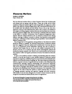
Figure 1: Information gain for the features used to identify DM like.

West tend to overuse like as a DM, as observed in Section 5.3 above. As stated there, a majority of graduate students under 30 came from the US West, therefore it is not possible to single out which of the three features correlates with DM-like overuse. 8.4. Dialogue acts Experiments with the dialogue-act feature used individually, or in conjunction with type, showed that this feature was not useful for DM identification, regardless of the exact representation of the dialogue act labels. Scores did not improve with respect to the baseline when this feature was added to type, and they did not decrease significantly when this feature was removed from the entire set – for like, well, or both items. For instance, the overall best score of κ = 0.783 ± 0.016 (obtained with a Bayesian network) decreased to κ = 0.780 ± 0.016 when the dialogue-act feature was removed, a difference that is not significant at the 95% level. This result is not surprising, as DM well may equally well introduce questions, commands or statements, while the scope of like is generally not an entire utterance. These two DMs are rather related to the topic structure or to the negotiation of the information context, which do not have a direct impact on dialogue acts, unlike, for instance, the DMs studied by Byron and Heeman (1997) in relation to conversational moves. 8.5. Automatic feature selection Feature selection algorithms compare the merits of features in a more systematic way than above, and can extend and/or confirm our previous insights. Two methods from the Weka toolkit were used. Correlation-based feature subset selection (CFS) constructs the best subset of features for DM identification by searching for features with high predictive power, using best-first search with backtracking, while at the same time minimizing redundancy within the subset. Feature relevance can also be computed independently using either the information gain brought by a feature with respect to the DM/non-DM classification, or by computing the χ2 statistic of the feature with respect to the DM class. As feature rankings were very similar, only results using the information gain are reported below. CFS found the following optimal subset of features: {token, pause-before, initial, word(−1)}. This corroborates three important observations made above: (1) lexical collocations are a key feature, especially the word before the candidate DM; (2) it is important to distinguish between like and well using the type feature; and (3) the pause-before the candidate is informative as well. The score of the best feature subset was quite below the best scores obtained using the Bayesian Network or the C4.5 learner, at CCI = 86.8%, κ = 0.69, r = 0.96, p = 0.86, f = 0.91 – κ is especially lower compared to κ = 0.78 for the best classifiers – though the scores increased when merging the best CFS subsets obtained separately for like and for well (CCI = 88.4%, κ = 0.73, r = 0.97, p = 0.87, f = 0.92). The 15

Figure 2: Information gain for the features used to identify DM well.

lower scores of the optimal subset are probably due to the fact that CFS, unlike C4.5, is not aimed directly at finding an optimal classifier, but only at performing feature analysis. The individual ranking of features can be computed over the entire data set or separately for each type. When computed jointly, the highest scoring feature was the word preceding the candidate, followed at some distance by pause-before, initial, word(+1), and type. The other features obtained much lower scores.5 When computed separately for each type, the ranking was different for like than for well, as shown respectively in Figures 1 and 2. For like, the most informative feature was word(−1), followed at some distance by word(+1) and speaker, and all other ones had much lower information gains. For well, the most informative feature was word(−1), followed closely by a group of five features: pause-before, initial, word(+1), pause-after and final. The high rank of speaker for like but not for well confirms that some people have marked preferences for using like, but none for well. Feature selection can also be used to find the most discriminative lexical collocations, if lexical features are encoded using one positional variable per word, indicating the (closest) position of the word with respect to the candidate DM. We ranked these variables first using CFS subsets, and then individually using information gain. In the best feature subsets, five lexical items concerning only like appeared along with other features: something, things and seems were all preceding non-DM like; that was following non-DM like; and to was following non-DM like or preceding it. When applying CFS on like and well separately, two lexical indicators were found for well: as and very, both preceding non-DM occurrences of well. The individual ranking of lexical features, computed separately for like vs. well, showed that some lexical indicators had information gain scores that were comparable to some of the prosodic/positional and sociolinguistic features. The gains were higher for like than for well, probably because like is syntactically bound more often than well. 9. Conclusions We have studied automatic classifiers trained using machine learning for disambiguating candidate DMs, and we have provided in-depth analyses of their application to two highly ambiguous items, like and well, using a large data set. We now summarize the main findings in terms of performance and of contributions of features, and suggest directions for future work. 5 The information gain values for each feature were: word(−1) 0.5167, pause-before 0.2601, initial 0.2226, word(+1) 0.1947, token 0.1550, speaker 0.0385, pause-after 0.0358, final 0.0250, duration 0.0196, age 0.0126, education 0.0059, country 0.0052, native 0.0026, gender 0.0005.

16

Table 8: Comparison of results for DM identification. ‘HL93’ stands for (Hirschberg and Litman, 1993); ‘SM94’ for (Siegel and McKeown, 1994); ‘L96’ for (Litman, 1996); ‘HA99’ for (Heeman and Allen, 1999); ‘Z02’ for (Zechner, 2002); ‘SDS04’ for (Snover et al., 2004); ‘JCL04’ for (Johnson et al., 2004); and ‘PBZ’ for the present study. ‘C’ stands for correctly classified instances (accuracy), ‘n.c.’ for non-conjunct DMs, ‘LFP’ for lexicalised filled pause, ‘SWBD’ for the Switchboard corpus or a subset of it, and ‘c.v.’ for cross-validation.

Study HL93

DM types 1 (well) 34 34 31 (n.c.) 34 34

Tokens 52 878 878 495 1,027 1,027

L96

34

878

HA99 Z02

31 (n.c.) 34 31 (n.c.) ∼ 30 DMs as LFPs

SDS04 JCL04 PBZ

DMs as LFPs 8 DMs as LFPs 2 (like, well)

495 878 495 8,278 DMs 5,787 DMs 2,355 DMs SWBD SWBD 8,655

1 (like)

4,519

Model and/or features intonational hand-coded intonational hand-coded punctuation intonational hand-coded baseline decision tree; punctuation decision tree built by a genetic algorithm; punctuation, lexical features cgrendel or C4.5 decision trees; prosodic and textual features same prosodic phrase same language model with POS POS tagger with lexical features same model on meeting data rule-based model; lexical features, POS manually defined lexical indicators C4.5 decision trees; lexical, temporal and sociolinguistic features same

1 (well)

4,136

same

SM94

Results C = 98.1% C = 75.4%, κ = .52 C = 80.1%, κ = .54 C = 85.3%, κ = .69 C = 79.16% C = 79.20% (58-fold c.v.) C = 83.1% ± 3.4% (10-fold c.v.) C = 83.4% ± 4.1% C = 85.5% ± 3.4% C = 87.4% ± 3.3% C = 93.57% DMs f = .93 f = .30 C = 81.9% DMs C = 81% DMs C = 90.5% ± .6% κ = .78 ± .02 (10-fold c.v.) C = 84.5% ± 1.0% κ = .69 ± .02 C = 97.5% ± .5% κ = .88 ± .02

9.1. DM identification performance The best scores obtained for like and well were CCI = 90%, κ = 0.78, r = 0.96, p = 0.90, and f = 0.93. The confidence intervals at the 95% level were of about ±0.02 for κ and generally lower than ±0.01 for the other scores, as computed with the ten-fold cross-validation procedure. The search for the best meta-parameters of the C4.5 learner and of the lexical features were performed however over the entire data. Therefore, the resulting optimal classifiers should be additionally tested on previously unseen data, when a new data set annotated for DMs becomes available, in order to confirm performance. Another solution would be to use nested cross-validation to estimate the confidence intervals after meta-parameter choice, but this would seriously decrease the amount of data available for each subfold. The best scores were reached by a Bayesian network classifier, but decision trees trained with C4.5, or SVMs, did not score significantly lower. The best scores were considerably higher than those of uninformed baseline classifiers, and still significantly above more informed baselines. For instance, a type-specific majority classifier performed better than the majority classifier that treated all candidates as DMs. Simple classifiers such as the one using only the type and word(−1) features performed above baseline too, but were significantly outperformed by the best classifiers. The best scores were higher for well than for like (98% vs. 85% CCIs) and significantly above type-specific baselines. The best scores were comparable to the inter-annotator agreement values, which reached κ = 0.74 for the best experimental conditions with transcripts and audio recordings. Automatic classifiers have thus reached the highest meaningful performance on the present data set, proving that the set of features was sufficient for that performance. To improve scores in a meaningful way, a more reliable annotation is necessary, which could be obtained by using more annotators, with improved training, and adjudicating their decisions. 17

The present scores compare favorably with those of previous studies, as shown in Table 8. Our scores are higher than most previous ones, with the notable exception of those obtained by Heeman and Allen (1999), who used however a different version of the accuracy score, as noted at the end of Section 6. These differences are also related to the intrinsic difficulty of disambiguating each DM type, as illustrated in Litman’s work by the higher scores obtained when conjuncts and, or, and but were removed from the data. In our experiments, the identification of like appeared to be more difficult than that of well, but a more comprehensive scale of ambiguity remains to be drawn. 9.2. Relevant features The most important features for DM identification were lexical collocations, which were learned automatically from the training data. Among these, the word before a candidate DM was the most useful one, especially as it also encoded the utterance-initial character. Scores obtained using only lexical features were within 5% from the best ones. Positional and prosodic/temporal features were significantly less efficient than lexical ones, when used alone, but they still appeared in the best decision trees just below lexical features. The initial and final character of a token were correlated with its class when tokens were classified separately according to their type. The pause-before and pause-after features were even more reliable indicators, as they also subsume positional features, with pauses of about 60 ms around a token tending to characterize DMs (the value was determined automatically). As for the duration of the token, this was almost always irrelevant to its classification. These findings parallel the observation in Section 4.2 that human annotators were more reliable when prosodic information was available in addition to the transcript. The sociolinguistic features were slightly correlated to the use of DM like: the identity of speakers and their education level sometimes helped to predict the class. Dialogue acts information was not helpful for DM identification over the present data. Finally, the type feature was essential: the two types studied here, like and well, were better processed separately than as a unique type, a conclusion that matches the theoretical analyses arguing that DMs are not a homogeneous class. Although some of the features and values generalized to both types, such as pause-before, many of the most relevant features were type specific, in particular the lexical ones. It is therefore not likely that a general purpose DM classifier could ever outperform a type specific one. On the contrary, as the number of ambiguous DM types is quite small (several dozen), it is preferable, from a machine learning point of view, to build type specific classifiers by using sufficient training data for each type. This finding is consistent with Litman’s (1996) observation that cue phrases were better identified individually rather than as a class. However, it is surprising that Litman’s study did not include lexical features, possibly due to the limited size of the training data for each type. Siegel and McKeown (1994) also argued for the utility of distinguishing DM types in decision trees, although their best scores were in fact close to the baseline. 9.3. Future work Future work should focus on the generalization of the features described above to other highly ambiguous DM types, such as conjuncts (and, or, but) or multiword expressions (you know). This will require manual annotation of a large amount of instances for training and testing, and possibly an adaptation of the features. Prosodic features could be refined to include for instance pitch variation, provided this can be detected automatically from audio recordings, in the case of spoken corpora. The results of a POS tagger trained on speech could be used to generalize lexical collocations using the POS labels of the neighbors of candidate DMs, although, as mentioned in Section 5.4, previous studies showed that the improvements were quite small. Given the strong pragmatic function of DMs, it is nevertheless unlikely that low-level features combined using machine learning will ever solve the DM identification problem entirely. The DM role of an item can be confirmed only by a full semantic/pragmatic analysis of an utterance, which is still a remote goal for computational linguistics in domain-independent cases. However, such an analysis also seems to require, in turn, the disambiguation of candidate DMs. It appears thus that DM identification and semantic/pragmatic analysis are a chicken-and-egg problem, and they might best be performed in parallel. This could be achieved by bootstrapping the two processes with low-level features, then propagating information from one process to another. The technique described in this article offers such a set of low-level features for DM identification.

18

Acknowledgments This work was supported by the Swiss National Science Foundation (SNSF) through the NCCR on Interactive Multimodal Information Management (IM2). We would like to thank Elizabeth Shriberg and Dan Jurafsky for, respectively, their help with the ICSI-MR and Switchboard corpora. References Andersen, G., 2000. The role of the pragmatic marker ‘like’ in utterance interpretation. In: Andersen, G., Fretheim, T. (Eds.), Pragmatic Markers and Propositional Attitude. John Benjamins, Amsterdam, pp. 17–38. Andersen, G., 2001. Pragmatic Markers of Sociolinguistic Variation. John Benjamins, Amsterdam. Artstein, R., Poesio, M., 2008. Inter-coder agreement for computational linguistics. Computational Linguistics 34 (4), 555–596. Brennan, S. E., Schober, M. F., 2001. How listeners compensate for disfluencies in spontaneous speech. Journal of Memory and Language 44, 274–296. Byron, D. K., Heeman, P. A., 1997. Discourse marker use in task-oriented spoken dialogues. In: Proceedings of Eurospeech 1997 (5th European Conference on Speech Communication and Technology). Rhodes, pp. 2223–2226. Carletta, J., 1996. Assessing agreement on classification tasks: The kappa statistic. Computational Linguistics 22 (2), 249–254. Core, M. G., Schubert, L. K., 1999. A syntactic framework for speech repairs and other disruptions. In: Proceedings of ACL 1999 (37th Annual Meeting of the Association for Computational Linguistics). College Park, MD, pp. 413–420. de Klerk, V., 2005. Procedural meanings of well in a corpus of Xhosa English. Journal of Pragmatics 37, 1183–1205. Fraser, B., 1990. An approach to discourse markers. Journal of Pragmatics 14, 383–395. Fuller, J. M., 2003. The influence of speaker roles on discourse marker use. Journal of Pragmatics 35 (1), 23–45. Grosz, B. J., Hirschberg, J., 1992. Some intonational characteristics of discourse structure. In: Proceedings of ICSLP 1992 (2nd International Conference on Spoken Language Processing). Banff, AB, pp. 429–432. Heeman, P. A., 1997. Speech repairs, intonational boundaries and discourse markers: Modeling speakers’ utterances in spoken dialog. Ph.D. thesis, University of Rochester, NY. Heeman, P. A., Allen, J. F., 1999. Speech repairs, intonational phrases and discourse markers: Modeling speakers’ utterances in spoken dialogue. Computational Linguistics 25 (4), 1–45. Heeman, P. A., Byron, D. K., Allen, J. F., 1998. Identifying discourse markers in spoken dialog. In: Proceedings of AAAI Spring Symposium on Applying Machine Learning to Discourse Processing. Stanford, CA. Hirschberg, J., Litman, D. J., 1993. Empirical studies on the disambiguation of cue phrases. Computational Linguistics 19 (3), 501–530. Hirschberg, J., Nakatani, C. H., 1996. A prosodic analysis of discourse segments in direction-giving monologues. In: Proceedings of ACL 1995 (34th Annual Meeting of the ACL). Santa Cruz, CA, pp. 286–293. Hovy, E. H., 1995. The multifunctionality of discourse markers. In: Workshop on Discourse Markers. Egmond-aan-Zee, The Netherlands. Janin, A., Ang, J., Bhagat, S., Dhillon, R., Edwards, J., Macias-Guarasa, J., Morgan, N., Peskin, B., Shriberg, E., Stolcke, A., Wooters, C., Wrede, B., 2004. The ICSI Meeting Project: Resources and research. In: ICASSP 2004 Meeting Recognition Workshop. Montreal. Janin, A., Baron, D., Edwards, J. A., Ellis, D., Gelbart, D., Morgan, N., Peskin, B., Pfau, T., Shriberg, E., Stolcke, A., Wooters, C., 2003. The ICSI Meeting Corpus. In: Proceedings of ICASSP 2003 (28th IEEE International Conference on Acoustics, Speech, and Signal Processing). Vol. 4. Hong Kong, pp. 364–367. Johnson, M., Charniak, E., Lease, M., 2004. An improved model for recognizing disfluencies in conversational speech. In: Proceedings of RT-04F (Rich Transcription 2004 Fall Workshop). Palisades, NY. Jones, D., Wolf, F., Gibson, E., Williams, E., Fedorenko, E., Reynolds, D. A., Zissman, M., 2003. Measuring the readability of automatic speechto-text transcripts. In: Proceedings of Eurospeech 2003 (8th European Conference on Speech Communication and Technology). Geneva, pp. 1585–1588. Jucker, A., 1993. The discourse marker ‘well’: A relevance-theoretical account. Journal of Pragmatics 19, 435–452. Lease, M., Johnson, M., 2006. Early deletion of fillers in processing conversational speech. In: Proceedings of HLT-NAACL 2006 (Human Language Technology Conference of the North American Chapter of the Association of Computational Linguistics), Companion Volume: Short Papers. New York, NY, pp. 73–76. Litman, D. J., 1996. Cue phrase classification using machine learning. Journal of Artificial Intelligence Research 5, 53–94. Marcu, D., 2000. The Theory and Practice of Discourse Parsing and Summarization. The MIT Press, Cambridge, MA. Mason, O., 2000. Programming for Corpus Linguistics: How to do Text Analysis in Java. Edinburgh University Press, Edinburgh. Meteer, M., Taylor, A., MacIntyre, R., Iyer, R., February 1995. Revised by Ann Taylor in June 1995. Dysfluency annotation stylebook for the Switchboard corpus. Tech. rep., Linguistic Data Consortium. Passonneau, R. J., Litman, D. J., 1997. Discourse segmentation by human and automated means. Computational Linguistics 23 (1), 103–140. Penning, M., Theune, M., 2007. Cueing the virtual storyteller: Analysis of cue phrase usage in fairy tales. In: Proceedings of ENLG 2007 (11th European Workshop on Natural Language Generation). Schloss Dagstuhl, pp. 159–162. Petukhova, V., Bunt, H., 2009. Towards a multidimensional semantics of discourse markers in spoken dialogue. In: IWCS-8 (8th International Conference on Computational Semantics). Tilburg, pp. 157–168. Pons Border´ıa, S., 2008. Do discourse markers exist? On the treatment of discourse markers in relevance theory. Journal of Pragmatics 40 (8), 1411–1434. Prasad, R., Dinesh, N., Lee, A., Miltsakaki, E., Robaldo, L., Joshi, A., Webber, B., 2008. The Penn Discourse Treebank 2.0. In: Proceedings of LREC 2008 (6th International Conference on Language Resources and Evaluation). Marrakech. Quinlan, J. R., 1993. C4.5: Programs for Machine Learning. Morgan Kaufman, San Francisco, CA.

19

Reichman, R., 1985. Getting Computers to Talk Like You and Me: Discourse Context, Focus, and Semantics. The MIT Press, Cambridge, MA. Romaine, S., Lange, D., 1991. The use of ‘like’ as a marker of reported speech and thought: A case of grammaticalization in process. American Speech 66 (3), 227–79. Samuel, K., 1999. Discourse learning: An investigation of dialogue act tagging using transformation-based learning. Ph.D. thesis, University of Delaware, Department of Computer and Information Sciences. Samy, D., Gonz´alez-Ledesma, A., 2008. Pragmatic annotation of discourse markers in a multilingual parallel corpus (Arabic-Spanish-English). In: Proceedings of LREC 2008 (6th International Conference on Language Resources and Evaluation). Marrakech. Schiffrin, D., 1987. Discourse Markers. Cambridge University Press, Cambridge, UK. Schourup, L. C., 1985. Common Discourse Particles in English Conversations: ‘Like’, ‘Well’, ‘Y’know’. Garland, New York, NY / London, UK. Schourup, L. C., 1999. Discourse markers. Lingua 107, 227–265. Schourup, L. C., 2001. Rethinking ‘well’. Journal of Pragmatics 33, 1025–1060. Shriberg, E., Bates, R., Taylor, P., Stolcke, A., Jurafsky, D., Ries, K., Coccaro, N., Martin, R., Meteer, M., Van Ess-Dykema, C., 1998. Can prosody aid the automatic classification of dialog acts in conversational speech? Language and Speech 41 (3-4), 439–487. Shriberg, E., Dhillon, R., Bhagat, S., Ang, J., Carvey, H., 2004. The ICSI meeting recorder dialog act (MRDA) corpus. In: Proceedings of SIGdial 2004 (5th SIGdial Workshop on Discourse and Dialogue). Cambridge, MA, pp. 97–100. Siegel, E. V., McKeown, K. R., 1994. Emergent linguistic rules from inducing decision trees: Disambiguating discourse clue words. In: Proceedings of AAAI 1994 (12th National Conference on Artificial Intelligence). Seattle, WA, pp. 820–826. Snover, M., Dorr, B., Schwartz, R., 2004. A lexically-driven algorithm for disfluency detection. In: Proceedings of HLT-NAACL 2004 (Human Language Technology Conference of the North American Chapter of the Association for Computational Linguistics). Boston, MA, pp. 157–160. Stolcke, A., Shriberg, E., Bates, R., Ostendorf, M., Hakkani, D., Plauche, M., T¨ur, G., Lu, Y., 1998. Automatic detection of sentence boundaries and disfluencies based on recognized words. In: Proceedings of ICSLP 1998 (5th International Conference on Spoken Language Processing). Sydney. Traugott, E. C., 1995. The role of the development of discourse markers in a theory of grammaticalization. In: XIIth International Conference on Historical Linguistics. Manchester. Verdonik, D., Rojc, M., Stabej, M., 2007. Annotating discourse markers in spontaneous speech corpora on an example for the slovenian language. Language Resources and Evaluation 41 (2), 147–180. Witten, I., Frank, E., 2000. Data Mining: Practical Machine Learning Tools with Java Implementations. Morgan Kaufmann, San Francisco, CA. Zechner, K., 2002. Automatic summarization of open-domain multiparty dialogues in diverse genres. Computational Linguistics 28 (4), 447–485. Zufferey, S., Popescu-Belis, A., 2004. Towards automatic identification of discourse markers in dialogs: The case of ‘like’. In: Proceedings of SIGdial 2004 (5th SIGdial Workshop on Discourse and Dialogue). Cambridge, MA, pp. 63–71.

20