Automatic Inference of Models for Statistical Code Compression Christopher W. Fraser Microsoft Research One Microsoft Way, Redmond, WA 98052 USA
[email protected]
ABSTRACT This paper describes experiments that apply machine learning to compress computer programs, formalizing and automating decisions about instruction encoding that have traditionally been made by humans in a more ad hoc manner. A program accepts a large training set of program material in a conventional compiler intermediate representation (IR) and automatically infers a decision tree that separates IR code into streams that compress much better than the undifferentiated whole. Driving a conventional arithmetic compressor with this model yields code 30% smaller than the previous record for IR code compression, and 24% smaller than an ambitious optimizing compiler feeding an ambitious general-purpose data compressor.
Keywords Abstract machines, code compaction, code compression, compiler intermediate languages and representations, data compression, decision trees, machine learning, statistical models, virtual machines.
MOTIVATION Compressing code can reduce important bottlenecks in current computer systems, including: •
Network transmission time, especially for downloads over conventional telephone lines, but faster networks may benefit as well.
•
Load time from disk during application start-up.
•
ROM for embedded computers.
For example, most software delivered via the Internet is already compressed; OS-level disk compression implicitly reduces load time; and handheld computers routinely compress the applications in ROM. For many such scenarios, memory or transmission time is much scarcer than processor cycles, and the "cost" of any
Copyright © 1999 by the Association for Computing Machinery, Inc. Permission to make digital or hard copies of part or all of this work for personal or classroom use is granted without fee provided that copies are not made or distributed for profit or commercial advantage and that copies bear this notice and the full citation on the first page. Copyrights for components of this work owned by others than ACM must be honored. Abstracting with credit is permitted. To copy otherwise, to republish, to post on servers, or to redistribute to lists, requires prior specific permission and/or a fee. Request permissions from Publications Dept, ACM Inc., fax +1 (212) 869-0481, or
[email protected].
reasonable incremental decompression can be negative. That is, saving even a few percent in size frees up more than enough resources to implement the decompressor. Some scenarios — particularly those that require direct interpretation of the compressed code — do not fit these requirements, but many do. This paper's principal focus is not the details of the actual encoding but rather the more basic problem of statistical models that reduce entropy, because such models lead directly to a variety of compact encodings. The entropy of English text, for example, has been studied for decades [Shannon] with results including a good understanding of the limits on text compression. Now that compiled code accounts for so much of the data transmitted between and stored on many computer systems, its entropy and limits merit similar study.1
BACKGROUND: DATA COMPRESSION Current general-purpose data compressors follow a statistical modeler with a coder [Bell, Cleary, and Witten]. LZ coders [Lempel and Ziv, Ziv and Lempel] can be modeled by such systems, but the converse is not true, so it suffices to focus on statistical modelers. As the input is compressed or decompressed, the modeler tracks some context and identifies a probability distribution that the coder (e.g., an arithmetic coder) uses to encode the next token. For example, when compressing English text, the letter Q is often followed by the letter U, so a good modeler responds to a Q by switching to a distribution that assigns a high probability to a U and thus encodes it in less space. Markov models use the last N tokens to help predict and compress the next token. That is, for an alphabet A, an order-N Markov model uses up to |A|N probability distributions, one for each combination of the last N tokens. PPM (Prediction by Partial Matching) modelers blend or switch on the fly between several Markov models, preferring more history when the recent context has been seen often and backing off to use less history when it has less experience with the current context. Whatever the method, the objective is to build a model that assigns a non-zero probability to every valid message, and high probabilities to messages that resemble those in some 1
The subject of this research is code compression, so it is assumed throughout this paper that the data segment — that is, initialized data and out-of-line literals — are handled separately, perhaps by a general-purpose data compressor.
representative training set S. The higher the probability assigned to a message M=m1 m2 … mN, the shorter its minimum codelength, which is expressed by its entropy and equals −N⋅Σ P(mi) ⋅log2(P(mi)) where P(x) denotes the model’s estimate of the probability of the symbol x. Typically P(x) is approximated using frequencies from the training set S organized within the model's structure. For example, an order-0 Markov model estimates P(x) with freq(x)/|S|, where freq(x) denotes the number of times that x appears in the training set S.
For example, a typical run from the measurements below includes a subsample with entropy of 91 bits. The decision-tree learning algorithm discovers, however, that splitting the sample by comparing one of the predictors with one of its values yields subsamples with entropies 65 bits and zero bits (because the latter partition includes only one distinct value). No other predictor yields a more promising partition for this sample, so the algorithm commits to this particular comparison and recursively tries the smaller partitions, though the second bottoms out immediately.
DECISION TREES
The research presented below has used two different programs to infer decision trees: a straightforward implementation of the textbook algorithm above [Langley] partly tailored to code compression, and a more statistically sophisticated, generalpurpose system [Chickering, Heckerman, and Meek], which produces better decision trees and can produce “decision dags,” which allow similar contexts or partitions to share frequency distributions. The general-purpose system produced the measurements presented below, but the special-purpose implementation has been useful for simple experiments and may prove necessary to compress larger inputs.
One way to identify good contexts is to propose a large number of predictors that might be worth tracking and then automatically inferring a decision tree that sifts through them. For example, consider the problem of compressing a postfix compiler IR code. Predictors might include the stack height, the last few operators and a bit that records if the next input is an opcode or literal data. An inferred decision tree might be:
This inference process is expensive but not prohibitive. This research typically used 20-50 predictors drawn from a space of about 100 values and generated decision trees in 10-20 minutes on a 300MHz P2 with 256MB of RAM. These costs are currently too high for routine compression, but not for the definition of compressed instruction set nor for compressing code for delivery via constrained media such as ROM or slow networks.
The partition of the compression problem into modeling plus coding is a programming abstraction: the modeler knows nothing about the encoding, and the coder's only knowledge of the input comes from the probability distributions. Coders are usefully left to experts in data compression, but statistical models can benefit from experience with possible sources of redundancy in the data being compressed, here compiler IR code.
BACKGROUND: MACHINE LEARNING OF
if height = 0 then use distribution1 else if inLiteral then use distribution2 else use distribution3 In this example, one predictor (the last operator) has not been used, and the stack height has been found more useful than the literal indicator. The input to algorithms that infer such decision trees is a training set S (in the application at hand, a large set of compiler IR code) and a set of predictors associated with each token in S (e.g., the last few symbols, the stack height, the types of the elements on the stack). The output is a decision tree that tests some of the predictors and, at each leaf, yields a probability distribution that suits the context defined by those tests. The standard algorithm operates as follows: •
For each predictor P, and for each value VP assumed by P in the training set S, perform a trial partition of the sample into two parts: those for which P equals VP, and those for which P equals something else. Compute the entropy in bits of each part and the sum of the two entropies. Let Emin denote the minimal such sum for all values of P and VP.
•
If Emin is less than entropy(S), then add to the decision tree a node that compares the predictor and value associated with Emin. Partition the sample based on this comparison and recursively infer a decision tree for each half of the partition.
•
IR PREDICTORS IR code is full of material that can help predict what’s coming next. For example, after a comparison instruction, conditional branches are far more common than anything else. Otherwise, why would the programmer and compiler place the comparison there? Compressors can exploit this fact by using an especially short opcode for the branch in this special context, or by compressing with an equivalent probability distribution. Opcodes can also help predict elements of the operand stream. For example, programs are much more likely to add 1 than 3, and a load into register R tends to increase the probability that the next instruction or two reads R. Thus the probability distribution of opcodes is different after comparisons, and likewise the probability distribution of operands is different after adds and loads. The problem at hand is identifying a set of distributions that compresses typical programs efficiently. The approach presented here proposes a large number of potentially useful predictors and applies a machine-learning algorithm to identify the predictors and contexts that prove useful in a large training set. This research uses three kinds of predictors: •
The last few (typically 10-20) tokens seen. Such “Markov” predictors capture idioms such as the compare-branch and add-1 patterns above. The predictors give the modeler access to the information tracked by both Markov and PPM modelers.
•
Computed predictors such as the stack height (the IR is postfix) and datatype — integer, real, or pointer — of the top few stack elements. Computed predictors encode domain-
Otherwise, return a decision-tree leaf, namely the probability distribution of the sample S.
This process converges because eventually the decision tree forms sub-samples with only one distinct value, for which the entropy is zero.
specific knowledge that is not explicitly available to generalpurpose compressors. •
Reduced predictors, which project a set of related predictors (e.g., the opcodes EQ, NE, GT, GE, LT, LE) onto a singleton (e.g., REL), which naturally occurs more often and thus allows the machine-learning phase to arrive at useful frequency distributions more quickly. The reduced predictors do not replace the original, unreduced predictors; rather, both the reduced and unreduced predictors are made available to the machine-learning algorithm, which is free to choose whichever works best in each context. Reduced predictors, like computed predictors, also add domain-specific knowledge.
In principle, a good decision-tree generator and data compressor should be able to do without computed and reduced predictors, given enough training data, but the extra heuristic data is easy to provide and helps the system find a useful decision tree much sooner. Predictors vary widely in expected value: •
•
•
When the stack is empty, binary operators are syntactically invalid, so their probabilities are zero, and the coder should waste no coding bits on them. Indeed, in this context, there is no need to code for any but null-ary or leaf opcodes. When the top of the stack holds an address, an indirection opcode typically has a higher than average probability, and floating-point opcodes, for example, are invalid. When the previous opcodes leave integers on top of the stack, the probability distribution is surely skewed somewhat — for example, ADD is typically more probable than DIV — but it is less skewed and thus less profitable than the two partitions discussed just above.
THE RAW INPUT For the measurements below, lcc was adapted [Fraser and Hanson] to emit a linearized, postfix rendition of its IR code stream, which roughly resembles code for a stack VM. For example, it transforms the C statement i=j into the first column below: ADDRGP i
push the address of global j
ADDRGP j
push the address of global i
INDIRI
pop an address and push the int at that address
ASGNI
pop an address and int and store the latter at the former
opcodes to 56. Given enough data and time, the decision-tree inference algorithm should, of course, be able to replicate this trick automatically, but this transformation was an easy way to save time. Ignoring the literals — for example, the addresses i and j — for the time being, the next step generates the predictors that are available just before each of the opcodes at hand, e.g., stack tyTop prev prev2 … height ADDRG 0 None None None … ADDRG 1 addr ADDRG None … INDIRI 1 addr ADDRG ADDRG … ASGNI 2 int INDIRI ADDRG … The result is a large, two-dimensional table. It has one row for each token that lcc emits. Its first column holds those tokens, and the remaining columns hold the predictors available (i.e., the context or state) at that site, which is just before that predictee was seen. The predictors comprise the state that is available to help predict the predictee. They are the raw material for the contexts or partitions that are automatically inferred and represented as a decision tree. predictee
The instruction stream also includes material other than operators, namely: •
Immediate constants.
•
Global identifiers.
•
Offsets of locals and formals.
•
Label definitions and references.
All of these streams are folded into the opcode stream, in order to make them available as both predictors and predictees. Modest preprocessing is performed to make them more useful in these roles and to avoid gratuitous bloat: •
Immediate constants are represented by the corresponding string of decimal digits. For example, the IR that pushes 14 onto the stack is represented with three bytes: the lcc IR opcode CNST, the ASCII digit 1, and the ASCII digit 4. A more conventional fixed-width representation for constants did not compress as well, presumably because the extra zeroes diluted the more useful predictors. This representation effectively adds eleven “opcodes” — one for each of the ten decimal digits, plus one for the minus sign — to the 56 described above.
•
References to globals are separated by segment (code versus data) and passed through a MTF coder3. The resulting integers are coded just like the constants above, and the escaped string names are moved to a separate string table, which is compressed by a conventional text compressor.
3
A move-to-front or MTF coder maintains a buffer, which starts empty. The coder then repeatedly reads the next input token X. If X is in the buffer, then the coder emits the number of the position in which X appears and moves X to the head of the buffer. Otherwise, the coder emits an escape code followed by X and inserts X at the head of the buffer.
Next, all trivially inferrable IR data-types and sizes — for example, lcc's distinct integer and real addition opcodes are gratuitous when the stack-type predictors uniquely identify the opcode's type qualifier — are removed, which reduced2 lcc’s 119 2
Reducing the operator set is not to be confused with reduced predictors. Reducing the operator set effects predictees and can discard only information that can be reconstructed from context. Reducing predictors effects only predictors and can discard any information, though the machine-learning system is likely to find little use for predictors that discard too much (or, for that matter, too little) information.
•
References to locals and formals are also MTF-coded, but their respective MTF buffers are naturally cleared between procedures.
•
Labels are renumbered consecutively — thus obviating the need to include a label number with each label definition — and label references are delta-coded (i.e., made relative to the number implicit in the last label definition).
The three cases immediately above add five opcodes — one to flag the head of a new procedure and one for each of the four MTF escape codes — which brings the number of “opcodes” to 72. That is, the lcc back end employed in this research emits output that uses an alphabet of 72 different symbols. The methods above, of course, do some compression themselves, but the literal and constant data have to be represented somehow, and it is arguable that the encodings above are natural for the material in question: delta-coding is the obvious choice for label numbers that grow steadily during compilation, and MTF-coding is the natural expression in this context of the well-known principle of temporal locality.
EXPERIMENTAL MEASUREMENTS Table 1 compares the method of this paper with several other compressors. The compressee is the GNU C compiler, gcc. That is, the code being compressed is the IR code generated by lcc for gcc. The IR code is represented as described in the previous section. Gzip [Gailly and Adler] is version 1.2.4 of the currently ubiquitous GNU compression utility, and Bzip2 [Seward] is a Burrows-Wheeler compressor [Burrows and Wheeler]. Azip is an arithmetic compressor that uses a single frequency distribution computed during a pre-scan of the input; that is, it uses a memoryless or order-zero Markov model. Bytes Compressor 1,015,495 uncompressed
Ideally, Table 1 would also include comparisons with Franz’s “slim binaries” for Oberon [Franz; Franz and Kistler] and the emerging Java class-file compressors [Horspool and Corless], but these methods require different source languages, so no direct comparisons are possible. Table 2 compares the compression of lcc’s IR and x86 code. The IR code compresses considerably better. It starts off only about 10% smaller, but this margin widens with all of the tested compressors. lcc’s IR code
lcc’s x86 code
Compressor
1,015,495
1,122,991
589,393
786,096
azip
287,260
370,257
gzip
249,165
304,922
bzip2
195,236
NA
uncompressed
this research
Table 2. Compressing IR versus machine code. When the goal of compression is the efficient delivery of an executable via some bottleneck, the measurements in Table 2 suggest that it can be effective to transmit IR code and generate code on the receiver, although the methods described in this paper are being adapted to compress conventional executables, so this trade-off might change. Table 3 shows the effect of vigorous optimization. It parallels Table 2 but with x86 code from the Microsoft Visual C/C++ compiler, which was configured to minimize space usage (namely, option “/O1”). lcc’s IR code
MSVC /O1
Compressor
1,015,495
623,581
uncompressed
589,393
447,563
azip
287,260
299,430
gzip
589,393 azip
249,165
255,440
bzip2
295,588 gzip
195,236
NA
287,260 “wire-code" [Ernst] 249,165 bzip2 195,236 this research
Table 1. Comparison of IR code compressors. The compressed string names for the global symbols add another 6,554 bytes, which is necessary for a fair comparison with the "wire code" row in Table 1 but not for comparisons with any other values in Tables 1-3, which count only the code segment and do not include symbolic information. The present method’s result is 30% smaller than the “wire code” in Table 1 [Ernst et al], which appears to be the previous record for the compression of comparable data. The cited paper starts with a larger encoding of the lcc IR, namely 1,381,304 bytes uncompressed and 380,351 bytes after gzip. It thus seems likely that the wire code would benefit from starting with the new representation above, particularly its representation of literal and constant data, but it is not possible to quantify this speculation without repeating the work on the wire code.
this research
Table 3. Compressing IR vs. optimized machine code. Despite the handicap of a much larger starting point, aggressive IR compression yields a result 24% smaller than aggressively optimized (CISC) machine code fed to the best of the generalpurpose data compressors in this trial. The decision dag generated for compressing gcc has 854 nodes but only 66 leaves. That is, the input is divided into 855 streams but many are similar enough that they compress well with only 66 distinct frequency distributions. A straightforward representation of the decision dag compresses to 9022 bytes and could be included with the compressed data, but the machine-learning software takes precautions to avoid overfitting the decision dag to its input, so the dag should be useful for many compressees, and thus many applications would amortize the cost of transmitting or storing the dag over many uses.
RELATED WORK The literature on code compression is large [van de Wiel], though much of it concerns methods that either require no decompression
(e.g., synthesizing procedures from replicated codes) or can be decompressed in hardware, which currently requires techniques that are simpler than this one, so a full review of the literature would be neither germane nor fair.
[2] M. Burrows and D. J. Wheeler. A block-sorting lossless data
Closer in spirit to the present research are compressors that work on compiler IR or VM code [Ernst et al; Franz; Franz and Kistler; Fraser and Proebsting; Horspool and Corliss; Proebsting]. In general, these compressors divide their input into manually identified streams or exploit repeated pairs or trees or both.
approach to learning Bayesian networks with local structure. Proceedings of the Thirteenth Conference on Uncertainty in Artificial Intelligence, Morgan Kaufman, 8/97.
The present method was designed to subsume these two methods with a single, more general method. The leaves of the decision tree partition the input into streams of similar data, but the partitioning is now automatic, and the streams are far finer than is practical with manual identification. The predictors reach back far enough to catch all but the largest juxtapositions, but the method is not obliged to use all predictors and can include patterns with “holes” in them. The system also has access to computed and reduced predictors that have no clear analogues in the previous work, and it is easily extended by adding new predictors. Indeed, this research can be regarded as the next step in a progression toward increasing automation of code compression: •
•
•
compression algorithm. Digital SRC research report 124, 5/10/94.
[3] D. Chickering, D. Heckerman, and C. Meek. A Bayesian
[4] Jens Ernst, William Evans, Christopher W. Fraser, Steven Lucco, and Todd A. Proebsting. Code compression. PLDI’97:358-365, 6/97. [5] M. Franz and T. Kistler. Slim binaries. TR 96-24, Dept of Information and Computer Science, University of California, Irvine, 6/96. [6] M. Franz. Adaptive compression of syntax trees and iterative dynamic code optimization: Two basic technologies for mobile-object systems. TR 97-04, Dept of Information and Computer Science, University of California, Irvine, 2/97. [7] Christopher W. Fraser and David R. Hanson. A Retargetable C Compiler: Design and Implementation. Addison Wesley Longman, 1995.
Much early work on statistical modeling of program code was done as part of a manual instruction set design. The designers picked some or all of their compressed instruction sets by eyeballing opcode frequencies. They identified the heuristics or patterns to use — for example, all pairs — and then they also identified the pairs that looked best [Sweet].
[8] Christopher W. Fraser and Todd A. Proebsting. Custom Instruction Sets For Code Compression. Unpublished manuscript, http://research.microsoft.com/~toddpro/papers/ pldi2.ps, 10/95.
More recent efforts reduce the manual component by having a program identify the best patterns (e.g., opcode-opcode and opcode-literal pairs in BRISC [Ernst et al] or the opcode trees in the previous record-holding "wire code" [Ernst et al]). This automation helps, but it became clear that different heuristics suit different contexts: sometimes pairs are best, sometimes triples, sometimes using a destination register to predict a subsequent source register, etc.
[10] Jean-Loup Gailly and Mark Adler. The gzip home page. http://w3.gzip.org. 1/21/99.
This paper reduces manual effort still further. The human identifies not the heuristics or patterns, but rather identifies a set of heuristics that might help in some contexts. The software then selects the combinations that yield good results.
[13] A. Lempel and J. Ziv. On the complexity of finite sequences. IEEE Transactions on Information Theory 22(1):75-81, 1/76.
ACKNOWLEDGMENTS Max Chickering, David Heckerman, David Hovel, and Chris Meeks supplied the general-purpose decision-dag generator and were generous with their time answering my questions and adapting their code. The author is also grateful for suggestions and support from Suzanne Bunton, Will Evans, Bill Gates, Dave Hanson, Steve Lucco, John Miller, Nathan Myhrvold, Todd Proebsting, and Rick Rashid.
REFERENCES [1] Timothy C. Bell, John G. Cleary, and Ian H. Witten. Text Compression. Prentice Hall, 1990.
[9] Free Software Foundation. GCC – The GNU C Compiler. http://www.gnu.org/software/gcc, 8/13/98.
[11] Pat Langley. Elements of Machine Learning. Morgan Kaufmann, 1996. [12] R. Nigel Horspool and Jason Corless. Tailored compression of Java class files. Software — Practice and Experience 28(12):1253-1268, 10/98.
[14] Todd A. Proebsting. Optimizing an ANSI C interpreter with superoperators. POPL’95: 322-332, 1/95. [15] Julian Seward. The bzip2 and libbzip2 home page. http://www.muraroa.demon.co.uk, 2/11/99. [16] C. E. Shannon. Prediction and entropy of printed English. Bell System Technical Journal 30:50-64, 1/51. [17] Richard E. Sweet. Empirical analysis of the Mesa instruction set. ASPLOS’82:158-166. 3/82. [18] Rik van de Wiel. Code compaction bibliography. http://www.win.tue.nl/cs/pa/rikvdw/bibl.html, 2/3/99. [19] Tong Lai Yu. Data compression for PC software distribution. Software-Practice & Experience 26(11):1181-1195, 11/96. [20] J. Ziv and A. Lempel. Compression of individual sequences via variable-rate coding. IEEE Transactions on Information Theory 24(5):530-536, 9/78.