Automatic method to monitor floating macroalgae ... - OSA Publishing

Vol. 26, No. 21 | 15 Oct 2018 | OPTICS EXPRESS 26810

Automatic method to monitor floating macroalgae blooms based on multilayer perceptron: case study of Yellow Sea using GOCI images ZHONGFENG QIU,1,* ZHAOXIN LI,1 MUHAMMAD BILAL,1 SHENGQIANG WANG,1 DEYONG SUN,1 AND YANLONG CHEN2 1School

of Marine Sciences, Nanjing University of Information Science & Technology, Nanjing 210044, China 2National Marine Environmental Monitoring Center, Dalian 116023, China *[email protected]

Abstract: Timely and accurate information about floating macroalgae blooms (MAB), including their distribution, movement, and duration, is crucial in order for local government and residents to grasp the whole picture, and then plan effectively to restrain economic damage. Plenty of threshold-based index methods have been developed to detect surface algae pixels in various ocean color data with different manners; however, these methods cannot be used for every satellite sensor because of the spectral band configuration. Also, these traditional methods generally require other reliable indicators, and even visual inspection, in order to achieve an acceptable mapping of MAB that appears under diverse environmental conditions (cloud, aerosol, and sun glint). To overcome these drawbacks, a machine learning algorithm named Multi-Layer Perceptron (MLP) was used in this paper to establish a novel automatic method to monitor MAB continuously in the Yellow Sea, using Geostationary Ocean Color Imager (GOCI) imagery. The method consists of two MLP models, which consider both spectral and spatial features of Rayleigh-corrected reflectance (Rrc) maps. Accuracy assessment and performance comparison showed that the proposed method has the capability to provide prediction maps of MAB with high accuracy (F1-score approaching 90% or more), and with more robustness than the traditional methods. Most importantly, the model is practically adaptable for other ocean color instruments. This allows customized models to be built and used for monitoring MAB in any regional areas. With the development of machine learning models, long-term mapping of MAB in global ocean is conducive to promoting the associated studies. © 2018 Optical Society of America under the terms of the OSA Open Access Publishing Agreement

1. Introduction Events of rapid accumulation in the population of floating algae, commonly called blooms, have been reported in global freshwater and ocean systems for decades [1–4]. Various types of floating algae bloom have been observed worldwide, such as the toxic Karenia brevis (responsible for ‘red tides’) for the Florida shelf and Gulf of Mexico, the macroalgae including greenish Ulva prolifera (known as ‘green tides’) and brownish Sargassum commonly for both Asian and American coastal regions [5–8]. These massive algae blooms can significantly devastate the local ecological environment by causing the degradation of water quality and beaching events, and then have an adverse impact on human health, tourism, fishery industries and economies [9]. In China, the recurrent floating macroalgae blooms (MAB) at different scales in coastal waters of the East China Sea (ECS) and the Yellow Sea (YS) were documented dating back to 2000 [10,11], which is a big challenge for local government to reduce the subsequent damage. For example, the unexpected outbreak of U. prolifera appeared in the YS during the summer #342823 Journal © 2018

https://doi.org/10.1364/OE.26.026810 Received 20 Aug 2018; revised 23 Sep 2018; accepted 24 Sep 2018; published 1 Oct 2018

Vol. 26, No. 21 | 15 Oct 2018 | OPTICS EXPRESS 26811

of 2008, which was reported as an unprecedented event for its astonishing spatial scale, spent over $100 million for the cleanup to guarantee the holding of Olympic sailing games [12,13]. This incident promoted numerous follow-on work on the origin, evolvement, and duration of MAB. It has been argued that the abnormal biomass accumulation of U. prolifera in the YS was attributed to the unsanitary harvesting operations of Porphyra yezoensis cultivated along the coast of Jiangsu province [14–16]. Whereas, a recent study suggested that the progressive eutrophication of coastal waters in the YS may be primarily responsible for the occurrence of U. prolifera blooms [17]. For the purpose to further understand the interdisciplinary mechanism about what triggers algae blooms and how they may expand, timely and accurate information is requisite. Ocean color satellite data have the advantage of providing frequent and synoptic observations over inland and oceanic waters, playing a crucial role in retrieving historical algae activities and monitoring upcoming bloom events in near-real time. To date, multisource ocean color imagery and algorithms have been dedicated to remotely detect algae blooms in different countries. For instance, Maximum Chlorophyll Index (MCI) was first proposed by Gower et al. [18] specially for Medium Resolution Imaging Spectrometer (MERIS) imagery, facilitating the systematic exploration of Sargassum distribution patterns in the Gulf of Mexico and North Atlantic Ocean between 2002 and 2011 [2,19–21]. Besides, Moderate Resolution Imaging Spectroradiometer (MODIS) imagery was also thought to be a desirable source for mapping floating materials in various aquatic systems [22–24]. In 2008, Hu et al. used the MODIS-derived map of Normalized Difference Vegetation Index (NDVI) with a 250-m resolution to identify U. prolifera features in the YS successfully [13]. To improve the stability of algae detecting algorithm, Hu et al. developed Floating Algae Index (FAI) with a concept of baseline subtraction [25], which is robust to variable atmospheric effects. Similar index named Virtual-Baseline Floating macroAlgae Height (VB-FAH) was introduced for HJ-1A and HJ-1B due to the absence of Short-Wave Infrared (SWIR) waveband, revealing the bloom history in the YS and ECS during 1995–2006 and 2009–2014, respectively [26]. For Geostationary Ocean Color Imager (GOCI) instrument, Son et al. developed the Index of floating Green Algae for GOCI (IGAG) that can enhance the subtle algae signals in complex water areas compared to NDVI [27], so as to exploit the potential value of GOCI imagery in tracking MAB dynamically in the YS, ECS and coastal zones in Japan. Indeed, aforementioned methods can effectively diagnose floating algae slicks (or patches) in regional areas through a threshold predetermined by a veteran person. But, in fact, these threshold-based methods may be invalid when the image is contaminated by clouds, aerosol and sun glint, making the operational use is not straightforward. There have been several attempts to enable robust isolation of algae pixels. A feasible principle is to remove background water signal from the interested scene so that the distribution of local algae index can be normalized. Once the background values of an algae index image are highly uniform, it will be possible to isolate floating algae pixels using a global-scope threshold. The idea was implemented in literature published by Shi and Wang [28], where Normalized Difference Algae Index (NDAI) was introduced, and NDAI value of a given algae pixel will subtract the averaged value of surrounding non-algae pixels to refine the NDAI scene. Inspired by their work, Garcia et al. proposed a semiautomatic algorithm, termed Scaled Algae Index (SAI), that scales NDVI or FAI imagery by subtracting median local ocean value and then segments algae pixels by a scene-wide exclusion method [29]. On the other side, Wang and Hu established a systematic framework to generate Sargassum distribution and coverage maps from Visible Infrared Imager Radiometer Suite (VIIRS) and MODIS Alternative FAI (AFAI) images in conjunction with other indicators to beforehand mask cloud, cloud shadow, sun glint and land-adjacent pixels [26,30]. The method yielded the long-term statistics of Sargassum area coverage from 2000 to 2016 over the Central West Atlantic satisfactorily using MODIS and VIIRS data. Moreover, Qi et al. reported alike research about long-term

Vol. 26, No. 21 | 15 Oct 2018 | OPTICS EXPRESS 26812

trends of U. prolifera bloom in the western YS from 2007 to 2015 using a similar approach [31]. Although there have been several alternative methods recommended, they may not be practically applied to different satellite data, and their feasibility for the complicated largescale environment is not thoroughly acknowledged. In short, an operating system to monitor MAB fully automatically is still rarely investigated. Therefore, the objective of this paper is to establish a robust, fully automatic method that technically practicable for various ocean color data to monitor MAB in the long term. Machine learning approach was employed to serve this purpose, which has become a research hotspot in image classification especially for terrestrial materials [32-34], and was used in a pioneering study to predict red tide pixels for the West Florida Shelf [35]. Here, a case study about using machine learning models based on GOCI images was presented to detect MAB happened in the YS. 2. Data and methods 2.1 Study area The study area, the YS, is bounded by 30.5°N–38°N and 118.5°E–125°E (Fig. 1(a)), a turbid marginal sea of the western Pacific Ocean mainly due to the sediments supplied by the Yangtze River and the Yellow River [36]. The Subei Shoal, well-known as the venue of early aggregates of U. prolifera that mostly occur in May every recent year [37], is dominated by tidal forcing that driving northward residual current during spring tide [38,39]. Under the actions of the wind- and tide-driven surface current, small pieces of U. prolifera that discarded in mudflat and washed into water when P. yezoensis is harvested in the late April, can be advected to the north-east and eventually induce a massive bloom with favorable water conditions on June [10,15]. Besides greenish U. prolifera, the YS is also known to be abundant in Sargassum that commonly transported from the ECS to the north [40]. So, the research of monitoring MAB in this area is highly necessary.

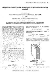
Fig. 1. (a) GOCI AFAI image acquired on 26 May 2017 (03:16:43 GMT) showing floating macroalgae blooms and clouds outlined in the white dashed ellipses over the YS. Dark purple color indicates relatively turbid water, especially at the Subei Shoal. (b) GOCI measured mean Rayleigh-corrected reflectance (Rrc, unitless) spectra of macroalgae, cloud, turbid and clear water pixels collected using ENVI ROI tool with respective standard deviation.

Vol. 26, No. 21 | 15 Oct 2018 | OPTICS EXPRESS 26813

2.2 Satellite data and pre-processing GOCI Level-1B data during May to August of 2016 to 2017 (eight images per day from 00:15 to 07:45 GMT with 500-m spatial resolution) were obtained from the Korea Ocean Satellite Center (KOSC, http://kosc.kiost.ac.kr/). The GOCI standard atmospheric correction, which is based on the algorithm of the Sea-viewing Wide Field-of-view Sensor (SeaWiFS) [41], was processed to generate Rayleigh-corrected reflectance (Rrc, unitless) using the GOCI Data Processing System (GDPS, version 1.3) [42,43]. In brief, the Rrc data at eight spectral bands of 412, 443, 490, 555, 660, 680, 745 and 865 nm contained in Level-2C product was derived as the following equation: Rrc,λ = π LCorr TOA,λ / ( F0,λ cos θ s ) − Rr,λ

(1)

where LCorr TOA,λ is the vicarious calibrated top-of-atmosphere radiance at λ band after gaseous absorption and whitecap correction, F0,λ is the extraterrestrial solar irradiance adjusted according to image acquisition date, θs is the solar zenith angle, and Rr,λ is the Rayleigh reflectance. Then, all Rrc data were mapped into equidistant geographic coordinates with 0.005° spatial resolution of the entire study region. Pseudo color images were composed for visual inspection using Rrc at 865, 660, 555 nm as R, G, B channels, respectively. Moreover, Landsat 8 Operational Land Imager (L8/OLI) images that captured floating macroalgae blooms over the study area during 2016 and 2017 were download from the United States Geological Survey (USGS, https://earthexplorer.usgs.gov/) aiming at cross sensor comparison. The downloaded Level-1 data has a spatial resolution of 30m at eight spectral bands and a 16-day repeat cycle. A similar atmospheric correction was performed using ACOLITE processor [44–46] (https://odnature.naturalsciences.be/remsem/acoliteforum/). 2.3 Scientific indexes For better understanding the spectral characteristics of different targets in Rrc images over the YS, the most concerned classes of macroalgae, cloud, turbid and clear water pixels were selected from several scenes using ENVI Region of Interest (ROI) tool designed to extract image information by visual inspection or a specified pixel value threshold. The corresponding Rrc spectra of the respective class were obtained and showed in Fig. 1(b) in terms of spectral mean and standard deviation. Furthermore, AFAI and NDVI are introduced to delineate macroalgae and water (turbid or clear) pixels [26,47]. Particularly, U. prolifera and Sargassum can both result in high AFAI values (Fig. 1(a)), but distinguishing these two types of macroalgae may require hyperspectral data [48] and this is beyond the scope of this paper; NDVI defined here is actually equivalent to NDAI [28], still, we term it as the former for simplicity. AFAI and NDVI can be derived for each pixel as below:

AFAI=Rrc,NIR − [ Rrc,RED +( Rrc,LNIR − Rrc,RED )(λ NIR − λ RED ) / (λ LNIR − λ RED )]

(2)

NDVI=(Rrc,NIR − Rrc,RED ) / ( Rrc,NIR + Rrc,RED )

(3)

where the subscripts RED, NIR, and LNIR refer to red, near-infrared, and long near-infrared spectral bands. Here, λRED = 660 nm, λNIR = 745 nm and λLNIR = 865 nm for GOCI. As for L8/OLI data, FAI is used for the lack of band around 750 nm with λRED = 655 nm, λNIR = 865 nm and λSWIR = 1610 nm instead of λLNIR [25]. A ratio of Rrc at 680 and 745 nm is also proposed for water pixels as Eq. (4) because the spectral slope between these two bands is distinct with that of macroalgae or cloud pixels (Fig. 1(b)).

Rrc _ratio = Rrc,680 / Rrc,745

(4)

Although during the processing of GDPS, a standard cloud-masking product is generated based on the threshold of aerosol contributed reflectance at NIR spectral band [49,50], it sometimes fails to differentiate macroalgae or extremely turbid water pixels from cloud

Vol. 26, No. 21 | 15 Oct 2018 | OPTICS EXPRESS 26814

pixels. Hence, it is desired for an alternative approach to eliminate most cloud pixels while maintaining most other pixels. As the flat spectral shapes and enhanced reflectances, displayed in Fig. 1(b), cloud pixels usually appear white and bright, thus the indexes of Whiteness (Wh) and Brightness (Br) are introduced to identify clouds from Rrc images [51,52]: Br =

= Wh

1 N ∑ Rrc,λi N i =1

N

∑ (R i =1

rc , λi

− Br ) / Br

(5)

(6)

where λi represents the i-th spectral band, and N is the total number of bands deployed in GOCI. To circumvent the time-consuming labor of manually labeling samples, which is usually inevitable for supervised classification, these indexes are implemented for semi-automatic image classification in order to gather sufficient and effective training samples in a low-cost way. Through the statistic analysis of each index calculated by the selected samples of four classes mentioned above, the thresholds can be confirmed (see Section 3.1). 2.4 Accuracy evaluation The error matrix (also called as confusion matrix) [53,54], a common manner of accuracy evaluation for binary or multi-class classification, was applied to assess the performance of the proposed method. On the basis of the error matrix, five statistical measures have been computed, including Overall Accuracy (OA), Precision, Recall, F1-score and Kappa coefficient (K) [55,56]. OA indicates the proportion of pixels classified correctly by a model (or classifier) with respect to all classes. Precision and Recall tell the probability that pixels are classified into their actual classes and the probability of labeled pixels being classified correctly, respectively. F1-score is indicative of a class-specific accuracy by incorporating Precision and Recall. The measure of K is a result of Kappa analysis, which represents the degree of randomness for agreement between the predicted and actual classes. The generic form of error matrix and the relevant equations are exhibited in Fig. 2, where Nij denotes the number of pixels in i-th row and j-th column. Ni+ and N+i are the total number of pixels in i-th row and column, respectively. N++ stands the total number of all pixels.

Fig. 2. Illustration of the generic form of an error matrix and the equations of statistical measures considered in this paper.

Vol. 26, No. 21 | 15 Oct 2018 | OPTICS EXPRESS 26815

3. Technical methodology 3.1 Image classification for collecting samples The ideal training samples should be consisted of representative spectral features for different classes and define the thresholds for indexes which can be applied for image classification. To determine the optimal thresholds, we analyzed the statistics of these indexes computed using Rrc spectra of reference pixels aforementioned. The results are displayed in Fig. 3, where the number of pixels in individual class is listed as well. According to the probability distribution in Fig. 3(a), the large number of AFAI fell within the range between 0 and 0.02, and this is consistent with the previous finding [57]. Figure 3(b) shows that cloud pixels usually have low Wh, but the variability of their Br is high owing to the diverse thickness of various cloud types. As for the clear water pixels, the values of NDVI and Rrc_ratio are generally around – 0.18 and 1.3, respectively, while the range of NDVI and Rrc_ratio is relatively wider for the turbid water pixels (Fig. 3(c) and 3(d)).

Fig. 3. (a) Probability and cumulative probability distributions of AFAI for macroalgae pixels. (b)–(d) show the probability distributions of Br and Wh for cloud pixels, and NDVI and Rrc_ratio for turbid and clear water pixels, respectively.

In this context, it was decided to classify pixels in each image into four classes: Class 1 (macroalgae), Class 2 (cloud), Class 3 (turbid water), and Class 4 (Others, including land, clear water, sun glint and cloud shadow) in favor of the model training and easy visual interpretation for the final prediction maps. The procedure of image classification can be summarized in the following steps: (a) areas that encompass macroalgae but exclude clouds and turbid water were manually outlined; (b) Eq. (7) was applied to any pixels within the areas to extract Class 1 pixels; (c) Classes 2 and 3 were defined based on the Eqs. (8) and (9), respectively; (d) the remaining pixels were regarded as Class 4. The ambiguous pixels in the resultant sample data set were removed manually.

Vol. 26, No. 21 | 15 Oct 2018 | OPTICS EXPRESS 26816

AFAI > 0

(7)

Br > 0.2 or (Br > 0.05 and Br < 0.2 and Wh < 0.8)

(8)

Rrc _ratio > 1.4 and NDVI < − 0.3 (9) We implemented the above criteria for 20 Rrc images of GOCI. A total of 117,408 Class 1 pixels were obtained. In practice, however, the proportion of macroalgae pixels in one single Rrc image is comparatively lower than other targets in the study area, such as land, turbid water and cloud for the skyless condition. Therefore, a same number of pixels in the other three classes were randomly selected to avoid the influence of unbalanced samples to the model training. This procedure had been repeated for multiple times and no significant changes were found in accuracy, implying the samples collected through the above processes have sufficient representative information.

3.2 Multi-layer perceptron The pixel-based multi-layer perceptron (MLP), one of the most classical machine learning algorithms, is the first choice of this study to perform the task of predicting macroalgae pixels in Rrc images. In essence, MLP is a feedforward artificial neural network (ANN) for supervised classification [58,59]. The typical architecture of MLP consists of a number of input, hidden and output nodes in corresponding layers which are fully connected between each layer, where a non-linear activation function controls the way that each node transmits a weighted signal to all nodes in the successive layer. Given an efficient training algorithm for the multi-layer network, MLP with a backpropagation fashion was presented and widely used due to its rule-based adjustment for connection weights in the network, leading to a minimum difference between the predicted and desired results [60]. On the other hand, the topology of MLP is another important issue that can affect classification performance. The number of nodes in the first and last layers generally depend on the dimensions of input features and the number of predetermined output classes, respectively. For hidden layers, we confirmed the optimal configuration through trial and error in view of generalization capability, consuming time and performance. In this paper, all processes associated with the model training were implemented employing the scikit-learn library embedded in Python [61]. 3.3 The strategy of the proposed framework The general framework of distinguishing floating macroalgae pixels is demonstrated in Fig. 4, which recommends the application of two MLP models (A and B) that trained using different input in light of both spectral and spatial characteristics of GOCI images. In step 1, the sample data set was divided into training and testing data set by a ratio of 7 to 3. The Rrc spectra of training pixels were used as input to train model A, whose configuration was adjusted according to the testing accuracy. Interestingly, it was found that though the prediction of Class 1 had a low value of Precision, the value of Recall is incredibly high (see Fig. 5(a)). It means that almost all pixels labeled as macroalgae were predicted correctly despite the fact that some land adjacent and cloud edge pixels in Class 4 might be falsely treated as macroalgae. In such case, we term the Class 1 pixels predicted by model A as potential macroalgae pixels. The result reveals that it may not be able to achieve satisfactory prediction relying on spectral features alone. Hence, a supplementary model that can capture spatial features in Rrc images is necessary to compensate for the deficiencies of model A. It needs to be emphasized that model B is merely employed to refine preferable result from potential macroalgae pixels after the operation of model A. So two MLP models were considered rather than training one model with spectral-spatial characteristics, which is also beneficial to the computing efficiency since the number of potential macroalgae pixels is a small fraction of the total pixel number in one image. To fulfill this objective, in step 2, the potential pixels were classified into macroalgae and non-macroalgae pixels via visual

Vol. 26, No. 21 | 15 Oct 2018 | OPTICS EXPRESS 26817

inspection with the assistance of outlined algae areas. A total of 222,169 macroalgae pixels and 201,457 non-macroalgae pixels were obtained. Then, the spatial difference (SD) was defined as the averaged Rrc difference between the current pixel and neighboring pixels within a 5 × 5 pixel window centered on the current pixel. For each potential macroalgae pixel, SD was calculated using Rrc at each band of GOCI. Model B was trained like model A to grasp the distinction of SD between macroalgae and non-macroalgae pixels to eliminate the misclassified pixels and generate the final prediction maps. It is important to mention that the non-macroalgae pixels identified by model B will be treated as Class 4 pixels. After conducting a number of experiments with different configurations of MLP network, one hidden layer with 90 nodes for model A and two hidden layers with 10 nodes in each layer for model B were deemed to be optimal in this research.

Fig. 4. Flow diagram showing the general framework of distinguishing floating macroalgae pixels. The final prediction map was yielded by combining results from the two models.

4. Results 4.1 Evaluation of model performance The proposed method using two MLP models should be able to diagnose MAB in various GOCI images for different phases of their evolutions, even though the training samples were only extracted from 20 images. In order to verify whether the proposed method can be applied widely or not, 14 independent testing images with representative environmental (clear, hazy and cloudy atmosphere) and aggregate conditions were selected between 2016 and 2017 to assess the model performance. These images were well labeled via visual inspection with the aid of the introduced indexes. Figure 5(a) and 5(b) showed the distributions of Precision, Recall and F1-score for macroalgae pixels identified in each testing image in the intermediate products (achieved by model A) and the final products (ameliorated by model B), respectively. It can be seen that the values of Precision have been raised to over 90% for all testing images owing to model B, while the values of Recall remain in a high level with a slight loss accounting for 5% on average approximately. In particular, for the images highlighted in red dashed boxes, their improvements of Precision are significant (higher than 25%) compared to the generally negligible diminution of Recall (lower than 3% except for No. 11). The distributions of F1-score for pixels in Class 2–4 are provided in Fig. 5(c), where the accuracy variability of Class 2 (cloud) is relatively larger than that of Class 3 (turbid water) and 4 (others) since the atmospheric changes may be more complex. The values of F1-score

Vol. 26, No. 21 | 15 Oct 2018 | OPTICS EXPRESS 26818

are generally above 95% for turbid water and other pixels, implying a good balance between Precision and Recall, and the lowest F1-score (about 87%) of cloud pixels is still acceptable. Identification of cloud, turbid water, and other pixels from GOCI images only plays an auxiliary role, so the capability of the proposed method to extract these pixels is not further discussed. Reasonably, due to the high class-specific accuracy, the values of OA and K for each testing image is satisfying likewise as exhibited in Fig. 5(d), which proves that the proposed method has great potential to monitor MAB in GOCI images for a long-term application. Figure 6 demonstrates the detailed result of a testing image (No.11 in Fig. 5) as an example. It is obvious that the models identified U. prolifera patches that covered the western YS shown in Fig. 6(a) accurately as we expected (Fig. 6(b)). As partial results shown in Fig. 6(d) and Fig. 6(g), the misclassified pixels near the edges of land (Fig. 6(e)) and cloud (Fig. 6(h)) were eliminated successfully due to the consideration of local homogeneity in Rrc image, suggesting the reasonability and feasibility of our technical strategy for MAB detection.

Fig. 5. (a) The distribution of accuracy measures of macroalgae pixels predicted using a model A only for 14 independent testing Rrc images. (b) The distribution of final predicted accuracy of macroalgae pixels by using model A and B successively, where the testing images with significant improvements of Precision (> 25%) are highlighted by red dashed boxes and arrows. (c) and (d) briefly display the values of F1-score for three remaining classes (cloud, turbid water, and others) and the values of OA and K for each testing image, respectively.

Vol. 26, No. 21 | 15 Oct 2018 | OPTICS EXPRESS 26819

Fig. 6. (a) Pseudo color image of GOCI acquired on 7 June 2017 (04:16:42 GMT), showing the U. prolifera patches as red near Qingdao. (b) The final prediction map generated by the proposed method, where the pixels in individual class are displayed as the legend and black color indicates land. (c) and (d) are enlarged images of (a) and (b), respectively, for region 1 in (b). (e) is the corresponding intermediate prediction resulted by model A. (f)–(h) are similar as (c)–(e) but for region 2 in (b).

4.2 Spectral variability of predicted macroalgae To further acknowledge the effectiveness of the proposed method, it is essential to interpret the spectral characteristics and variability of predicted macroalgae pixels. A total of 427,426 macroalgae pixels were obtained from final prediction maps. In theory, the Rrc spectrum of a macroalgae endmember, i.e., the pixel is covered by floating macroalgae completely, shows elevated reflectance near the NIR range because of the red-edge effect [48]. However, in contrast to the pure macroalgae pixels that rarely occur in GOCI images, the majority of predicted macroalgae pixels have decreased NIR reflectances with AFAI < 0.02 as shown in Fig. 7(a) and 7(b). The mean spectrum of predicted macroalgae pixels possesses a local trough at red spectral bands with relatively high variation in both blue-green and NIR ranges. The relevant factor is the diverse concentrations of water compositions, involving Chlorophyll-a (Chl-a), Colored Dissolved Organic Matter (CDOM) and Total Suspended Material (TSM), leading to varying spectral magnitudes because of different degrees of absorption and backscattering around 400 nm to 600 nm. Another reason is the diversified spectral signals of water and macroalgae from sub-pixels in finer resolution can be fused and received in a 500-m width GOCI pixel, causing the so-called mixed pixels which altered the Rrc values at NIR bands. It is difficult to clearly identify whether a predicted pixel contains macroalgae or not through its Rrc spectrum solely, except of its spectral shape.

Vol. 26, No. 21 | 15 Oct 2018 | OPTICS EXPRESS 26820

Fig. 7. A total of 427,426 macroalgae pixels were predicted by the proposed method from the testing Rrc images. (a) exhibits the examples of Rrc spectra for these macroalgae pixels, with mean spectrum and standard deviation of all spectra. The color of each spectrum corresponds with its AFAI value as the color scale. (b) displays the probability and cumulative probability distributions of AFAI for predicted macroalgae pixels. (c) and (d) show the probability distributions of Br and Wh, and NDVI and Rrc_ratio for predicted macroalgae pixels, respectively.

In addition, the indexes, including Br, Wh, NDVI, and Rrc_ratio were calculated using Rrc values of predicted macroalgae pixels. The probability distributions are shown in Fig. 7(c) and 7(d). It was observed that the values of Br and Wh generally varied between 0.02 and 0.06, and 1.0 and 2.4, respectively, implying that predicted macroalgae pixels appeared less bright and their spectral shapes were relatively rugged in contrast to clouds (Fig. 3(b)). The Rrc_ratio of a large amount of these pixels were lower than 1.2 which suggested an evident distinction between predicted macroalgae and turbid water pixels (Fig. 3(c)). In the meantime, the widespread NDVI values in the range of –0.3 to 0.7 (Fig. 7(d)) also reveal that the NDVI algorithm seems more prone to be affected by various atmospheric conditions than AFAI (Fig. 7(b)) [25]. Nevertheless, a notable concentration of NDVI values was located around – 0.1, which is consistent with the threshold used to indicate floating algae pixels in several previous studies [13,27]. Statistically, these results proved that the models were able to separate macroalgae-containing pixels with other targets by capturing associated hybrid information from mixed pixels in different cases. 4.3 Comparison with threshold-based methods To our knowledge, the routine of traditional methods for detecting floating algae pixels in satellite imagery is to segment specific index map by a predetermined threshold, and the resultant binary image can represent the distribution of algae pixels. However, the threshold usually requires to be tuned for different situations by means of either trial and error or statistical analysis of scene-wide index values. Conversely, the developed MLP models are

Vol. 26, No. 21 | 15 Oct 2018 | OPTICS EXPRESS 26821

disposed to read much more information than an index does theoretically because intact Rrc spectra are used as input. The comprehensive accuracy assessment has already explained in the above sections, where proved the decent efficiency of the proposed models in identifying macroalgae pixels without human assistance. Here, MLP models and threshold-based algorithms of NDVI, IGAG (shown as Eq. (10)) and AFAI were applied on three chosen scenes in the YS with typical atmospheric conditions (clear, hazy and cloudy) to compare their different performances. The threshold was determined as 0, i.e., a macroalgae pixel was defined as a pixel having index value above 0. IGAG = ( Rrc,555 + Rrc,660 ) / ( Rrc,745 − Rrc,660 ) + Rrc,745 / Rrc,660

(10)

The prediction maps of the clear scene were exhibited in Fig. 8(b)–8(e). Intuitively, there was no distinct difference between these predictions. But it was found that the total number of macroalgae pixels predicted by MLP models was quite equivalent to that of AFAI, and the number of NDVI-derived macroalgae pixels was the fewest. For the hazy scene (Fig. 8(g)– 8(j)), NDVI algorithm could barely diagnose abundant macroalgae pixels beneath thin aerosol while IGAG algorithm suffered from the similar problem. The number of macroalgae pixels in prediction map of NDVI was less than one-fifth of that for MLP models and AFAI, and IGAG algorithm merely extracted less than half of the total macroalgae pixels compared to the MLP models and AFAI. Figure 8(l)–8(o) exhibited the prediction maps for the chosen cloudy scene, where overlaid a cloud-masking product created manually. The patterns of macroalgae distribution were comparable between MLP models and AFAI, and NDVI and IGAG algorithms did not perform very well during cloudy conditions. As summarised in Table 1, the values of F1-score for MLP models and AFAI were in the vicinity of 99% for both clear and hazy scenes. In contrast, the accuracy of NDVI and IGAG was low under the clear and hazy atmosphere, which was attributed to the loss of slight algae pixels and the obstruction of aerosol. As for the cloudy scene, the accuracy of MLP models and AFAI maintained at a high level of around 90% owing to the reliable cloud-masking product. The accuracy of individual prediction under the cloudy condition without cloudmasking was also listed. Note that the value of F1-score for AFAI algorithm was dramatically dropped about 30% without cloud-masking, while there was negligible impact on MLP models’ accuracy with a reduction of 0.3% and staying above 90%. These results imply that MLP models can outperform threshold-based methods in the case of large-scale monitoring of MAB in the YS for various environmental situations. Though the availability of a humaninteractive procedure for algae extraction using threshold segmentation is still undeniable, the proposed method based on machine learning approach seems more convenient and robust for a fully operational utilization in the future.

Vol. 26, No. 21 | 15 Oct 2018 | OPTICS EXPRESS 26822

Fig. 8. Pseudo color images for three chosen scenes are shown in (a), (f) and (k), respectively, with individual location informed as an inserted map. Comparison of the prediction maps among MLP models (this study), NDVI, IGAG and AFAI are illustrated in (b)–(e), (g)–(j), (l)– (o) for the respective scene. The manmade cloud-masking product was overlaid for the cloudy scene (bottom panel). Green, white and blue color indicates macroalgae, cloud, and other pixels, respectively. The total number of predicted macroalgae pixels are displayed (denoted as N) for each result. Table 1. F1-score assessment of the final macroalgae prediction maps achieved by different methods for three chosen scenes.

MLP NDVI IGAG AFAI

21 May 2017 (Fig. 8(b-e)) / 99.1% 65.9% 88.3% 99.6%

25 May 2017 (Fig. 8(g-j)) / 98.1% 24.6% 54.8% 99.2%

2 Jun 2017 (Fig. 8(l-o)) Cloud-masking No cloud-masking 90.8% 90.5% 25.0% 13.1% 61.0% 41.4% 89.8% 59.4%

4.4 GOCI-detected early macroalgae aggregation It is important to notice a floating macroalgae bloom formed at the early stage in time to prepare management plans in advance. In the YS, the small-scale U. prolifera patches were aggregated in the Subei Shoal generally in the early May. Unfortunately, the factors of suspended sediment loads, shallow depth and P. yezoensis aquaculture make it difficult to distinguish actual macroalgae patches automatically in the Subei Shoal [29]. Simply masking this coastal region in satellite images may lead to a serious loss of bloom information. In this section, MLP models were employed to monitor early U. prolifera aggregation between 13 and 18 in May 2017 in the Subei Shoal (33°N–35°N, 120°E–122.5°E). As shown in Fig. 9(a), almost no U. prolifera pixels were found in the Subei Shoal before 14 May. The slight fluctuation of pixel number was mainly caused by the invasion of Sargassum slicks from the ECS [40]. To confirm whether predicted macroalgae were originated in the Subei Shoal, each macroalgae pixel was inspected with the corresponding pseudo color image. It was concluded that the early aggregation happened around 14 May as shown in Fig. 9(b), which is in accord with the date reported by North China Sea Branch of

Vol. 26, No. 21 | 15 Oct 2018 | OPTICS EXPRESS 26823

State Oceanic Administration (http://www.ncsb.gov.cn). Small U. prolifera slicks can be seen around the northern edge of the highly turbid water. We must emphasize that this conclusion was made upon GOCI data, and a more refined result would be unveiled using highresolution images, especially the U. prolifera slicks that usually originate in the nearshore turbid plumes of the Subei Shoal [62]. Though some GOCI images were invalid due to the impact of clouds, which resulted in the blank period of monitoring between late 14 and early 16 May, the progress of U. prolifera bloom can be observed as shown in Fig. 9(c). The number of macroalgae pixels had increased about tenfold rapidly in two days, and small slicks were driven northward near the frontier zone between turbid and clear water, forming a prominent cluster (Fig. 9(d)). The demonstration of consecutively monitoring early forming of macroalgae in the complicated coastal region supports the effectiveness of MLP models.

Fig. 9. (a) exhibits the number of macroalgae pixels (denoted as N) predicted in the Subei Shoal between 13 and 18 in May 2017 (eight scenes per day), except for the scenes covered by clouds completely. The prediction maps of highlighted dates (red dashed circles) are displayed in (b)–(d), respectively.

5. Discussion 5.1 Coverage comparison between GOCI and L8/OLI In addition to the spatial patterns of MAB, the statistic of algae coverage is essential for longterm series of bloom events, which is one of the most concerned measurements for local government and citizen. For remote monitoring of MAB using ocean color imagery, a reasonable estimation of algae coverage is based on accurate extracting of algae pixels. Thus, it is necessary to preliminarily validate whether MLP-derived prediction maps can provide an acceptable estimation of algae coverage. However, in nature, it is difficult to validate the fidelity of estimated coverage directly upon in situ observations. Instead, 10 image pairs of L8/OLI and quasi-simultaneous GOCI data in the YS with minimal cloud cover were selected (see Table 2) for the cross-validation by taking macroalgae revealed in L8/OLI images as ‘ground-truth’. The time interval between each image pair is within 20 minutes. The ‘true’ macroalgae pixels were manually labeled using the gradient maps of L8/OLI FAI images to ensure the reliability of these reference data.

Vol. 26, No. 21 | 15 Oct 2018 | OPTICS EXPRESS 26824

A linear unmixing approach was designed to extract algae contribution from mixed signals, which may be the most accepted method to quantify algae coverage from mediumresolution satellite data [26,30,31,57]. The underlying principle of this method is that, for a given algae-containing pixel, its relative coverage has a linear relationship with its FAI (AFAI) value approximatively. Consequently, we assumed that a macroalgae pixel with AFAI ≥ 7.97 × 10−2 is representing 100% coverage and ≤ –4.1 × 10−3 is representing 0% coverage, and the coverage for a pixel with AFAI in this range can be confirmed by linear interpolation. The choice of lower and upper bounds were according to 0.1% and 99.9% of the cumulative probability of macroalgae AFAI values (see Fig. 7(b)), respectively. Table 2. Image information of downloaded L8/OLI data and comparison of macroalgae coverage between L8/OLI and quasi-simultaneous GOCI images. The Relative Error (RE) of estimated coverage for each image pair and Mean Relative Error (MRE) were calculated. No.

Date

Scan Time (GMT)

Path

Row

1 2 3 4 5 6 7 8 9 10

16 June 2016

02:35:52 02:36:16 02:29:23 02:29:46 02:30:10 02:36:01 02:29:33 02:29:57 02:18:00 02:18:24

120

35 36 34 35 36 35 35 36 37 38

25 June 2016

2 July 2016 27 May 2017 29 May 2017

119

120 119 119 117

Coverage (km2) L8/OLI GOCI 172.49 157.65 214.12 142.99 36.55 37.32 734.17 885.17 455.61 383.15 212.03 153.59 3.45 1.86 53.28 29.02 19.64 7.09 13.87 9.05 MRE (%)

RE (%) −8.6% −33.2% 2.1% 20.6% −15.9% −27.6% −46.1% −45.5% −63.9% −34.8% 29.8%

Results (Table 2) showed that the GOCI-derived spatial coverages of floating macroalgae were generally fewer than the ‘truth’ (Landsat-derived) with absolute Relative Error (RE) values varying from 2.1% to 63.9%. The primary cause of the underestimation is the inherent limitations of pixel resolution, which leads to the omission of subtle macroalgae slicks for GOCI imagery, especially during the early phase of MAB. Overall, the comparison of quantified coverage between GOCI and L8/OLI shows an acceptable consistency with Mean Relative Error (MRE) of 29.8%. Though the unmixing approach for GOCI data remains under discussion, this preliminary cross validation gave us great faith in providing consecutive estimations of macroalgae coverage in the YS through the prediction maps of the established method. 5.2 Sensitivity analysis of model B Two typical scenes in testing images, cloudy and clear, were chosen to explain the sensitivity of SD (defined in section 3.3) to changes of window size. The cloudy scene is referred to the scene where the observed macroalgae bloom is covered by clouds overhead partially, and the clear one is the scene that has no cloud coverage. In theory, for the cloudy scene, the accuracy will decrease with the increase of window size. This might be due to an expanded window which can lead to decayed local homogeneity, and thus more ambiguous pixels might be ruled out along the boundary between algae and clouds, even though some of these pixels can be believed as algae pixels. On the contrary, an undersize window may overstate the local homogeneity such that a number of misclassified pixels remains in the prediction maps, which affect the performance of trained models. As shown in Fig. 10(a), the value of F1-score was remarkably high for the cloudy scene when SD was calculated in a 5 × 5 window, implying a good balance between ruling out ambiguous pixels and reserving credible pixels. As for the clear scene, the change of F1-score was within 0.5%, which means that different sizes of the window may have less impact on scenes in the cloud-free environment.

Vol. 26, No. 21 | 15 Oct 2018 | OPTICS EXPRESS 26825

Besides, using the mean value of Rrc difference rather than the median when computing the SD for each pixel window is another issue worthy to be discussed. The SD computed by the mean and median value of Rrc difference is termed as SDmean and SDmedian, respectively. The performance of the MLP model trained by SDmedian was tested by the testing images and was compared to the models used in this study. The mean F1-score is exhibited in Fig. 10(b). It was realized that the models used in this study outperformed new models (i.e., same model A but altered model B) in most configurations of window size, except the size of 7 and 9. The possible reason is that the mean value of Rrc difference can underline the spectral gradient near the edges of different targets in satellite data, making it easier to exclude misclassified pixels than using the median. Indeed, we must admit that the real situations are rather complicated as pictured in various satellite imageries, and there is always a compromise between the loss and gain of algae information for the introduced technical strategy of model establishment in this paper. Though the testing data set is not inclusive enough, the model trained by mean Rrc difference in a 5 × 5 pixel window can be the preferred choice at the present stage.

Fig. 10. (a) shows the sensitivity of F1-score in two typical scenes (cloudy and clear) to different window sizes used to calculate the spatial difference (SD). (b) shows the sensitivity of mean F1-score for the 14 testing images to different window sizes and SD computed by the mean and median value of Rrc difference within each window.

5.3 Implications for prospective application Using the MLP models, the spatial pattern and movement of MAB in the YS can be monitored continuously in near real-time based on daily GOCI data with a decent precision. To our knowledge, there is no distinct isolation of biological features between floating macroalgae germinated in the YS and ECS. In another word, the floating materials with the red-edge characteristic can be detected by our method theoretically as long as the GOCI images are available, no matter where the interested region locate. Therefore, as a demonstration, MLP models were used to monitor the evolvement of Sargassum bloom happened between March and April in 2017 in the ECS (27°N–33°N, 121°E–128°E). The distributions of Sargassum slicks initiated in the Zhejiang coastal water are illustrated in Fig. 11. Similar spatial patterns had been reported in previous research [40]. It implies that the large-scale monitoring of MAB is feasible in China in the next years. Most importantly, the recommended methodology provides a new insight for building machine learning models especially aiming to monitor MAB in any other regions on the basis of data from other ocean color sensors. Such as MODIS, VIIRS and the Ocean Land Colour Instrument (OLCI) onboard the Sentinel-3A/B satellite [63]. An operational system consisted of several machine learning models can be the objective of the future mission, which can

Vol. 26, No. 21 | 15 Oct 2018 | OPTICS EXPRESS 26826

provide the syncretic mapping of MAB by incorporating multi-source satellite data. Given this challenge, it is desired to conduct an exhaustive study on the potential of machine learning algorithms in optical satellite image processing in the future work. There have been plenty of promising supervised classifiers, like Random Forest (RF), Support Vector Machine (SVM) and also their modified algorithms used widely for analysis of remote sensing imagery [64,65]. Moreover, with the development of deep learning algorithms, for example, Convolutional Neural Network (CNN) [34], a network with deep architecture can take full advantage of numerous image data accumulated up to now. As a tentative study, the comparison between the MLP and RF models (trained by the proposed strategy) showed the similar accuracy but the computation time of RF models was slightly longer (results not shown). On the strength of these alternative machine learning methods, we believe that it is prospective to build effective models for meeting various requirements of automatically monitoring MAB.

Fig. 11. Examples of monitoring Sargassum bloom occurred in the ECS between March and April. (a)–(f) illustrate the distributions of Sargassum slicks at different dates.

6. Conclusion An automatic method is introduced to monitor MAB in the YS using GOCI images. The strategy of training two MLP models based on spectral and spatial features of Rrc maps is feasible and makes the whole process time-saving. Result showed that the method can effectively distinguish macroalgae-containing pixels by capturing varying mixed spectral signals and thus generate prediction maps of MAB with high values of F1-score approaching 90% or more. It was convinced that our method is robust to a variety of environmental conditions such as thin aerosols and clouds. Comparison of the performance between MLP models and traditional threshold-based methods suggested that our method is more convenient and practical for the mission of long-term monitoring MAB in interested regions. With the availability of various ocean color image data and machine learning algorithms, the proposed strategy could be adapted and modified to establish customized models for monitoring MAB in any water areas in the future.

Vol. 26, No. 21 | 15 Oct 2018 | OPTICS EXPRESS 26827

Funding National Key Research and Development Program of China (No. 2016YFC1400901); Jiangsu Provincial Programs for Marine Science and Technology Innovation (No. HY2017-5); National Natural Science Foundation of China (No. 41576172 and 41506200); Provincial Natural Science Foundation of Jiangsu in China (No. BK20161532, BK20151526, BK20150914); Postgraduate Research & Practice Innovation Program of Jiangsu Province (No. KYCX18_1019). Acknowledgments Sincere thanks are given to the KOSC for providing GOCI data and USGS for providing the Landsat 8 OLI data. Special thanks go to all persons who helped to collect and process satellite data. The authors are grateful for the helpful comments from two anonymous reviewers. References 1. 2. 3. 4.

5.

6. 7. 8. 9. 10. 11.

12. 13. 14.

15. 16.

17. 18. 19. 20.

M. Hiraoka, M. Ohno, S. Kawaguchi, and G. Yoshida, “Crossing test among floating Ulva thalli forming “green tide” in Japan,” Hydrobiologia 512(1-3), 239–245 (2004). J. Gower, C. Hu, G. Borstad, and S. King, “Ocean Color Satellites Show Extensive Lines of Floating Sargassum in the Gulf of Mexico,” IEEE Trans. Geosci. Remote Sens. 44(12), 3619–3625 (2006). C. Hu, Z. Lee, R. Ma, K. Yu, D. Li, and S. Shang, “Moderate resolution imaging spectroradiometer (MODIS) observations of cyanobacteria blooms in Taihu Lake, China,” J. Geophys. Res. Oceans 115, 1–20 (2010). C. Hu, J. Cannizzaro, K. L. Carder, F. E. Muller-Karger, and R. Hardy, “Remote detection of Trichodesmium blooms in optically complex coastal waters: Examples with MODIS full-spectral data,” Remote Sens. Environ. 114(9), 2048–2058 (2010). S. E. Craig, S. E. Lohrenz, Z. Lee, K. L. Mahoney, G. J. Kirkpatrick, O. M. Schofield, and R. G. Steward, “Use of hyperspectral remote sensing reflectance for detection and assessment of the harmful alga, Karenia brevis,” Appl. Opt. 45(21), 5414–5425 (2006). C. Hu, R. Luerssen, F. E. Muller-Karger, K. L. Carder, and C. A. Heil, “On the remote monitoring of Karenia brevis blooms of the west Florida shelf,” Cont. Shelf Res. 28(1), 159–176 (2008). X. Lou and C. Hu, “Diurnal changes of a harmful algal bloom in the East China Sea: observations from GOCI,” Remote Sens. Environ. 140, 562–572 (2014). C. Hu, B. B. Barnes, L. Qi, and A. A. Corcoran, “A harmful algal bloom of Karenia brevis in the northeastern Gulf of Mexico as revealed by MODIS and VIIRS: a comparison,” Sensors (Basel) 15(2), 2873–2887 (2015). D. M. Anderson, P. Hoagland, Y. Kaoru, and A. W. White, “Estimated annual economic impacts from harmful algal blooms (HABs) in the United States,” Woods Hole Oceanogr. Inst. 25, 819–837 (2000). C. Hu, D. Li, C. Chen, J. Ge, F. E. Muller-Karger, J. Liu, F. Yu, and M. X. He, “On the recurrent Ulva prolifera blooms in the Yellow Sea and East China Sea,” J. Geophys. Res. Oceans 115, 1–8 (2010). T. W. Cui, J. Zhang, L. E. Sun, Y. J. Jia, W. Zhao, Z. L. Wang, and J. M. Meng, “Satellite monitoring of massive green macroalgae bloom (GMB): imaging ability comparison of multi-source data and drifting velocity estimation,” Int. J. Remote Sens. 33(17), 5513–5527 (2012). X. H. Wang, L. Li, X. Bao, and L. D. Zhao, “Economic cost of an algae bloom cleanup in China’s 2008 olympic sailing venue,” Eos (Wash. D.C.) 90(28), 238–239 (2009). C. Hu and M. X. He, “Origin and offshore entent of floating algae in Olympic sailing area,” Eos (Wash. D.C.) 89(33), 302–303 (2008). J. K. Keesing, D. Liu, P. Fearns, and R. Garcia, “Inter- and intra-annual patterns of Ulva prolifera green tides in the Yellow Sea during 2007-2009, their origin and relationship to the expansion of coastal seaweed aquaculture in China,” Mar. Pollut. Bull. 62(6), 1169–1182 (2011). D. Liu, J. K. Keesing, Q. Xing, and P. Shi, “World’s largest macroalgal bloom caused by expansion of seaweed aquaculture in China,” Mar. Pollut. Bull. 58(6), 888–895 (2009). D. Liu, J. K. Keesing, Z. Dong, Y. Zhen, B. Di, Y. Shi, P. Fearns, and P. Shi, “Recurrence of the world’s largest green-tide in 2009 in Yellow Sea, China: Porphyra yezoensis aquaculture rafts confirmed as nursery for macroalgal blooms,” Mar. Pollut. Bull. 60(9), 1423–1432 (2010). Q. Xing, L. Tosi, F. Braga, X. Gao, and M. Gao, “Interpreting the progressive eutrophication behind the world’s largest macroalgal blooms with water quality and ocean color data,” Nat. Hazards 78(1), 7–21 (2015). J. Gower, S. King, G. Borstad, and L. Brown, “Detection of intense plankton blooms using the 709nm band of the MERIS imaging spectrometer,” Int. J. Remote Sens. 26(9), 2005–2012 (2005). J. Gower and S. King, “Satellite images show the movement of floating Sargassum in the Gulf of Mexico and Atlantic Ocean,” Available from Nat. Preced. (2008). J. F. R. Gower and S. A. King, “Distribution of floating Sargassum in the Gulf of Mexico and the Atlantic Ocean mapped using MERIS,” Int. J. Remote Sens. 32(7), 1917–1929 (2011).

Vol. 26, No. 21 | 15 Oct 2018 | OPTICS EXPRESS 26828

21. J. Gower, E. Young, and S. King, “Satellite images suggest a new Sargassum source region in 2011,” Remote Sens. Lett. 4(8), 764–773 (2013). 22. M. Kahru, B. G. Michell, A. Diaz, and M. Miura, “MODIS detects a devastating algal bloom in Paracas Bay, Peru,” Eos (Wash. D.C.) 85(45), 465–472 (2004). 23. C. Huang, Y. Li, H. Yang, D. Sun, Z. Yu, Z. Zhang, X. Chen, and L. Xu, “Detection of algal bloom and factors influencing its formation in Taihu Lake from 2000 to 2011 by MODIS,” Environ. Earth Sci. 71(8), 3705–3714 (2014). 24. Q. Liang, Y. Zhang, R. Ma, S. Loiselle, J. Li, and M. Hu, “A MODIS-based novel method to distinguish surface cyanobacterial scums and aquatic macrophytes in Lake Taihu,” Remote Sens. 9(2), 133 (2017). 25. C. Hu, “A novel ocean color index to detect floating algae in the global oceans,” Remote Sens. Environ. 113(10), 2118–2129 (2009). 26. M. Wang and C. Hu, “Mapping and quantifying Sargassum distribution and coverage in the Central West Atlantic using MODIS observations,” Remote Sens. Environ. 183, 350–367 (2016). 27. Y. B. Son, J. E. Min, and J. H. Ryu, “Detecting massive green algae (Ulva prolifera) blooms in the Yellow Sea and East China Sea using Geostationary Ocean Color Imager (GOCI) data,” Ocean Sci. J. 47(3), 359–375 (2012). 28. W. Shi and M. Wang, “Green macroalgae blooms in the Yellow Sea during the spring and summer of 2008,” J. Geophys. Res. Oceans 114, 1–10 (2009). 29. R. A. Garcia, P. Fearns, J. K. Keesing, and D. Liu, “Quantification of floating macroalgae blooms using the scaled algae index,” J. Geophys. Res. Oceans 118(1), 26–42 (2013). 30. M. Wang and C. Hu, “On the continuity of quantifying floating algae of the Central West Atlantic between MODIS and VIIRS,” Int. J. Remote Sens. 39(12), 3852–3869 (2018). 31. L. Qi, C. Hu, Q. Xing, and S. Shang, “Long-term trend of Ulva prolifera blooms in the western Yellow Sea,” Harmful Algae 58, 35–44 (2016). 32. X. Huang, C. Xie, X. Fang, and L. Zhang, “Combining pixel-and object-based machine learning for identification of water-body types from urban high-resolution remote-sensing imagery,” IEEE J. Sel. Top. Appl. Earth Obs. Remote Sens. 8(5), 2097–2110 (2015). 33. K. Jia, W. Jiang, J. Li, and Z. Tang, “Spectral matching based on discrete particle swarm optimization: A new method for terrestrial water body extraction using multi-temporal Landsat 8 images,” Remote Sens. Environ. 209, 1–18 (2018). 34. C. Zhang, X. Pan, H. Li, A. Gardiner, I. Sargent, J. Hare, and P. M. Atkinson, “A hybrid MLP-CNN classifier for very fine resolution remotely sensed image classification,” ISPRS J. Photogramm. Remote Sens. 140, 133– 144 (2018). 35. W. Cheng, L. O. Hall, D. B. Goldgof, I. M. Soto, and C. Hu, “Automatic red tide detection from MODIS satellite images,” Conf. Proc. IEEE Int. Conf. Syst. Man Cybern, 1864–1868 (2009). 36. L. X. Dong, W. B. Guan, Q. Chen, X. H. Li, X. H. Liu, and X. M. Zeng, “Sediment transport in the Yellow Sea and East China Sea,” Estuar. Coast. Shelf Sci. 93(3), 248–258 (2011). 37. S. Hu, H. Yang, J. Zhang, C. Chen, and P. He, “Small-scale early aggregation of green tide macroalgae observed on the Subei Bank, Yellow Sea,” Mar. Pollut. Bull. 81(1), 166–173 (2014). 38. H. J. Lie and C. H. Cho, “Seasonal circulation patterns of the Yellow and East China Seas derived from satellitetracked drifter trajectories and hydrographic observations,” Prog. Oceanogr. 146, 121–141 (2016). 39. H. Wu, J. Gu, and P. Zhu, “Winter counter-wind transport in the inner southwestern Yellow Sea,” J. Geophys. Res. Oceans 123(1), 411–436 (2018). 40. L. Qi, C. Hu, M. Wang, S. Shang, and C. Wilson, “Floating algae blooms in the East China Sea,” Geophys. Res. Lett. 44(22), 11,501–11,509 (2017). 41. M. Wang and H. R. Gordon, “A simple, moderately accurate, atmospheric correction algorithm for SeaWiFS,” Remote Sens. Environ. 50(3), 231–239 (1994). 42. J. H. Ryu, H. J. Han, S. Cho, Y. J. Park, and Y. H. Ahn, “Overview of geostationary ocean color imager (GOCI) and GOCI data processing system (GDPS),” Ocean Sci. J. 47(3), 223–233 (2012). 43. J. H. Ahn, Y. J. Park, J. H. Ryu, B. Lee, and I. S. Oh, “Development of atmospheric correction algorithm for Geostationary Ocean Color Imager (GOCI),” Ocean Sci. J. 47(3), 247–259 (2012). 44. Q. Vanhellemont and K. Ruddick, “Turbid wakes associated with offshore wind turbines observed with Landsat 8,” Remote Sens. Environ. 145, 105–115 (2014). 45. Q. Vanhellemont and K. Ruddick, “Advantages of high quality SWIR bands for ocean colour processing: Examples from Landsat-8,” Remote Sens. Environ. 161, 89–106 (2015). 46. Q. Vanhellemont and K. Ruddick, “Acolite for Sentinel-2: Aquatic applications of MSI imagery,” Proc. ESA Living Planet Symp. Pragur, Czech Repub. SP-740, 9–13 (2016). 47. J. W. Rouse, R. H. Hass, J. A. Schell, and D. W. Deering, “Monitoring vegetation systems in the great plains with ERTS,” Third Earth Resour. Technol. Satell. Symp. 1, 309–317 (1973). 48. C. Hu, L. Feng, R. F. Hardy, and E. J. Hochberg, “Spectral and spatial requirements of remote measurements of pelagic Sargassum macroalgae,” Remote Sens. Environ. 167, 229–246 (2015). 49. M. Wang and W. Shi, “Cloud masking for ocean color data processing in the coastal regions,” IEEE Trans. Geosci. Remote Sens. 44(11), 3196 (2006). 50. M. Wang, J.-H. Ahn, L. Jiang, W. Shi, S. Son, Y.-J. Park, and J.-H. Ryu, “Ocean color products from the Korean Geostationary Ocean Color Imager (GOCI),” Opt. Express 21(3), 3835–3849 (2013).

Vol. 26, No. 21 | 15 Oct 2018 | OPTICS EXPRESS 26829

51. Z. Zhu and C. E. Woodcock, “Object-based cloud and cloud shadow detection in Landsat imagery,” Remote Sens. Environ. 118, 83–94 (2012). 52. Y. Yuan, Z. Qiu, D. Sun, S. Wang, and X. Yue, “Daytime sea fog retrieval based on GOCI data: a case study over the Yellow Sea,” Opt. Express 24(2), 787–801 (2016). 53. R. G. Congalton, “A review of assessing the accuracy of classification of remotely sensed data,” Remote Sens. Environ. 37(1), 35–46 (1991). 54. T. Fawcett, “An introduction to ROC analysis,” Pattern Recognit. Lett. 27(8), 861–874 (2006). 55. J. Cohen, “A coefficient of agreement for nominal scales,” Educ. Psychol. Meas. 20(1), 37–46 (1960). 56. D. M. W. Powers, “Evaluation: from precision, recall and F-measure to ROC, informedness, markedness & correlation,” J. Mach. Learn. Technol. 2, 37–63 (2011). 57. M. He, J. Liu, F. Yu, D. Li, and C. Hu, “Monitoring green tides in Chinese marginal seas,” in Handbook of Satellite Remote Sensing Image Interpretation: Applications for Marine Living Resources Conservation and Management.EU PRESPO and IOCCG, Dartmouth, Canada (2011), pp. 111–124. 58. P. M. Atkinson and A. R. L. Tatnall, “Introduction neural networks in remote sensing,” Int. J. Remote Sens. 18(4), 699–709 (1997). 59. J. F. Mas and J. J. Flores, “The application of artificial neural networks to the analysis of remotely sensed data,” Int. J. Remote Sens. 29(3), 617–663 (2008). 60. D. E. Rumelhart, G. E. Hinton, and R. J. Williams, “Learning representations by back-propagating erros,” Nature 323(6088), 533–536 (1986). 61. F. Pedregosa, G. Varoquaux, A. Gramfort, V. Michel, B. Thirion, O. Grisel, M. Blondel, P. Prettenhofer, R. Weiss, V. Dubourg, J. Vanderplas, A. Passos, D. Cournapeau, M. Brucher, M. Perrot, and É. Duchesnay, “Scikit-learn: machine learning in Python,” J. Mach. Learn. Res. 12, 2825–2830 (2012). 62. Q. Xing, L. Wu, L. Tian, T. Cui, L. Li, F. Kong, X. Gao, and M. Wu, “Remote sensing of early-stage green tide in the Yellow Sea for floating-macroalgae collecting campaign,” Mar. Pollut. Bull. 133, 150–156 (2018). 63. C. Donlon, B. Berruti, A. Buongiorno, M. H. Ferreira, P. Féménias, J. Frerick, P. Goryl, U. Klein, H. Laur, C. Mavrocordatos, J. Nieke, H. Rebhan, B. Seitz, J. Stroede, and R. Sciarra, “The global monitoring for environment and security (GMES) Sentinel-3 mission,” Remote Sens. Environ. 120, 37–57 (2012). 64. M. Belgiu and L. Drăgut, “Random forest in remote sensing: A review of applications and future directions,” ISPRS J. Photogramm. Remote Sens. 114, 24–31 (2016). 65. G. Mountrakis, J. Im, and C. Ogole, “Support vector machines in remote sensing: A review,” ISPRS J. Photogramm. Remote Sens. 66(3), 247–259 (2011).