International Journal of Electrical and Computer Engineering (IJECE) Vol. 5, No. 3, June 2015, pp. 429~435 ISSN: 2088-8708
429
Automatic Modulation Recognition for MFSK Using Modified Covariance Method Hanan M. Hamee*, Jafer Wadi** *Departement of Electrical Engineering, Basra University, Iraq ** Departement of Electronic Engineering, Baghdad University, Iraq
Article Info
ABSTRACT
Article history:
This paper presents modulation classification method capable of classifying MFSK digital signals without a priori information using modified covariance method. This method using for calculation features for FSK modulation should have a good properties of sensitive with FSK modulation index and insensitive with signal to noise ratio SNR variation. The numerical simulations and investigation of the performance by the support vectors machine one against all (SVM-OAA) as a classifier for classifying 6 digitally modulated signals which gives probability of correction classification up to 85.85 at SNR=-15dB.
Received Jan 19, 2015 Revised Mar 28, 2015 Accepted Apr 14, 2015 Keyword: AMR Automatic modulation FSK modulation Modified covariance method SVM
Copyright © 2015 Institute of Advanced Engineering and Science. All rights reserved.
Corresponding Author: Hanan M. Hamee, Departement of Electrical Engineering, Basra University, Iraq. Email:
[email protected]
1.
INTRODUCTION Automatic Modulation Recognition (AMR) is a technique that recognizes the type of the received signal. AMR plays an important role in various applications. For example, in military applications, it can be employed for electronic surveillance, interference recognition and monitoring, while in civilian applications includes spectrum management, network traffic administration, signal confirmation, software radios, intelligent modems, etc. [1]. Automatic digital signal recognition techniques usually are categorized in two main principles: the decision theoretic (DT) techniques and the pattern recognition (PR) techniques. DT techniques use probabilistic and hypothesis testing arguments to formulate the recognition problem. The major drawbacks of DT techniques are their high computational complexity, lack of robustness to the model mismatch as well as the need for a careful analysis. Whereas the PR approach does not need such careful treatments since they are easily implemented. PR techniques can be further divided into two main subsystems: the feature extraction and the classifier [2]. The basic problem in PR approach are how can be find the features that be suitable for the signal in order to recoganize this signal later. So this paper gives aproposal method to classify MFSK by estimation the power spectral density using modified covariance approach which it considerd as a tool to calculate feature vectors where this method provide features that have a lot of separation between signals to be recoganized as show later. In the last years ago support vector machine SVM was one the technique that used as classification tools so, it used here as a classifier. (SVMs) based on statistical learning theory, have been employed for application in the area of pattern recognition because of their excellent generalization capabilities [3]. The paper is organized as follows: In Section 2, we will describe MFSK modulation signal model. The mathematical approaches for modified covariance method in Section 3 The classifier approach given in section 4 the data analysis shown in section 5, our result and discussion is offered in Section 6 finally conclusion and future work in section 7. Journal homepage: http://iaesjournal.com/online/index.php/IJECE
430 2.
ISSN: 2088-8708
MFSK MODULATION SIGNAL MODEL The signal model that has been used in the paper was defined as below [4] (1)
where n(t) is the additive white Gaussian noise, x(t) represents the modulation type. The following models have been used for x t . xFSK
∆
∑
(2)
where ∆
∆ ;
1,2 …
1
For example, 2FSK frequency shift keying modulation principle, the carrier frequency varies with the change of the digital baseband signal. 2FSK signal mathematical expression is x (t) = m (t) cos(w1t) + m ̅ (t) cos(w2t) Where the w1 is the symbol 0 of a carrier angular frequency, w2 is the symbols 1. m(t) is normalized with a symbol value between 0 and 1, m ̅ (t) is the anti-code. MFSK signal is 2FSK direct marketing [5].
3.
MATHEMATICAL MODELING Spectrum Estimation considers the problem of estimating the power spectral density of a wide sense stationary random process using statistical descriptors, the approaches for spectrum estimation may be generally categorized into one of two classes. The first includes the classical or nonparametric methods that from a given set of data. The power spectrum is then begin by estimating the autocorrelation sequence estimated by Fourier transforming of the estimated autocorrelation sequence. The second class includes the non-classical or parametric approaches, which are based on using a model for the process in order to estimate the power spectrum. The parametric approach to spectrum estimation produces a more accurate and higher resolution spectral estimate when compared to that of non-parametric approach. With a parametric approach, the first step is to select an appropriate model for the process. This selection may be based on a priori knowledge about how the process is generated, or, perhaps, on experimental results indicating that a particular model “works well”. Models that are commonly used include autoregressive (AR), moving average (MA), and autoregressive moving average (ARMA). Once a model has been selected, the next step is to estimate the model parameters from the given data. The final step is to estimate the power spectrum by incorporating the estimated parameters into the parametric form for the spectrum. The Parametric methods discussed in this paper are given in brief below: 3. 1 Autoregressive Spectrum Estimation An autoregressive process, x (n), may be represented as the output of an all-pole filter that is driven by unit variance white noise. The power spectrum of the path order autoregressive process is
| 0 | |1
∑
(3)
|
can be estimated from the data, then an estimate of the power spectrum may be
Therefore, if b (0) and formed using
| 0 | |1
∑
|
(4)
3.2 Moving Average Spectrum Estimation With a moving average model, the spectrum may be estimated in one of two ways. The first approach is to take advantage of the fact that the autocorrelation sequence of a moving average process is 0 for| | 0, then a natural estimate to use is finite in length. Specifically, since IJECE Vol. 5, No. 3, June 2015 : 429 – 435
IJECE
ISSN: 2088-8708 ́
431 (5)
Where ́ (k) is a suitable estimate of the autocorrelation sequence. The second approach is to estimate the from x (n), and then substitute in the following equation moving average parameters, |
|
(6)
can be estimated using the two-stage approach developed by Durbin. This paper The parameters investigates the second approach i.e. applying Durbin's method in the realization of MA spectrum estimation.Various AR modeling techniques used to obtain an estimate of the AR spectrum .A modified covariance method one of these methods which be understanding below along with the mathematical analysis modified Covariance method in this section we show the[6] 3. 3 Modified Covariance Methods The derivation of this method can be found in many references [6-7]. A modified Covariance method was a basic tool for features of MFSK. The modified covariance method is similar to the covariance method in that no window is applied to the data. However, it work to estimate the autoregressive parameters of order p (AR (p)) can be viewed as least squares-method base on the minimization of the forward and backward error in linear predictor .if we have input data x (n) for N samples .To derive the estimator, let as consider the forward and backward linear prediction estimates of order p given as (7)
∗
(8)
Where a (k)'s are AR filter parameters. In either case the minimum prediction error power is just the white noise variance .the modified covariance method estimates AR parameters by minimizing the average of the estimated forward and backward prediction error powers, or 1 2
(9) 1
1
1,1 2,1 1, ⋮
(10)
|
|
∗
| 2,1 … . 2,2 … . 2, ⋮ ⋯
,1 ,2 ,
⋮
(11)
|
⋮
0,1 0,2 0, ⋮
(12)
Where ,
∗
(13)
With Automatic Modulation Recognition for MFSK Using Modified Covariance Method (Hanan M. Hamee)
432
ISSN: 2088-8708 ∗
,
∗
(14)
Solving equation 12 will give the value of a(k) k=1,2,…,p , then the power spectral density can be estimated using the values a(k).the estimate of the white noise variance is ˰
˰
0,0
(15)
0,
˰ The power spectral density is calculate from equation (4) where 0 In contrast to other AR spectrum estimation techniques, the modified covariance method appears to give statistically stable spectrum estimates with high resolution. Unlike the autocorrelation method and the covariance method the modified covariance method is not subject to spectral line splitting.
4.
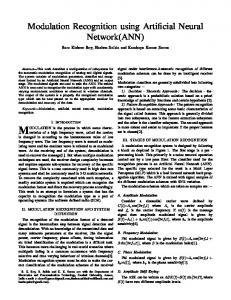
SVM CLASSIFIER Support vector machine (SVM) is a structural risk based learning machine, which constructs Ndimensional hyperplane to optimally separate the input data into different categories. A sigmoid kernel function model of SVM is equivalent to a two-layer, feed-forward neural network. Furthermore, SVM can use polynomial function or radial basis function (RBF) in which the weights of the network are found by solving a quadratic programming problem with linear constraints [8]. So we have proposed a multiclass SVM-based classifier (MCSVM) as Figure 1 that has a hierarchical structure. SVMs were introduced on the foundation of statistical learning theory. Since the middle of 1990s, the algorithms used for SVMs started emerging with greater availability of computing power, paving the way for numerous practical applications. The basic SVM deals with two-class problems; however, it can be developed for multiclass classification. The following subsections briefly describe the binary SVM and MCSVM.
Class 1 Vs Classes 2,3,4,5
1 Class 2 Vs Classes 3,4,5
ɸ(x)
2
Class 3 Vs Classes 4,5
3 Class 4 Vs Class 5
5
4
Figure 1. The proposed a multiclass SVM-based classifier (MCSVM) Support Vector Machine (SVM) is an empirical modeling algorithm and is the state-of-the-art for the existing classification methods. The SVM is basically a two-class classifier based on the ideas of “large margin” and “map- ping data into a higher dimensional space”, and the kernel functions in the SVM. The first objective of the SVM classification is the maximization of the margin between the two nearest data points belonging to two separate classes. The second objective is to constraint that all data points belong to the right class. It is a two-class solution which can use multi- dimension features. The two objectives of the Support Vector Classifier (SVC) problem are then incorporated into an optimization problem. SVC classifies the points from two linearly separable sets in two classes by solving a quadratic optimization problem in order to find the optimal separating hyper plane between these two classes. This hyper plane maximizes the IJECE Vol. 5, No. 3, June 2015 : 429 – 435
IJECE
ISSN: 2088-8708
433
distance from the convex hulls of each class. These techniques can be extended to the nonlinear cases by embedding the data in a nonlinear space using kernel functions. The robustness of SVC originates from the strong fundamentals of statistical learning theory. SVC can be applied to separable and non-separable data points. In the non-separable case, the algorithm adds one more design parameter. This parameter is the weight of the error caused by the points present in the wrong class region. In MC, this issue occurs in the low SNR cases. Another degree of freedom in the method we used in this paper to classify 5 modulation techniques, first we classify one class from the others and if the received signal features (which be- long to one class of 5 classes) does not belong to the single class and belongs to the other class, we remove the single class and take one class from the other classes and classify it from the rest of other classes and so on until we correctly classify the received signal [9].
5.
FEATURE ANALYSIS From Figure 2 that shows the first ten harmonics of all modulation schemes under studying where it seems not interference between them especially at the first harmonics. So these features will be leads to ease of the SVM to classify the signal that have these harmonics. Also with a deep analysis of modified covariance method where the increasing of the order p this lead to increase the recognition rate but the execution time becomes long at high value of p.
100 FSK2 FSK4 FSK8 FSK16 FSK64
95
Rate of 90 Recog nition 85
80
75 -15
-14
-13
-12
-11
-10
-9
-8
-7
-6
-5
Figure 2. The first ten harmonics of all modulation schemes Power spectral estimation by modifies covariance method used to generate the feature vectors, where data base of the signature modulation signal are generated. After this, the first ten harmonics of each feature observation and save it. Then used these features as input for SVM classifier in order to train SVM. The reason that leads to choose the first ten harmonics is that the interference between classes increase as we get towords the harmonics that have high order. So the choosing of harmonics will be restricts on the first ten only. Modulation identification includes inter-class classification for FSK with 5 class classification problem based on SVM. The structure of the hierarchical classifier is as shown in Figure 3. Firstly, we extract FSK2 from all, then FSK4 from the rest and so on.
Automatic Modulation Recognition for MFSK Using Modified Covariance Method (Hanan M. Hamee)
434
ISSN: 2088-8708
16
FSK2 FSK4 FSK8 FSK16
Magnitude of PSD
14
12
10
8
6
4
1
2
3
4
5
6
7
8
9
10
Figure 3. The structure of the hierarchical classifier
6.
RESULTS AND DISCUSSION The proposed algorithm was verified and validated for various orders of digitally modulated signals (BFSK, QFSK, 8FSK, 16FSK and 64FSK) in the presence of noise. Here the work gives a high rate of classification and good results that satisfies the goal of this work, where the recognition rate reaches to higher level and can be increased at more low of SNR by applying the optimization techniques for the parameters of SVM classifier .All the simulation steps for the digitally modulated signals, the feature extraction, training of the SVM and performance evaluation were developed using MATLAB. The proposed classifier has shown an excellent performance in noise presence and without any optimization for SVM parameters. In the training phase, 5 modulated signals of different orders are fed to the feature extraction feature Secondly, classification process that can be used to distinguish between 5 digital FSK modulations. Figure 4 gives imagination about the efficiency of this feature to recognize between different indexes of FSK. Where can that power spectral estimation by modified covariance method a strong tool in modulation recognition world.
100 FSK2 FSK4 FSK8 FSK16 FSK64
Rate of Recognition
95
90
85
80
75 -15
-14
-13
-12
-11
-10
-9
-8
-7
-6
-5
Signal to noise ratio (dB) Figure 4. Recognition rate at different SNRs for various modulation schemes when features extracted from the signal, p=30.
IJECE Vol. 5, No. 3, June 2015 : 429 – 435
IJECE
ISSN: 2088-8708
435
So from comparative between this work and others where in [10], the rate of recognition at 0dB for MFSK reaches to 94%. In [11] by using autoregressive approaches that gives a rate of recognition 95% after 0dB for FSK2, FSK4 only. Table 1 shows the rate of modulation recognition at -5 dB, Figure 4 shows the percentage of modulation recognition at different level of SNR (-15, -10, -5) dB Table 1. MFSK modulation recognition at SNR=-5dB Training set 1000 samples/class, Testing set 1000 samples/class, p=30. Type of modulation
FSK2
FSK2
1000
FSK4 FSK8 FSK16 FSK64
FSK4
FSK8
FSK16
FSK64
1000 1000 1000 1000
7.
CONCLUSION AND FUTURE WORK From the above results can be conclusion that this tools very well for MFSK modulation recognition at low SNR. The rate of recognition reaches to 97% at SNR=-10dB. So ther are many think that can be made in this topic as a future work one of them which it can be improved the rate of recognition by applying of optimization techniques for the parameters of the SVM . Also applied this method to another type of modulation such as PSK and QAM or any type of modulation and make a decision about its interests and other facts.
REFERENCES [1] Khandker Nadya Haq, Ali Mansour, Sven Nordholm, “Recognition of Digital Modulated Signals based on Statistical Parameters”, 4th IEEE International Conference on Digital Ecosystems and Technologies (IEEE DEST, 2010) . [2] Ataollah Ebrahimzadeh Shermeh, Reza Ghazalian, “Recognition of communication signal types using genetic algorithm and support vector machines based on the higher order statistics”, Elsevier, Digital Signal Processing, 20 (2010) 1748–1757. [3] Li Cheng1 and Jin Liu, “Automatic Modulation Classifier Using Artificial Neural Network Trained by PSO Algorithm”, Journal of Communications, 2013, 8(5). [4] Lei Huo, Tiandong Duan, Xiangqian Fang, “A Novel Method of Modulation Classification for Digital Signals”, International Joint Conference on Neural Networks Sheraton Vancouver Wall Centre Hotel, Vancouver, BC, Canada, 2006, 16-21. [5] Qu Jun-suo, “A Algorithm of Fast Digital Phase Modulation Signal Recognition”, TELKOMNIKA, 2012, 10(8), pp. 2330~2335 [6] P. Sasikiran, T. Gowri Manohar, S. Koteswara Rao, “Estimating the power spectrum of a wide sense Stationary random process using parametric approaches (AR, MA)”, International Journal of Recent Advances in Engineering & Technology (IJRAET). 2014, 2(2). [7] Lubna Badri and Mujahid Al-Azzo, “Modelling of long wavelength detection of objects using Elman network modified covariance combination”, The International Arab Journal of information technology, 2008, 5(3), pp. 265272. [8] Yu Wang, “Ultrasonic Flaw Signal Classification using Wavelet Transform and Support Vector Machine”, TELKOMNIKA, 2013, 11(12). [9] Mohamed El-Hady Magdy Keshk1, El-Sayed Elrabie, Fathi El-Sayed Abd El-Samie, Mohammed Abd El-Naby, “Blind Modulation Recognition in Wireless MC-CDMA Systems Using a Support Vector Machine Classifier”, Wireless Engineering and Technology,2013,4,145-153, Published on (http://www.scirp.org/journal/wet). [10] Sajjad Ahmed Ghauri, Ijaz Mansoor Qureshi, Ihtesham Shah and Nasir Khan, “Modulation Classification using Cyclostationary Features on Fading Channels”, Research Journal of Applied Sciences, Engineering and Technology 2014, 7(24), pp. 5331-5339. [11] He Ji-ai, Liu Huan, Li Ying-tang, Ding Li-qi, Wang Jie, “Modulation Recognition Based on Feature Extraction by AutoRegressive Model”, TELKOMNIKA Indonesian Journal of Electrical Engineering 2014, 12(3), pp. 1911 ~ 1916.
Automatic Modulation Recognition for MFSK Using Modified Covariance Method (Hanan M. Hamee)