IEEE TRANSACTIONS ON SPEECH AND AUDIO PROCESSING, VOL. 13, NO. 3, MAY 2005
441
Automatic Music Classification and Summarization Changsheng Xu, Senior Member, IEEE, Namunu C. Maddage, and Xi Shao
Abstract—Automatic music classification and summarization are very useful to music indexing, content-based music retrieval and on-line music distribution, but it is a challenge to extract the most common and salient themes from unstructured raw music data. In this paper, we propose effective algorithms to automatically classify and summarize music content. Support vector machines are applied to classify music into pure music and vocal music by learning from training data. For pure music and vocal music, a number of features are extracted to characterize the music content, respectively. Based on calculated features, a clustering algorithm is applied to structure the music content. Finally, a music summary is created based on the clustering results and domain knowledge related to pure and vocal music. Support vector machine learning shows a better performance in music classification than traditional Euclidean distance methods and hidden Markov model methods. Listening tests are conducted to evaluate the quality of summarization. The experiments on different genres of pure and vocal music illustrate the results of summarization are significant and effective. Index Terms—Clustering, music characterization, music classification, music summarization, support vector machines.
I. INTRODUCTION
T
HE RAPID development of various affordable technologies for multimedia content capturing, data storage, high bandwidth/speed transmission, and the multimedia compression standards such as JPEG and MPEG, have resulted in a rapid increase of the size of digital multimedia data collections and greatly increased the availability of multimedia contents to the general user. Digital music is one of the most important data types distributed by the Internet. However, it is still difficult for a computer to automatically analyze music content, especially to automatically classify and recognize music content. Since lyrics provide important information in the music, it would be very useful if we could automatically discriminate pure music and vocal music and then detect vocal parts from vocal music. It can be applied to music classification and content-based music retrieval. We cannot use speech recognition techniques to detect singing voice from vocal music because singing voice is much more complicated than pure speech. How to detect and extract the singing voice from vocal music is a challenge in music content analysis. A number of methods have been proposed to discriminate music, speech, silence, and environment sound. The most successful achievement in this area is speech/music discrimination,
Manuscript received June 9, 2003; revised January 7, 2004. The associate editor coordinating the review of this manuscript and approving it for publication was Dr. Michael Davies. The authors are with the Institute for Infocomm Research, Singapore 119613 (e-mail:
[email protected];
[email protected];
[email protected]). Digital Object Identifier 10.1109/TSA.2004.840939
because speech and music are quite different in spectral distribution and temporal change pattern. Saunders [1] used the average zero-crossing rate and the short time energy as features and applied a simple thresholding method to discriminate speech and music from the radio broadcast. Scheirer and Slaney [2] used thirteen features in time, frequency and cepstrum domains and different classification methods to achieve a robust performance. Both approaches reported accuracy rate for real-time classification over 95% if a window size of 2.4 s was used. However, the performance will decrease for the above approaches if a small window size is used or other audio scenes such as environment sounds are taken into consideration. Further research works have been done to segment audio data into more categories. El-Maleh et al. [3] proposed a method to classify audio signals into speech, music, and others for the purpose of parsing of news story. Kimber and Wilcox [4] proposed an acoustic segmentation approach that mainly applied to the segmentation of discussion recordings in meetings. Audio recordings were segmented into speech, silence, laughter and nonspeech sounds by using cepstral coefficients as features and a hidden Markov model (HMM) as the classifier. The accuracy rate depended on different types of recording. Zhang and Kuo [5] proposed an approach to divide the generic audio data segmentation and classification task into two stages. In the first stage, audio signals were segmented and classified into speech, music, song, speech with music background, environmental sound with music background, six types of environmental sound, and silence. In the second stage, further classification was conducted within each basic type. Speech was differentiated into the voice of man, woman and child. Music is classified into classics, blues, jazz, rock and roll, music with singing and the plain song, according to the instruments or types. Environmental sounds were classified into semantic classes such as applause, bell ring, footstep, wind-storm, laughter, bird’s cry, and so on. The accuracy rate was reported over 90%. Lu et al. [6] proposed a robust two-stage audio classification and segmentation method to segment an audio stream into speech, music, environment sound and silence. The first stage of classification was to separate speech from nonspeech based on K-nearest-neighbor (KNN) and linear spectral pairs—vector quantization (LSP-VQ) classification scheme and simple features such as zero-crossing rate ratio, short time energy ratio, spectrum flux, and LSP distance. The second stage further segmented the nonspeech class into music, environment sounds and silence with a rule-based classification scheme and two new features: noise frame ratio and band periodicity. The total accuracy rate was reported over 96%. How to create a concise and informative extraction that best summarizes an original digital content is another challenge in music content analysis and is extremely important in large-scale information organization and processing. Nowadays, most of
1063-6676/$20.00 © 2005 IEEE Authorized licensed use limited to: FLORIDA INTERNATIONAL UNIVERSITY. Downloaded on July 29,2010 at 19:49:40 UTC from IEEE Xplore. Restrictions apply.
442
IEEE TRANSACTIONS ON SPEECH AND AUDIO PROCESSING, VOL. 13, NO. 3, MAY 2005
Fig. 1. Block diagram for calculating LPC and LPCC coefficients.
the summarization for commercial use is manually produced from the original content. However, since a large volume of digital content has been made publicly available on mediums such as the Internet during recent years, efficient ways of automatic summarization have become increasingly important and necessary. So far, a number of techniques have been proposed to automatically generate text [7], [8], speech [9], [10] and video [11]–[13] summaries. Similar to text, speech, and video summarization, music summarization refers to determining the most common and salient themes of a given music that may be used as a representative of the music and readily recognized by a listener. Automatic music summarization can be applied to music indexing, content-based music retrieval and web-based music distribution. Several research methods are proposed in automatic music summarization. A music summarization system [14] was developed on MIDI format, which utilized the repetition nature of MIDI compositions to automatically recognize the main melody theme segment of a given piece of music and generate music summary. But MIDI is a synthesizer and structured format and is different from sampled audio format such as wav which is highly unstructured. Therefore, MIDI summarization method cannot be applied to real music summarization. A real music summarization system [15] used mel frequency cepstral coefficients (MFCCs) to parameterize each music song. Based on MFCCs, a cross-entropy measure, or HMM, was used to discover the song structure. Then heuristics were applied to extract the key phrase in terms of this structure. This summarization method is suitable for certain genres of music such as rock or folk music, but it is less applicable to classical music. MFCCs were also used as features in Cooper and Foote’s works [16]. They used a two-dimensional (2-D) similarity matrix to represent music structure and generate music summary. But this approach will not always yield intuitively piece. Peeters et al. [17] proposed a multi-pass approach to generate music summaries. The first pass used segmentation to create “states”. The second pass used these states to structure music content by unsupervised learning (HMM). The summary was constructed by choosing a representative example of each state. The generated summary can be further refined by an overlap-add method and a tempo detection/beat alignment algorithm. But there were no evaluations for the quality of the generated summaries. In this paper, novel automatic music classification and summarization approaches are presented. In order to discriminate pure and vocal music, a support vector machine (SVM) is applied to obtain the optimal class boundary between pure and vocal music by learning from training data. For pure and vocal music, a number of features are extracted to characterize music
content, respectively. These features are used to structure the music content by use of a clustering algorithm. Summaries of pure and vocal music are created based on the clustering result and domain-related music knowledge. Experimental results show this method can provide a better summarization result than current existing methods. The rest of this paper is organized as follows. The pure and vocal music classification approach is presented in Section II, including music characterization, SVM learning and a classification scheme. Pure and vocal music summarization schemes are described in detail in Section III. Experimental results of SVM learning and user evaluation are reported in Section IV. Finally, conclusions and future work are given in Section V. II. MUSIC CLASSIFICATION It is important to classify the music into pure music and vocal music before summarizing it, because different features will be used for pure and vocal music, respectively. Pure music is defined as the music containing only instrumental music, while vocal music is defined as the music containing both vocal and instrumental music. A. Music Characterization Feature selection is important for music content analysis. The selected features should reflect the significant characteristics of different kinds of music signals. In order to better classify pure and vocal music, we consider the features that are related to vocal signals. The selected features include linear prediction coefficients (LPC)-derived cepstrum coefficients (LPCC) and zero-crossing rates (ZCR). 1) LPC and LPCC: LPC and LPCC are two linear prediction methods [18] and they are highly correlated to each other. Our experiment shows that LPCC is much better than LPC in identifying vocal music. The performance of LPC and LPCC can be improved by 20%–25% by filtering the full-band music signal (0–22 025 Hz with 44.1-kHz sampling rate) into sub frequency bands and then down-sampling the subbands before calculating the coefficients. The subbands are defined according to lower, middle, and higher musical scales [19], as shown in Fig. 1. Frequency ranges for the designed filter banks – , – , – , are – , – , – , – , – , – , and – . Therefore, calculating LPC coefficients for different frequency bands can represent dynamic behavior of spectrums of selective frequency bands (i.e., different octave of music).
Authorized licensed use limited to: FLORIDA INTERNATIONAL UNIVERSITY. Downloaded on July 29,2010 at 19:49:40 UTC from IEEE Xplore. Restrictions apply.
XU et al.: AUTOMATIC MUSIC CLASSIFICATION AND SUMMARIZATION
Fig. 2.
443
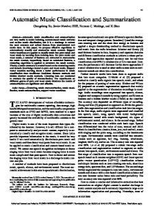
Third LPC and LPCC coefficient of 220.5–441-Hz filter bank. (a) Vocal music. (b) Pure music.
Fig. 3. Zero-crossing rates (0–276 frames for vocal and 276–592 frames for pure music).
Fig. 2 shows the third order of LPC and LPCC generated in a 220.5–441-Hz filter bank. The variance of LPCC is much lower than LPC in both vocal music (female vocals) and pure music (guitar). This implies that spread of LPCC is closer to mean of LPCC than the spread in LPC. For the same class of music, the robust feature should not vary much around the mean value and ideally the variation is zero. Thus, LPCC is more robust than LPCC. 2) Zero-Crossing Rates: Zero-crossing rates are usually suitable for narrowband signals [19], but music signals include both narrowband and broadband components. Therefore, the short time zero crossing rates can be used to characterize music signal. The N-length short-time zero-crossing rates are defined as
(1)
is a rectangular window. where Fig. 3 is an example of zero-crossing rates for pure and vocal music. It can be seen that vocal music has high zero-crossing rates. This feature is sensitive to vocals (i.e., strong harmonic structure) and percussion instruments with lower decaying time.
B. Music Classification 1) SVMs: SVM learning is a useful statistic machine learning technique that has been successfully applied in the pattern recognition area [20], [21]. If the data are linearly nonseparable but nonlinearly separable, the nonlinear support vector classifier will be applied. The basic idea is to transform input vectors into a high-dimensional feature space using a nonlinear transformation , and then to do a linear separation in feature space (see Fig. 4). To construct a nonlinear support vector classifier, the inner is replaced by a kernel function product (2) The learning scheme is shown in Fig. 5. The SVM has two layers. During the learning process, the first layer selects the , (as well as the number ), from the basis given set of bases defined by the kernel; the second layer constructs a linear function in this space. This is completely equivalent to constructing the optimal hyperplane in the corresponding feature space. The SVM algorithm can construct a variety of learning machines by use of different kernel functions. Three kinds of kernel functions are usually used. They are as follows.
Authorized licensed use limited to: FLORIDA INTERNATIONAL UNIVERSITY. Downloaded on July 29,2010 at 19:49:40 UTC from IEEE Xplore. Restrictions apply.
444
IEEE TRANSACTIONS ON SPEECH AND AUDIO PROCESSING, VOL. 13, NO. 3, MAY 2005
Fig. 4.
Nonlinear SVM.
Fig. 6. SVM learning process.
Fig. 5.
Scheme of SVMs. Fig. 7. Music identification.
1) Polynomial kernel of degree (3) 2) Radial basis function with Gaussian kernel of width
(4) 3) Neural networks with tanh activation function (5) where the parameters and are the gain and shift. Our earlier experiments show that Radial basis function performed better for musical signal classification [22]. 2) SVM Learning and Music Classification: We use a nonlinear support vector classifier to discriminate pure and vocal music. Classification parameters are calculated using support vector machine learning. Fig. 6 illustrates a conceptual block diagram of the training process to produce classification parameters. The training process analyzes music training data to find an optimal way to classify musical frames into pure or vocal class. The training data should be sufficient to be statistically significant. The training data is segmented into fixed-length and overlapping frames (in our experiments we used 20 ms frames with 50% overlapping). When neighboring frames are overlapped, the temporal characteristics of music content can be taken into consideration in the training process. Features such as LPCC and ZCR are calculated from each frame. The support vector machine learning algorithm is applied to produce the classification parameters according to calculated features. The training process needs to be performed only once. The derived classification parameters are used to classify pure and vocal music.
Fig. 8.
Block diagram of music summarization.
The music content can be discriminated into pure and vocal music in terms of the designed support vector classifier (see Fig. 7). III. MUSIC SUMMARIZATION Fig. 8 conceptually illustrates the main components of music summarization. The music content is first preprocessed by removing silence and being segmented into fixed-length and overlapping frames. Then the feature extraction is conducted in each frame. Based on the calculated features, a clustering algorithm is applied to group these frames to get the structure of the music content. Finally, a music summary is created based on clustered results and music domain knowledge. Each of these components will be described in Sections III-A–D. The summarization process for pure and vocal music is similar, but there are several differences. The first difference is feature extraction. We use different feature set to characterize pure
Authorized licensed use limited to: FLORIDA INTERNATIONAL UNIVERSITY. Downloaded on July 29,2010 at 19:49:40 UTC from IEEE Xplore. Restrictions apply.
XU et al.: AUTOMATIC MUSIC CLASSIFICATION AND SUMMARIZATION
445
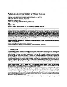
Fig. 9. Behaviors of the first, 15th, and 20th MFCCs of pure and vocal music. (a) Vocal music. (b) Pure music.
and vocal music content, respectively. The second difference is summary generation. For pure music, the summary is still pure music. However, for vocal music, the summary should start with vocal part and it is desirable to have the music title sung in the summary. For vocal music, there are some other rules relevant to music genres. In pop and rock music, the main melody part typically repeats in the same way without major variations. The pop and rock music usually follows a similar scheme, for example, ABAB format where A represents a verse and B represents a refrain. The main theme (refrain) part occurs the most, followed by the verse, bridge and so on. However, jazz music usually comprises the improvization of the musicians, producing variations in most of the parts and creating problems in determining the main melody part. There is no refrain in jazz music and the main part is the verse. A. Preprocessing The aim of preprocessing is to remove silence from a music sequence. Silence is defined as a segment of imperceptible music, including unnoticeable noise and very short clicks. We use short-time energy to detect silence. The short-time energy function of a music signal is defined as
1) Mel Frequency Cepstral Coefficients: The mel-frequency cepstrum has proven to be highly effective in recognizing structure of music signals and in modeling the subjective pitch and frequency content of audio signals. Psychophysical studies have found the phenomena of the mel pitch scale and the critical band, and the frequency scale-warping to the mel scale has led to the cepstrum domain representation. The mel scale is defined as (8) where is the logarithmic scale of normal frequency scale. The mel-cepstral features can be illustrated by the MFCCs, which are computed from the fast Fourier transform (FFT) power coefficients. The power coefficients are filtered by a triangular bandpass filter bank. When in (8) is in the range of 250–350, the number of triangular filters that fall in the frequency range (200–1200) Hz (i.e., the frequency range of dominant music information) is higher than the other values of . Therefore, it is efficient to set the value of in that range for calculating MFCCs. Denoting the output of the filter bank by , the MFCCs are calculated as
(6) where is the discrete time music signal, is the time index is a rectangular window, i.e., of the short-time energy, and otherwise.
(7)
If the short-time energy function is continuously lower than a certain set of thresholds (there may be durations in which the energy is higher than the threshold, but the durations should be short enough and far apart from each other), the segment is indexed as silence. Silence segments will be removed from the music sequence. The processed music sequence will be segmented into fixed length and 50% overlapping frames. B. Feature Selection For pure music, power-related features such as mel-frequency ceptrum coefficients, amplitude envelope, and power spectrum are used. For vocal music, voice-related features such as LPC derived cepstrum coefficients, zero-crossing rate, spectrum flux, and cepstrum flux are used.
(9) Fig. 9(a) and (b) illustrate the behaviors of the first, 15th, and 20th MFCCs of vocal and pure music, respectively. Initially both music samples were segmented into nonoverlapping 20 ms frames and then 20 MFCCs were calculated with 20 triangular filters. In Fig. 9(a), 0 to 1150 frames (X) belong to piano mixed vocal music, 1151 to 3870 frames (Y) are piano, drums, and guitar-mixed vocal music, and the rest (Z) is guitar-mixed vocal music. The first 1048 frames in Fig. 9(b) belong to piano music and the rest belongs to mixed instrumental music (Drums, Piano and Guitar music). It can be seen that MFCCs respond better for pure music [Fig. 9(b)] than vocal music [Fig. 9(a)]. 2) Spectrum Flux: Spectrum flux is defined as the variation value of spectrum between the adjacent two frames (10) where is the magnitude of the FFT of the th frame at frequency bin . Both magnitude vectors are normalized in energy. Spectrum flux is a measure of spectral change.
Authorized licensed use limited to: FLORIDA INTERNATIONAL UNIVERSITY. Downloaded on July 29,2010 at 19:49:40 UTC from IEEE Xplore. Restrictions apply.
446
IEEE TRANSACTIONS ON SPEECH AND AUDIO PROCESSING, VOL. 13, NO. 3, MAY 2005
3) Cepstrum Flux: Similar to spectrum flux, cepstrum flux is defined as the norm of difference between the cepstrum of the successive frame (11) 4) Spectral Power: For a music signal weighted with a Hanning window
denotes amplitude envelop, denotes the denotes the linear prediction cepstrum coefficients, denotes the spectrum flux, and zero-crossing rates, denotes the cepstrum flux. 3) Calculate the distances between every pair of music frames and using the Mahalanobis distance [24]
, each frame is (14) where Since
is the covariance matrix of the feature vector. is symmetric, it can be diagonalized as , where is a diagonal matrix and is an orthogonal matrix. So (14) can be simplified in terms of Euclidean distance as follows:
(12) where is the number of samples of each frame. The spectral is calculated as power of the signal
(15)
(13) The maximum is normalized to a reference sound pressure level of 96 dB. 5) Amplitude Envelop: The amplitude envelope describes the energy change of the signal in the time domain and is generally equivalent to the so-called ADSR (attack, decay, sustain, release) of a musical sound. The envelope of the signal is computed with a frame by frame root mean square (rms) and a low third-order Butterworth lowpass filter [23]. The length of the rms frame determines the time resolution of the envelope. A large frame length yields lower transient information and small frame length greater transient energy. The cutoff frequencies of the Butterworth low pass filter , 1200 Hz are determined empirically at 350 Hz , and 1700 Hz . C. Clustering The aim of the music summarization is to analyze a given music sequence and extract the important frames to reflect the salient theme of the music. Based on calculated features of each frame, we use an adaptive clustering method to group the music frames and obtain the structure of the music content. Since the adjacent frames have overlap, the length of overlap is very important for frame grouping. In the initial stage, it is difficult to determine the length of overlap exactly. But we can adaptively adjust the length of overlap if the clustering result is not ideal for frame grouping. The clustering algorithm is described as follows. 1) Segment the music signal (pure or vocal music) into fixed-length ( is 20 ms, in this case) and overlapping frames and label each frame with a number , where the overlapping rate , 1, 2, 3, 4, 5, 6). ( 2) For each frame, calculate music features to form a feature vector. For pure music, the th feature vector is constructed and for as vocal music it is , where denotes the mel-frequency denotes the spectral power, cepstral coefficient,
The complexity of the computation of the vector distance to . can be reduced from 4) Embed the calculated distances into a 2-D representation shown in Fig. 10. The matrix contains the similarity metric calculated for all frame combinations, hence th element of frame indexes and such that the is . 5) Normalize matrix according to the highest distance between frames. i.e., . 6) For a given , calculate the summation of total distance between all the frames, denoted as , which is the defined as the following: (16) 7) Repeat steps 1)–6) by varying from 1 to 6 and find an optimal which can give the maximum value for 8) Do agglomerative hierarchical clustering [25] Here, we consider putting music frames into clusters
.. . .. . .. .
Procedure ^ = n, V ~ ^ is the 1 Let C Hi , i = 1; . . . ; n where C i initial number of clusters and Hi denotes the ith cluster. Initially, each cluster contains one frame.
2
Authorized licensed use limited to: FLORIDA INTERNATIONAL UNIVERSITY. Downloaded on July 29,2010 at 19:49:40 UTC from IEEE Xplore. Restrictions apply.
XU et al.: AUTOMATIC MUSIC CLASSIFICATION AND SUMMARIZATION
447
D. Summary Generation After the clustering, the structure of the music content can be obtained. Each cluster contains frames with similar features. A summary can be generated based on this structure and domainspecific musical knowledge. According to music theory, the most distinctive or representative musical themes should repetitively occur in an entire music work [26]. Based on this musical knowledge and clustering results, the summary of a music work can be generated as follows. ; the number Let us assume summary length of clusters is ; the length of a music frame is ms. 1) Total number of music frames in the summary (19)
Fig. 10.
Distance matrix of frames.
^ = C , stop. C is the desired number of 2 If C
clusters. The optimal desired number of clusters is defined as following: C3 = k 1
Lsum Tc3
(17)
(20)
where Lsum is the time length of music summary (in seconds) and Tc3 is the minimum time length of subsummary (in seconds) made in a cluster (see Section III-D for detail). Thus, dLsum =Tc3 e is the actual number of subsummary required to construct the summary. k is a magnification constant selected in the experiment and it is better to select k times more clusters than the required number of clusters, because it can guarantee enough clusters to be selected in summary. Our experiments have shown that the ideal time length of a subsummary is between 3 and 5 s. A playback time shorter than 3 s results in a nonsmooth and even nonacceptable music, while a playback time longer than 5 s results in a lengthy, rhythm reparative, and slow-paced one. Thus, Tc3 = 3 has been selected for our experiments. 3 Find “nearest” pair of distinct clusters,
Hi and Hj where i and j are cluster indexes ^ 4 Merge Hi and Hj , delete Hj , and C
C^ 0 1. 5 Go to step 2 .
At any level, the distance between nearest clusters can be used as similarity values for that level. Distance similarity measures can be calculated by (18) where
and
are mean value of the cluster
2) According to the cluster mean distance matrix, we can arrange clusters in descending order and clusters with higher distance are selected for making the summary. 3) Subsummaries are made within the cluster. Selected frames in the cluster must be as continuous as possible and the length of the combined frames within the cluster should be 3–5 s or the number of frames should be frames and frames, where between
and
.
and (21) Assume and are the first frame and last frame in and time domain of a selected cluster such that . From music knowledge and our experiments, a piece of discontinuous music (less than 3 s) is not acceptable for human ears. Hence, we should make the subsummaries continuous. If frames are discontinuous between frame and frame , we add the frames between and , make the frames in this cluster continuous, and at the same time delete these added frames from other clusters. Then, we to adjust the summary follow the condition , , or length within the cluster. , as Fig. 11(a) shows, we add Condition : frames to the head and tail until the subsummary length is equal to . Assume represents the number of the added frames before (i.e., tail frames), and represents the number of the added frames after (i.e., head frames). If the added frames exceed the end frame or starting frame of the original music, exceeding frames will be added to tail frames (22) or head frames (23), respectively (22) (23)
Authorized licensed use limited to: FLORIDA INTERNATIONAL UNIVERSITY. Downloaded on July 29,2010 at 19:49:40 UTC from IEEE Xplore. Restrictions apply.
448
IEEE TRANSACTIONS ON SPEECH AND AUDIO PROCESSING, VOL. 13, NO. 3, MAY 2005
Fig. 11.
Subsummaries generation.
where is the total number of frames in music, and , represents the number of the added frames before and after after adjusting. Condition : As Fig. 11(b) shows, no change in the subsummary length and it is equal to . : , as Fig. 11(c) shows, we Condition delete frames both from the head frame and tail frame until the subsummary length is equal to . 4) Repeat step 3) to make individual subsummaries for selected clusters and stop the process when summation of subsummary lengths equals or is slightly greater than the required summary length. 5) If the summary length exceeds the required length then find the subsummary length, which is more than 3 s and adjust its length to get the final summary length. 6) Merge those subsummaries according to their positions in the original music to get the final summary. IV. EXPERIMENTS To illustrate and evaluate our proposed music classification and summarization algorithms, experiments are conducted for various genres of pure and vocal music samples. For music classification, we use SVM learning to classify pure and vocal music and give a comparison between the SVM method, traditional Euclidean distance method and HMM method. For music summarization, we test our algorithm on different genres of music samples and perform a user listening evaluation. The experimental results are promising. A. Pure and Vocal Music Classification The music dataset used in music classification experiment contains 100 music samples including 50 pure music samples and 50 vocal music samples. They are collected from music CDs and the Internet and cover different genres such as pop, classical, rock and jazz. All data are 44.1-kHz sample rate, stereo channels and 16 bits per sample. In order to make training results statistically significant, training data should be sufficient and cover various genres of music. We select 35 music samples as a training set, including five pop pure music, five pop vocal music, five classical pure music, five classical vocal music, five rock
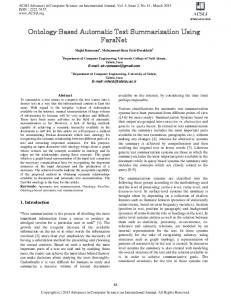
Fig. 12.
Number of frames versus number of support vectors.
pure music, five rock vocal music, and five jazz vocal music. Each sample is segmented into 2000 frames and the length of each frame is 882 sample points. Therefore, the total number of training data is 70 000 frames including 31 349 vocal frames and 38 651 pure music frames (some frames are pure music in a vocal music sample). The rest of the samples are used as a test set. [in (2)] is used as the A radial basis function with kernel in SVM training and classification. The training data of and vocal and pure music frames are assigned to classes , respectively. From Fig. 12, we can see that the gradient of the curve decreases with number of test data frames. When proper pure and vocal music frames are used as training data, the gradient may tend to zero and the number of support vectors may tend to a constant value. After training the SVM, we use it as the classifier to classify vocal and pure music frames on the test set. The test set is divided into three parts. The first part contains 20 pure music samples (40 000 frames). The second part contains 20 vocal music samples (40 000 frames). The third part contains 15 pure music samples and ten vocal music samples (50 000 frames). The test data are tested using SVM. For comparison, we also test the data using a traditional nearest neighbor (NN) method and an HMM method. The traditional NN classifier we used here is similar to the - nearest neighbor classifier described in [27]. For the HMM classifier, we adopt the same approach described in [28], which has fivestates including entry and exit states, and for each state, a 4-component mixture Gaussian distribution is used. Table I shows a comparison between the three methods. It can be seen that SVM achieves a significantly higher accuracy rate than NN and HMM.
Authorized licensed use limited to: FLORIDA INTERNATIONAL UNIVERSITY. Downloaded on July 29,2010 at 19:49:40 UTC from IEEE Xplore. Restrictions apply.
XU et al.: AUTOMATIC MUSIC CLASSIFICATION AND SUMMARIZATION
TABLE I SVM AND NN FOR MUSIC SEPARATION
449
TABLE II MARKS DISTRIBUTION OF MUSIC SUMMARY
B. Summarization Evaluation Since there is no ground truth available to evaluate the quality of a music summary, we employed a subjective user study [29] to evaluate the performance of our music summarization method. Four genres of pure and vocal music are used in the test. They are pop, classical, rock and jazz. Each genre contains five musical samples with stereo, 16 bits/sample and 44.1-kHz sample rates. The length of musical testing samples varies from 3 to 5 min. The length of the summary for each sample is 30s. Ten subjects were invited for evaluation. Before the tests, the subjects could listen to each original music for many times in order to become familiar with the theme of the music. Some of the characteristics of music summary are listed below. a) Clarity: This pertains to the clearness and comprehensibility of the music summary. b) Conciseness: This pertains to the terseness of the music summary and how much of the summary captures the essence of the original music work. c) Coherence: This pertains to the consistency and natural drift of the segments in the music summary. The subjects were asked to listen to summaries generated from testing samples and rated the summaries in the above three categories on a grade of 1–5, corresponding to worst and best, respectively. The expected summary should include characteristics of the original music and the summary could highlight the same emotions of the original music. The average grade of summaries in each genre from all subjects is the final grade of this genre. In order to make comparison, we also asked the subjects to rate the summaries using a nonadaptive clustering method [15] in terms of the same rules. In addition, to highlight the importance and necessity of music classification to the performance of music summarization, we also asked the subjects to rate the summaries using our proposed method without music classification. In this experiment, for the input music, we combine the two feature sets (one for pure and the other for vocal in the summarization with music classification) together to generate the music summary. Table II is an example mark sheet filled by one subject. The original music is a pop song named “Quit playing games with my heart” sung by the Backstreet Boys. All the characteristics of the original song are listed in the first column. In the second and third columns, the subject has noted his marks (1–5) after comparing characteristics present in the summaries generated according to both our method and nonadaptive clustering method, and the fourth column contains characteristics present in the summaries generated by our method without music classification. We employ the overall quality of the music as an attribute to evaluate a music summary because it pertains to the general perception or reaction of the users to the music summaries. The
TABLE III OVERALL RESULTS OF LISTENING EVALUATION
average grade of summaries in each genre from all subjects is the final grade of this genre. Overall evaluation results are listed in Table III. For every music sample there is a mark sheet like Table II, with average marks produced by every subject. Then we add all the average marks according to each genre and divide by the total number of music samples in one genre (5) and subjects (10). From the test results, it can be seen that the summaries using our method performed quite well with the score over 4 in all categories. It can also be seen that our method is superior to the nonadaptive clustering method for all genres of music testing samples. In addition, the results in Table III show that the classification stage in our proposed method is essential because it improved the performance of the final music summarization. Looking at the summarization performance of each genre, pop and rock music score highly, while scores of classical and jazz are relatively low. Usually, each repetition of the main melody comes with a small variation, also depending on the genre. In most of today’s pop and rock music, the main melody part repeats typically in the same way without major variations. However, classical and jazz music usually comprise the improvization of the musicians, producing variations in most of the parts and creating problems in determining the main melody part. V. CONCLUSION We have presented an automatic classification algorithm for pure and vocal music using support vector machine learning and an automatic summarization algorithm for pure and vocal music using adaptive clustering. Linear prediction cepstrum coefficients, zero-crossing rates, mel-frequency cepstral coefficients, spectral power, amplitude envelope, spectrum flux, and cepstrum flux are calculated as features to characterize music content. A nonlinear support vector machine learning algorithm is applied to obtain the optimal class boundary between pure and vocal music by learning from training data. An adaptive clustering method is applied to group music frames to structure
Authorized licensed use limited to: FLORIDA INTERNATIONAL UNIVERSITY. Downloaded on July 29,2010 at 19:49:40 UTC from IEEE Xplore. Restrictions apply.
450
IEEE TRANSACTIONS ON SPEECH AND AUDIO PROCESSING, VOL. 13, NO. 3, MAY 2005
music content according to calculated features. Music summary is generated based on the clustering result and domain-related music knowledge. The experimental results show that the support vector machine learning method has better performance in music classification than traditional Euclidean distance methods and HMM methods. The result of listening evaluation for our proposed music summarization algorithm is also encouraging and points to superiority over current existing methods. There are several directions that need to be explored in the future. The first direction is to improve the computational efficiency for support vector machines. Support vector machines take a long time in the training process, especially with a large number of training samples. Therefore, how to select proper kernel function and determine the relevant parameters is extremely important. The second direction we wish to investigate is to improve the accuracy of the summarization result. To achieve this goal, on the one hand, we need to explore more music features that can be used to characterize the music content; on the other hand, more domain-related music knowledge should be taken into consideration when generating music summary, especially for the genres of classical and jazz music. REFERENCES [1] J. Sounders, “Real-time discrimination of broadcast speech/music,” in Proc. ICASSP96, vol. 2, Atlanta, GA, 1996, pp. 993–996. [2] E. Scheirer and M. Slaney, “Construction and evaluation of a robust multifeature music/speech discriminator,” in Proc. ICASSP97, vol. 2, 1997, pp. 1331–1334. [3] K. El-Maleh, M. Klein, G. Petrucci, and P. Kabal, “Speech/music discrimination for multimedia application,” in Proc. ICASSP00, Istanbul, Turkey, Jun. 2000. [4] D. Kimber and L. Wilcox, “Acoustic segmentation for audio browsers,” in Proc. Interface Conf., Sydney, Australia, 1996. [5] T. Zhang and C.-C. Kuo, “Video content parsing based on combined audio and visual information,” in Proc. SPIE 1999, vol. 4, San Jose, CA, 1999, pp. 78–89. [6] L. Lu, H. Jiang, and H. J. Zhang, “A robust audio classification and segmentation method,” in Proc. ACM Multimedia 2001, Ottawa, ON, Canada, 2001. [7] Advances in Automatic Text Summarization, I. Mani and M. T. Maybury, Eds., MIT Press, Cambridge, MA, 1999. [8] F. Ren and Y. Sadanaga, An Automatic Extraction of Important Sentences Using Statistical Information and Structure Feature, 1998, vol. NL98–125, pp. 71–78. [9] K. Koumpis and S. Renals, “Transcription and summarization of voicemail speech,” in Proc. Int. Conf. Spoken Language Processing, Sydney, Australia, 1998. [10] C. Hori and S. Furui, “Improvements in automatic speech summarization and evaluation methods,” in Proc. Int. Conf. Spoken Language Processing, Sydney, Australia, 1998. [11] Y. Gong and X. Liu, “Summarizing video by minimizing visual content redundancies,” in Proc. IEEE Int. Conf. Multimedia and Expo, Tokyo, Japan, 2001, pp. 788–791. [12] I. Yahiaoui, B. Merialdo, and B. Huet, “Generating summaries of multiepisode video,” in Proc. IEEE Int. Conf. Multimedia and Expo, Tokyo, Japan, 2001, pp. 792–795. [13] C. M. Chew and M. Kankanhalli, “Compressed domain summarization of digital video,” in Advances in Multimedia Information Processing—PCM 2001, vol. 2195, Lecture Notes in Computer Science, Beijing, China, 2001, pp. 490–497. [14] R. Kraft, Q. Lu, and S. Teng, “Method and Apparatus for Music Summarization and Creation of Audio Summaries,” U.S. Patent 6 225 546, 2001. [15] B. Logan and S. Chu, “Music summarization using key phrases,” in Proc. IEEE Int. Conf. Audio, Speech and Signal Processing, Orlando, FL, 2000. [16] M. Cooper and J. Foote, “Automatic music summarization via similarity analysis,” in Proc. Int. Conf. Music Information Retrieval, Paris, France, 2002.
[17] G. Peeters, A. Burthe, and X. Rodet, “Toward automatic music audio summary generation from signal analysis,” in Proc. Int. Conf. Music Information Retrieval, Paris, France, 2002. [18] L. R. Rabiner and B. H. Juang, Fundamentals of Speech Recognition. Englewood Cliffs, NJ: Prentice-Hall, 1993. [19] J. R. Deller, J. H. L. Hansen, and J. G. Proakis, Discrete-Time Processing of Speech Signals. New York: Wiley, 1999. [20] T. Joachims, “Text categorization with support vector machines,” in Proc. European Conf. Machine Learning, Chemnitz, Germany, Apr. 1998. [21] C. Papageorgiou, M. Oren, and T. Poggio, “A general framework for object detection,” in Proc. Int. Conf. Computer Vision, Bombay, India, Jan. 1998. [22] C. Xu, N. C. Maddage, and Q. Tian, “Support vector machine learning for music discrimination,” in Proc. 3rd IEEE PCM 2002, Taiwan, Japan, pp. 928–935. [23] G. M. Ellis, Electronic Filter Analysis and Synthesis. Boston, MA: Artech House, 1994. [24] X. Sun, A. Divakaran, and B. S. Manjunath, “A motion activity descriptor and its extraction in compressed domain,” in Advances in Multimedia Information Processing—PCM 2001, Lecture Notes in Computer Science 2195, Beijing, China, 2001, pp. 450–457. [25] R. O. Duda, P. E. Hart, and D. G. Stork, Pattern Classification, 2nd ed. New York: A Wiley-Interscience Publication, 2000. [26] E. Narmour, The Analysis and Cognition of Basic Melodic Structures. Chicago, IL: University of Chicago Press, 1990. [27] K. D. Martin and Y. E. Kim, “Music instrument identification: A patternrecognition approach,” in 136th Meeting of ASA, Oct. 1998. [28] S. Gao, N. C. Maddage, and C. H. Lee, “A hidden Markov model based approach to music segmentation and identification,” in Proc. 4th IEEE PCM 2003, Singapore. [29] J. P. Chin, V. A. Diehl, and K. L. Norman, “Development of an instrument measuring user satisfaction of the human-computer interface,” in Proc. SIGCHI’88, New York, 1988, pp. 213–218.
Changsheng Xu (M’97–SM’99) received the Ph.D. degree from Tsinghua University, Tsinghua, China, in 1996. From 1996 to 1998, he was a Research Associate Professor with the National Lab of Pattern Recognition, Institute of Automation, Chinese Academy of Sciences. He joined the Institute for Infocomm Research (I2R), Singapore, in March 1998, where he is currently a Senior Scientist and Head of the Media Adaptation Lab. His research interests include multimedia content analysis, indexing and retrieval, computer vision, and pattern recognition.
Namunu C. Maddage received the B.E. degree from the Department of Electrical and Electronics Engineering, Birla Institute of Technology (BIT), Mesra, India, in 2000. He is currently pursuing the Ph.D. degree in computer science at the School of Computing, National University of Singapore, in conjunction with the Institute for Infocomm Research, Singapore. His research interests are in the area of music modeling and audio data mining.
Xi Shao received the B.S. and M.S. degrees in computer science from Nanjing University of Posts and Telecommunications, Nanjing, China, in 1999 and 2002, respectively. He is currently pursuing the Ph.D. degree in computer science at the School of Computing, National University of Singapore, in conjunction with the Institute for Infocomm Research, Singapore. His research interests include content based audio/music analysis, music information retrieval, and multimedia communications.
Authorized licensed use limited to: FLORIDA INTERNATIONAL UNIVERSITY. Downloaded on July 29,2010 at 19:49:40 UTC from IEEE Xplore. Restrictions apply.