Automatic Network Optimization and Dynamic Network Management Using a Propagation Prediction Tool in a Living Lab Setting D. Plets∗ , W. Joseph∗ , K. Vanhecke∗ , L. Martens∗ ∗ Department
of Information Technology, Ghent University/IBBT Gaston Crommenlaan 8, B-9050 Ghent, Belgium
[email protected]
Abstract—In this paper, an automatic network planner and optimizer are presented. Algorithms are developed to estimate a minimal number of access points needed to achieve a predefined throughput in the different rooms in a building, and to reduce the number of access points without reducing reception quality. The algorithms are applied to realistic building floor plans. Also, the concept of dynamic network management of a living lab testbed network is presented.
I. I NTRODUCTION In recent years, indoor wireless networks have become omnipresent wherever the need for communication arose. Path loss models have been proposed for the characterization of signal loss. A variety of software tools, incorporating these models, have been developed for the prediction of the received signal quality and the network performance. The WHIPP (WiCa Heuristic Indoor Propagation Prediction) tool, based on the dominant path model, has been created in cooperation with usability experts [1]. It is implemented as a web service with a Java engine that allows the user to draw or import the ground plan of a building and predict the coverage in the different rooms on a floor level for a given access point configuration. In this paper, three additional features of this prediction tool will be presented: an algorithm for automatic access point selection, an algorithm for network optimization, and the concept of a dynamic network management feature. The tool is able to estimate the optimal (minimal) set of access points needed to achieve a predefined throughput in the different rooms (network optimization) and to reduce the number of active access points in a network without reduced reception quality (automatic access point selection). The third feature of the tool is the possibility to dynamically control a wireless network. As a proof-of-concept, a living lab network in an office building in Belgium, WiLab, is managed by the tool and feedback about the reception quality is sent from the nodes to the tool. In Section II, the prediction and planning tool for which the extensions have been developed, is presented. Section III discusses the algorithms used for the implementation of the additional features of the tool and applies them to some realistic buildings. In Section IV, the living lab testbed network is briefly presented and the concept and application of the dynamic network management feature is discussed. Conclusions
are presented in Section V. II. T HE WHIPP TOOL The heuristic WHIPP tool has been developed and validated for the prediction of path loss in indoor environments [1]. It takes into account the effect of the environment on the wireless propagation channel and has been developed for the prediction of the path loss in zones of about 5 m2 . It bases its calculations on the dominant path between transmitter and receiver. This dominant path is determined with a multidimensional optimization algorithm that searches the lowest total path loss, consisting of a distance loss (taking into account the length of the propagation path), a cumulated wall loss (taking into account the walls penetrated along the propagation path), and an interaction loss (taking into account the propagation direction changes of the path, e.g., around corners). The tool has been applied to 2.4 GHz WiFi and sensor networks. The performance of the tool is validated with a large set of measurements in four entirely different buildings [1]. III. N ODE SELECTION AND NETWORK OPTIMIZATION ALGORITHM
The path loss calculation feature can also be used as a basis for a node selection and an optimization algorithm. In the following sections, these node selection and network optimization features will be presented and illustrated with realistic examples. A. Node selection algorithm 1) Approach and flow graph: The node selection algorithm selects a minimal number of transmit nodes out of a larger set, while still meeting a certain throughput requirement in the different rooms. Thus, existing networks are optimized by selecting nodes out of the total set, without affecting coverage. Fig. 1 shows a flow graph of the full algorithm. As a start, the throughput requirement in each room is set according to one of the following two options. • A first option is to demand that the throughput in each room is minimally equal to the lowest throughput in that room achieved by the original network. • The second option is to define a lower limit for the throughput in each room (e.g., one can set the minimal
throughput in a toilet to 0 Mbps, while the original network provided a throughput of e.g., 24 Mbps). However, if this lower limit is set at a value higher than the throughput achieved with the original network, the lower limit is set to the previously achieved throughput, because otherwise you would obviously have to add access points instead of disabling them. Both options eventually lead to a minimal required throughput in each room, which is not higher than the throughput provided by the original network. The second step of the algorithm is the application of the node selection algorithm itself. It aims to achieve this throughput with a lower number of access points. The input of the selection algorithm is thus a set of transmit nodes, a list of rooms requiring a certain throughput, and the receiver for which the node set will be reduced. The basic assumption of the node selection algorithm is to keep on adding ’the best’ node from the remaining set, as long as the throughput requirement hasn’t been met in all rooms of the building floor. The ’best’ node is bubbled up by subsequently comparing two nodes, so that after N-1 access point comparisons, the ’best’ node is found, where N is the number of access points in the original network. Fig. 1 shows for each comparison between two nodes how it is decided which access point AP is the best of the two. The default rule for deciding which access point is the ’best’ of the two, is to take the one that covers the most grid points requiring coverage but that are not yet covered. A stand-alone room (see Fig. 1) is a room where the length of the walls of the room perimeter consist for more than 50% of outer walls or walls with a penetration loss of 10 dB or more. These are large rooms where the placement of access points has a relatively low influence on the coverage of adjacent rooms, e.g. exhibition halls. For stand-alone rooms, the lowest average distance davg between remaining non-covered grid points after adding a node is used as criterion to select the best node (see asterisk in Fig. 1), unless the resulting best node would isolate a maximum of five grid points. A set of grid points is denoted as being isolated when they all remain uncovered by placing an access point, and at least one of them has no more than five other grid points that remain uncovered within its (hypothetical) coverage range (i.e., placing an access point at the location of that grid point would cover no more than five grid points). The smallest of the four shaded areas in Fig. 7 (middle of the room, at the right) is an isolated area: covering the (at most five) grid points in that area requires the addition of an access point which will not cover other grid points than the ones in the isolated area. Therefore, it is better to think one step ahead in the algorithm and avoid the creation of isolated areas, because adding a new access point for covering at most five grid points isn’t really an optimal adding strategy. The reason for not using the default rule for stand-alone rooms will be further illustrated in Section III-B2. 2) Performance of node selection algorithm: The node selection algorithm is now applied to the third floor of an office
Fig. 1. Flow graph of the node selection algorithm (davg = the average distance between the remaining non-covered grid points after adding a node.)
building. Here, no stand-alone rooms are present. Fig. 2 shows the original network consisting of 27 nodes. The throughput requirements are indicated on the figures: a green flag indicates a HD video requirement, a red flag indicates that there is no coverage needed in that room. Other possible ’activities’ are ’Action games’, ’Youtube’, and ’Surfing’, each with their corresponding bit rate. Fig. 3 shows the reduced network: only six access points are needed to ensure the required coverage, instead of 27. B. Network optimization algorithm 1) Approach and flow graph: The WHIPP tool also provides the possibility to place access points automatically, so that the resulting network will be able to achieve a certain throughput requirement, corresponding with the activities described in Section III-A2, in the different rooms. This optimization algorithm tries to achieve this with the least amount of access points possible. Fig. 4 shows a flow graph of the network optimization algorithm. As in the node selection algorithm, the first step is to set the throughput requirement in the different rooms. In a second step, the node selection algorithm is used, where the best node is bubbled up from a varying set of access points. This set will mostly be larger (maximum 100 access points) than for the selection algorithm and is denoted as ’the pool’. Access points will be added to
added to the pool. 2) Performance of network optimization algorithm: Fig. 5 shows the the optimized network on the same building floor as in Section III-A2. Optimal placement of access points allows to meet the coverage requirement of Fig. 2 with only five access points (vs. six in Fig. 3: the optimal node placement is indeed better than node selection). Fig. 3. Reduced network with indication of nodes (purple) and throughput requirements (red and green)
the resulting network after applying the selection algorithm on this pool. The step of rebuilding the pool and adding a new access point is repeated as long as the coverage requirement in each room is not met. The next paragraph explains how the pool is created. Fig. 5. Optimized network with indication of nodes (purple) and throughput requirements (red and green).
Fig. 4.
Flow graph of the network optimization algorithm
a) Pool creation: The four rooms containing the most grid points that are not yet covered, but that need to be covered, are selected. The added access point will be in one of these four rooms. A distinction is made between convex and concave rooms. A convex room is a room where none of all the possible line segments between two points inside it, intersects a room wall. A concave room is a room that is not convex. • For concave rooms, access points are added to the pool at the 20 (not yet covered) locations having the most lineof-sight relationships with other (not yet covered) grid points. If the room contains less than 20 not yet covered grid points, the number of access points added to be pool is decreased accordingly. • For convex rooms, locations on a grid with a spacing of 1.5 m are investigated. If this leads to more than 25 locations in that room, the grid spacing is increased by 0.5 m a time, until the number of locations drops below 25, or the grid spacing becomes 4 m. The latter will be the case for large rooms. At the retained locations, access points are created and added to the pool. This means that the number of access points can be higher than 25 if the considered room is very large: with a grid spacing of 4 m, this will be the case for rooms larger than about 400 m2 (25 · 16 m2 ). In normal cases, at most 100 access points will be considered each time a new access point is to be selected, since at most 25 access points per room are
Now, network optimization will be performed for a large exhibition hall (94 m x 62.5 m). For this building, the rules for stand-alone rooms are applicable (see Section III-A1) and 368 access points are eventually added to the pool. Fig. 6 shows the network after optimization. The added access points are marked with a number indicating the adding order and a circle around it, indicating the range of the access point. Because davg is used as a criterion (see Section III-A1), the room is covered starting from the side of the room, so that the non-covered grid points remain more or less grouped after each access point addition, making it easier to cover more grid points in a next phase. Six access points are needed in total. (The coverage range of access point 6 is not shown in the figure, in order not to overload it.) Fig. 7 illustrates the reason for not using the default rule (see Section III-A1) for selecting the best access point when optimizing stand-alone rooms. It shows the optimized network when applying the default rule, leading to a network with nine access points. The coverage ranges of the first added three are indicated in the figure. Application of this rule causes the exhibition hall to end up with small uncovered areas in the corners and near the walls (shaded areas in the figure), which eventually all need an additional access point to cover them. IV. DYNAMIC NETWORK MANAGEMENT OF A LIVING LAB TESTBED
As a proof-of-concept, the tool also provides the possibility to dynamically control a living lab sensor network in an office building in Belgium. First, the living lab testbed network will be presented, followed by the management concept itself. A. Living lab testbed network 200 nodes, equipped with 2 Wi-Fi IEEE 802.11 interfaces (a/b/g) and 1 or 2 CC2420 sensor nodes [2] with IEEE 802.15.4 interface embedded with temperature, light, and humidity sensors, have been put up at a height of 2.5 m over 3 floors of an office building in Ghent, Belgium. The
Fig. 2.
Original network with indication of nodes (purple) and throughput requirements (red and green)
25 dBm and 0 dBm [2]. In receiving mode, the Received Signal Strength Indication (RSSI) indicates the received power and is a good indicator for the packet reception rate (PRR) when the noise is limited [3]. Fig. 8 shows the location of all the nodes of this living lab testbed network on the third floor (90 m x 17 m) of the investigated office building. Each of the nodes needs a sink node (i.e., a node that collects the data from the other nodes) to send its data to. To be able to always receive data from other nodes, a sink node should always be active. B. Dynamic network management
Fig. 6. Optimized network in a large exhibition hall, using the rules for stand-alone rooms (see Section III-A1), with indication of coverage ranges and adding order (Coverage range of access point 6 is not shown in the figure).
Fig. 7. Optimized network in a large exhibition hall, using the default rule for selecting the best access point (see Section III-A1), with indication of an isolated area, coverage ranges of first three added access points, and the uncovered areas in the corners (shaded areas).
sensor chip is an RF (Radio Frequency) transceiver designed for low-power and low-voltage wireless applications and has a programmable output power, varying in 8 steps between -
This section presents the concept and the application of the dynamic network management feature. 1) Concept: The concept is illustrated in Fig. 10 and it will be applied to the sensor network of Fig. 8. Firstly, the planning tool uses its internal path loss models and the node characteristics [2] to predict how many sinks are minimally needed to be able to reach a sink from each of the nodes, and where these sinks should be located (’node selection algorithm’). Fig. 9 shows the resulting network, containing only three sinks. The letters in the nodes now indicate to which sink the respective nodes send their data to (nodes with marker A send to sink 1, nodes with B send to sink 2, and nodes with C send to sink 3). Sencondly, the tool sends control messages to all nodes (’set node parameters’) with the necessary parameters (transmit power, on/off state,. . . ). Since the signal quality parameters (LQI, RSSI) are logged in the nodes (’database’), this information can be used to create an interaction loop (’return signal quality parameters’) between the tool and the network. Predictions can be improved, based on the difference between the RSSI recorded at the receiver nodes and the RSSI predicted by the path loss model. After the adjustment of the tool’s model parameters (’tune model parameters’), the symbiotic network planning algorithm can be rerun (’node selection algorithm’), and a new set of sinks can be determined. Fig. 10 illustrates how this process can be repeated (until a certain predefined condition is met (e.g., average prediction error < threshold)). This network management loop also allows to recover from a node failure.
Fig. 8.
Third floor of office building with indication of the sensor nodes
Fig. 9. Third floor after node selection algorithm (sinks indicated with black dot and number, other nodes have indication of their sink: A− >1, B− >2, C− >3)
2) First results: A first test of the feedback loop has been executed. After selecting the three sinks mentioned above, 100 packets were sent by each node to its corresponding sink and the measured path loss was compared with the predicted one. The first run yielded an average absolute prediction error |PLmeasured − PLpredicted | of 7.3 dB. Adapting the path loss model with a fixed offset of 2.9 dB (i.e., the value of the average prediction error) resulted in an average absolute error of 5.0 dB in the second run. This improvement of 2.3 dB indicates the usefulness of the feedback loop. In the future, new tests with more advanced adaptation strategies will be implemented. One has to keep in mind though, that the influence of small-scale fading will inevitably limit the prediction quality.
Fig. 10.
Dynamic network management
V. C ONCLUSIONS A path loss prediction tool is developed and three new features are proposed: a node selection algorithm, a network
optimization algorithm, and a dynamic network management feature. Algorithms are presented and applied to realistic situations. The concept of dynamic network management is explained and first results of an application to a wireless testbed network are presented. A prediction improvement of more than 2 dB is obtained after a first run. ACKNOWLEDGMENT This work was supported by the IWT−SBO SymbioNets project. W. Joseph is a Post-Doctoral Fellow of the FWO-V (Research Foundation-Flanders). R EFERENCES [1] D. Plets, W. Joseph, K. Vanhecke, E. Tanghe, and L. Martens, “Development of an Accurate Tool for Path Loss and Coverage Prediction in Indoor Environments,” in European Conference on Antennas and Propagation 2010, Barcelona, 12-16 April 2010. [2] Texas Instruments, “2.4 GHz IEEE 802.15.4 / ZigBee-ready RF Transceiver Datasheet,” Tech. Rep. [Online]. Available: http://www.ti.com/lit/gps/cc2420 [3] K. Srinivasan and P. Levis, “RSSI Is Under-Appreciated,” in Proceedings of the Third Workshop on Embedded Networked Sensors (EmNets), Cambridge, MA, May 2006.