JOURNAL OF NETWORKS, VOL. 2, NO. 2, APRIL 2007
1
Automatic Provisioning of QoS Aware OSPF Configurations Pedro Sousa1, Miguel Rocha1 , Miguel Rio2 , and Paulo Cortez3 1
Department of Informatics/CCTC, University of Minho, Portugal Email: {pns, mrocha}@di.uminho.pt 2 Department of Electronic and Electrical Engineering, University College London, UK Email:
[email protected] 3 Department of Information Systems, University of Minho, 4800-058 Guimar˜aes, Portugal Email:
[email protected]
Abstract— This paper presents a contribution for the development of network management tools able to automatically provide QoS aware routing configurations. In this perspective, a traffic engineering framework able to provide near-optimal OSPF configurations is presented. The devised solution takes into account the multiconstrained QoS demands of a given network domain in order to improve the quality of the OSPF weight setting process. To pursue this objective, this work resorts to Evolutionary Algorithms, which provide OSPF configurations based on a bi-objective function. The proof of concept of the proposed optimization framework resorts to a wide range of simulation studies, clearly showing the effectiveness of the devised mechanisms. Index Terms— Quality of Service (QoS), OSPF Routing, Traffic Engineering
I. I NTRODUCTION Nowadays, TCP/IP networks are used as the main infrastructure of communication of a large number of networked applications. In this context, the research community has been faced with the challenge of enhancing the network capabilities in providing effective Quality of Service (QoS) support to network users [2]. As a consequence, the success of such research efforts will benefit the convergence of different types of applications into a common communication infrastructure, improve the network resource allocation management tasks and allow the definition of Service Level Agreements [3] between Internet Service Providers and their clients. This paper focus on a particular aspect of the QoS research area, presenting a traffic engineering framework contributing for the development of network management tools which automatically provide near-optimal routing configurations. The Open Shortest Path First (OSPF) [4] [5] is one of the most commonly used intra-domain routing protocols and presents several advantages when compared with other alternatives to control the data path followed by network packets, as the case of the MultiProtocol Label Switching (MPLS) [6]. Given the actual Based on ”Efficient OSPF Weight Allocation for Intra-domain QoS Optimization”, by Pedro Sousa, Miguel Rocha, Miguel Rio, and Paulo Cortez which appeared in the Proceedings of the 6th IEEE International Workshop on IP Operations and Management (IPOM), Dublin, Ireland, October 2006. [1]
© 2007 ACADEMY PUBLISHER
importance of OSPF, this work will pursue the objective of improving the process of OSPF weight setting and help network administrators with useful network management tools aiming to provide optimal network configurations. In order to accomplish the previously mentioned objectives, this work follows the traffic engineering perspective of previous works (e.g [7]) where the process of OSPF weight allocation takes into account the traffic demands of a given network domain [8], [9]. The proposed optimization framework extends this traffic engineering perspective proposing an optimization model which has the ability to deal with multiconstrained QoS scenarios. In order to obtain high quality OSPF weight solutions, and consequently an improvement of the overall network performance, the proposed framework resorts to the field of Evolutionary Computation, where Evolutionary Algorithms (EA) are used in the context of network optimization. Based on such concepts, an experimental testbed able to measure the QoS performance of the proposed solution was implemented and used for results analysis. The results of the proposed optimization framework are compared with the ones obtained by commonly used OSPF weight setting heuristics, in order to assess the order of magnitude of the QoS level improvements. In particular, the performance evaluation in this work focuses mainly on two perspectives: i) show the ability of EAs obtaining near-optimal OSPF configurations under multiconstrained QoS network constraints and ii) taking into account the bi-objective nature of the problem, study how effective is the proposed model in the task of tuning the importance of each individual objective in the optimization process. The the results presented in this work show that this is an effective contribution for the development of management tools inspired on the Evolutionary Computation field, which show the ability to automatically provide network administrators with nearoptimal network configurations. The paper is organized as follows: Section II presents an overview of the problem. In Section III, the mathematical model that gives ground the proposed optimization framework is presented. Next, Section IV describes the
2
JOURNAL OF NETWORKS, VOL. 2, NO. 2, APRIL 2007
Network Scenario Example
Mbp s
s]
,70m s]
bp
[100 M
s,1
0m
s] s,5 m
ms
[2 M bp
,10
[10 Mb ps ,60 ms ]
0M [10
s Mbp
[1M bps
XA
s]
,80m
[10
]
Y B
s]
ms] bps,50
bp
s,5
0m
[1M
ms] bps,100
s]
[100 M
[100
[5 0M bp s,5 m
QoS Demands
] ps,50ms [10 Mb
QoS Demands PATH 1 PATH 2
Solution Network Management Tool
weight weight weight weight weight weight weight weight
?
weight weight A
after studying the QoS demands of the network domain users, each router pair of the domain may have specific multiconstrained QoS requirements (i.e. congestion vs. delay demands), then it is easy to understand the NP-hard nature of the problem of obtaining OSPF weights able to optimize the QoS levels of a given network domain.
B
Network Administrators
Figure 1. Example of an ISP network scenario with distinct end-to-end paths between nodes A and B.
heuristics and the Evolutionary Algorithm that were devised for OSPF weight setting optimization. The results obtained by the distinct methods are scrutinized in Section V. Finally, Section VI draws the conclusions of the work and point future directions on the research area. II. P ROBLEM D ESCRIPTION As previously mentioned, the main objective of the proposed optimization framework is to provide network administrators with efficient OSPF link configurations, taking into account the users demands, the topology and corresponding characteristics of a given network domain (see Figure 1). Within this perspective, this work assumes that the clients demands are mapped into a matrix, summarizing, for each source/destination router pair, a given amount of bandwidth and end-to-end delay required to be supported by the network domain. For instance, there are several techniques on how to obtain traffic demand matrices (e.g. [8], [9] ) which provide estimations regarding the overall QoS requirements within a given network domain. As an illustrative example, lets assume the network scenario included in Figure 1 and consider an individual demand between two network nodes (X and Y). If this demand is expressed in terms of a delay target then OSPF weight setting process should be able to compute weights that will result in a data path with the minimum propagation delay between X and Y (PATH 2 in this case). However, if no delay requirements are considered, and the only constraint between X and Y is a given bandwidth requirement, e.g. 90Mbps, then the OSPF setting process should would try to minimize the network congestion and assign OSPF weights to force a data path inducing the lowest level of losses in the traffic (PATH 1 in the case). Considering now that in Figure 1 a given demand has simultaneously bandwidth and delay constraints, then it is expected that the OSPF weight setting process try to find a data path representing a tradeoff between the bandwidth and delay metrics. In addition, if one considers that, © 2007 ACADEMY PUBLISHER
III. O PTIMIZATION M ODEL F ORMULATION The mathematical model assumed in this work represents routers and transmission links by a set of nodes (N ) and a set of arcs (A) in a directed graph G = (N, A) [10]. Additionally, ca represents the capacity of each link a ∈ A and a demand matrix D is available, where each element dst represents the traffic demand between each pair of nodes s and t from N . Under this model, lets assume that, for each arc a, the (st) variable fa represents how much of the traffic demand between s and t travels over arc a. In this way, total load on each arc a (la ) can be defined by Eq. (1), while the link utilization rate ua is given by Eq. (2). It is then possible to define a congestion measure for each link (Φa ), using a cost function p. This function has small penalties for values near 0 but, as the values approach the unity it becomes more expensive and exponentially penalizes values above 1 (see Eq. 5). Using this function, the congestion measure for a given arc can be now defined by Eq. (3). Using the previously explained mathematical framework, it is possible to define a linear programming instance, where the purpose is to set the value of the variables fast that minimize the objective function defined by Eq. (4). The complete formulation considering the single objective problem of congestion can be found in [7]. In the following the optimal solution to this problem is denoted by ΦOpt . X la = fast (1) (s,t)∈N ×N
ua =
la ca
(2)
Φa = p(ua ) Φ=
X
(3)
Φa
(4)
a∈A
x, 3x − 2/3, 10x − 16/3, p(x) = 70x − 178/3, 500x − 1468/3, 5000x − 16318/3,
x ∈ [0, 1/3) x ∈ [1/3, 2/3) x ∈ [2/3, 9/10) x ∈ [9/10, 1) x ∈ [1, 11/10) x > 11/10
(5)
In OSPF, in order to calculate the shortest network paths, all nodes use the Dijkstra algorithm [11] and all the traffic from a given source to a destination travels along the shortest path. In this perspective, all arcs are associated with an integer weight, and each path has a length equal to the sum of its arcs. In the case of two
JOURNAL OF NETWORKS, VOL. 2, NO. 2, APRIL 2007
3
or more paths have the same length, between a given source and a destination, traffic is evenly divided among the arcs in these paths (load balancing) [12]. Let us assume a given solution, i.e. a weight assignment (w), and the corresponding utilization rates on each arc(ua ). In this case, the total routing cost is expressed by Eq. (6), for the loads and corresponding penalties (Φa (w)) calculated based on the given OSPF weights. In this way, the OSPF weight setting problem (as defined in [7]) is equivalent to finding the optimal weight values for each link (wopt ), in order to minimize the function Φ(w). The congestion measure can be normalized over distinct topology scenarios, by using a scaling factor defined in [7] (Eq. (7)), where hst is the minimum hop count between nodes s and t. X Φ(w) = Φa (w) (6) a∈A
ΦU N CAP =
X
dst hst
(7)
(s,t)∈N ×N
Equation (8) defines the scaled congestion measure cost and the relationships defined in Eq. (9) hold, where ΦOptOSP F ∗ is the normalized congestion imposed by the optimal solution to the OSPF weight setting problem. As an additional comment, note that when Φ∗ equals 1, all loads are below 1/3 of the link capacity; on the other hand, when all arcs are exactly full the value of Φ∗ is 10 2/3. This value will be considered as a threshold that bounds the acceptable working region of the network. Φ∗ (w) =
Φ(w) ΦU N CAP
1 ≤ Φ∗OP T ≤ Φ∗OptOSP F ≤ 5000
(8) (9)
The previously explained model only takes into account the congestion measures of the network. In order to optimize the network behaviour in a multiconstrained QoS perspective, it is necessary to include delay constraints in the model. In such perspective, delay requirements were modeled as a matrix DR, that for each pair of nodes (s, t) ∈ N × N (where dst > 0) gives the delay target for traffic between s and t (denoted by DRst ). As for the congestion model presented before, a cost function was developed to evaluate the delay compliance for each scenario (a given solution defined by the set of weights in the OSPF). This function takes into account the average delay of the traffic between the two nodes (Delst ), a value calculated by considering all paths between s and t with minimum cost and averaging the delays in each. The delay in each path is the sum of the propagation delays in its arcs (Delst,p ) and queuing delays in the nodes along the path (Delst,q ). In some network scenarios the latter component might be neglected (e.g. if the propagation delay component has an higher order of magnitude than queuing delays), however, if required, the Delst,q component might be approximated, resorting to queuing theory [13], taking into account the © 2007 ACADEMY PUBLISHER
parameters such as: the capacity of the corresponding output link (ca ), the link utilization rate (la ) and more specific parameters such as the mean packet size and the overall queue size associated with the link. The delay compliance ratio for a given pair (s, t) ∈ N × N is, therefore, defined by Eq. (10). As before, a penalty for delay compliance can be calculated using function p and the γst function is defined according to Eq. (11). This, in turn, allows the definition of a delay minimization cost function, for a given a set of OSPF weights (w), expressed by Eq. (12). In Eq. (12), the γst (w) values represent the delay penalties for each end-to-end path, given the routes determined by the OSPF weight set w. This function can be normalized dividing the values by the sum of all minimum end-to-end delays, as expressed by Eq. (13). For each pair of nodes the minimum endto-end delay, minDelst , is calculated as the delay of the path with minimum possible overall delay. The optimization problem addressed in this work, that is clearly multiobjective, can now be defined. Given a network represented by a graph G of nodes N and arcs A, a demand matrix D and a delay requirements matrix DR, the aim is to find the set of OSPF weights that simultaneously minimizes the functions Φ∗ (w) and γ ∗ (w). In conclusion, the explained mathematical model will be used for the performance analysis of the proposed traffic engineering framework in two distinct perspectives: i) when a single objective is considered the fitness of an individual (encoding weight set w) is calculated using functions Φ∗ (w) for congestion and γ ∗ (w) for delays, and ii) for multiobjective optimization a quite simple scheme was devised and the fitness (f (w)) of the individual is, in this case, derived by Eq. (14), where the α parameter is used to tune the importance of each QoS metric in the optimization process. This scheme, although simple, can be effective since both cost functions are normalized in the same range and use a similar penalization function. Delst DRst
(10)
γst = p(dcst )
(11)
X
(12)
dcst =
γ(w) =
γst (w)
(s,t)∈N ×N
γ(w) (s,t)∈N ×N minDelst
(13)
f (w) = αΦ∗ (w) + (1 − α)γ ∗ (w)
(14)
γ ∗ (w) = P
IV. A LGORITHMS AND H EURISTICS W EIGHT S ETTING
FOR
OSPF
This section describes how Evolutionary Algorithms are used in this work for the objective of OSPF weight setting optimization. Additionally, a set of heuristic methods used in this work for results comparison is also explained.
4
JOURNAL OF NETWORKS, VOL. 2, NO. 2, APRIL 2007
A. Evolutionary Algorithms As explained, the proposed optimization framework resorts to the use of Evolutionary Algorithms (EAs) in order to improve the QoS performance of a given network domain. In the proposed EA, each individual encodes a solution as a vector of integer values, where each value (gene) corresponds to the weight of an arc in the network (the values range from 1 to wmax ). Therefore, the size of the individual equals the number of arcs in the graph (links in the network). The individuals in the initial population are randomly generated, with the arc weights taken from a uniform distribution in the allowed range. In order to create new solutions, several reproduction operators were used, more specifically two mutation and two crossover operators: • Random Mutation - replaces a given gene by a new randomly generated value, within the allowed range [1, wmax ]; • Incremental/decremental Mutation - replaces a given gene by the next or by the previous value (with equal probabilities) and constrained to respect the range of allowed values; • Uniform crossover and Two-point crossover - two standard crossover operators, applied in the traditional way [14]. All the previously mentioned operators have equal probabilities in generating new solutions in the context of the OSPF weight setting. B. Heuristics In order to assess the order of magnitude of the improvements obtained by the OSPF weight setting guided by the EAs approach, a number of heuristic methods was implemented, namely: • Unit - sets all arc weights to 1 (one); • InvCap - sets arc weights to a value inversely proportional to the capacity of the link; • L2 - sets arc weights to a value proportional to the physical Euclidean distance (L2 norm) of the link; • Random - a number of randomly generated solutions are analyzed and the best is selected. Note that the number of solutions considered is always equal to the number of solutions evaluated by the EA in each problem. The performance analysis presented in the following section includes, for a large set of distinct QoS constrained scenarios, results obtained by the EAs and by the above mentioned heuristics. V. P ERFORMANCE A NALYSIS Figure 2 presents the experimental platform that was implemented and used in this work for results evaluation. Their main components are: a topology generator, a traffic demand generator, an OSPF simulator, a set of optimization heuristics and a module implementing the proposed EA. A set of 12 networks was generated by using the Brite topology generator [15], varying the © 2007 ACADEMY PUBLISHER
Coniguration parameters
Brite Topology Generator
Coniguration parameters
Delay and Demand Matrices
OSPF Routing Simulator
Scenario #n
Heuristics −Unit −L2
Evolutionary Algorithms
−InvCap −Random
Computing Cluster
Figure 2. Platform for OSPF performance evaluation.
number of nodes (N = 30, 50, 80, 100) and the average degree of each node (m = 2, 3, 4), which resulted in a set of networks ranging from 57 to 390 links (graph edges). The link bandwidth (capacity) varies between 1 and 10 Gbits/s under an uniform distribution. The network was generated using the Barabasi-Albert model, using a heavy-tail distribution and an incremental grow type (parameters HS and LS were set to 1000 and 100, respectively). In the generated network examples, the propagation delays were assumed as the major component of the end-to-end delay of the networks paths, i.e. the network queuing delays at each network node were not considered. As previously mentioned, if additional parameters are provided by the ISP this parameter can be also considered by the proposed optimization framework. For each of the twelve network instances a set of three distinct instances of D and DR were created. A parameter (Dp ) determines the expected mean of the congestion in each link (ua ) (values for Dp in the experiments were 0.1, 0.2 and 0.3). Although the values used for Dp seem to be low, note that they represent averages of the links and don’t take the network topology into account, meaning that there is still a high probability that a number of links get high congestions. For generating the the DR matrices, the method was to calculate the average of the minimum possible delays, over all pairs of nodes. Then, a parameter (DRp ) was considered, representing a multiplier applied to the previous value to get the matrix DR (values for DRp in the experiments were 3, 4 and 5). Overall, a set of 12×3×3 = 108 instances of the optimization problem were considered. The heuristics, the OSPF routing simulator and the devised Evolutionary Algorithm were implemented by the authors using in Java. The EA was run for a number of generations ranging from 1000 to 6000, a value that was incremented according with the number of variables optimized by the EA. The running times varied from a few minutes in the small networks, to a few hours in the larger ones. In order to perform all the tests, a computing
JOURNAL OF NETWORKS, VOL. 2, NO. 2, APRIL 2007
•
•
Single Objective optimization of 1) Congestion and 2) Delay: The first two sets of results study the behaviour of the optimization framework using the single objective Φ∗ and γ ∗ cost functions, for the optimization of congestion and delays, respectively. 3) Multiobjective QoS Optimization: The last set of results assesses the effectiveness of the proposed model when the optimization of the OSPF weight setting takes into account the multiobjective cost function.
Figure 3 explains the methodology used to present the performance analysis results included in the following sections. In most of the figures included in the next sections the data was plotted in a logarithmic scale, given the exponential nature of the penalty function adopted. Since the number of performed experiments is quite high, it was decided to present several aggregate results to draw conclusions. The results obtained in all the optimization instances (up to 108) are aggregated by: •
•
•
•
Difficulty Level: The results obtained in all the instances are aggregated by the demands levels (Dp = 0.1, 0.2, 0.3) or by the delay requirements levels (DRp = 3, 4, 5). Note that higher values of the Dp parameter (or lower values of DRp ) mean harder optimization problems, while lower values of Dp (or higher values of the DRp ) mean optimization problems that are easier to comply. Number of Nodes: The results are aggregated by the number of nodes considered in the distinct optimization instances. Node Degree: In this case, the results are aggregated by the node degree parameter assumed in the generation of the network topologies. Number of Edges: In this study, the results are aggregated according with the number of network edges considered in the optimization instances.
While the first study is useful to assess the responsiveness of the optimization methods to distinct difficulty levels of the problem, the last three are suitable to verify their scalability properties. In addition, and as observed in Figure 3, the results are plotted in two distinct colored regions: the white area represents the acceptable working region whereas a gray filled area is used to identify working regions with increasing levels of service degradation, i.e. cost values above 10 2/3. Results within the white area mean that the obtained QoS levels obey to the demands or/and to the delay requirements assumed in the corresponding problem instances. © 2007 ACADEMY PUBLISHER
EA and Heuristics Labels EAs and Heuristics Performance Analysys 10000
QoS Metric Cost Value
cluster with 46 dual Xeon nodes was used. The population size was kept in 100 and the wmax was set to 20. Note that, since the EA and the Random heuristic are stochastic methods, R runs were executed in each case (R was set to 10 in the experiments). For a better understanding, the results included in the following sections are grouped into three sets:
5
1000
Unit L2 InvCap Random EA
Region with QoS Degradation
100
10
Acceptable QoS Region 1
Value #n
...
Value #2
Value #1
Dp / DRp / Nodes / Degree / Edges
The results are aggregated by a given configuration parameter or a specific scenario characteristic
Logarithmic scale
Figure 3. Methodology used for results visualization. TABLE I. R ESULTS FOR THE
OPTIMIZATION OF CONGESTION
(Φ∗ ) -
AVERAGED RESULTS BY DEMAND LEVELS
Dp 0.1 0.2 0.3
Unit 8.03 99.96 227.30
L2 215.94 771.87 1288.56
InvCap 1.50 57.70 326.33
Random 75.75 498.74 892.87
EA 1.02 1.18 1.73
A. Single Objective Optimization- Congestion This section studies the results obtained by the different methods in the context of network congestion optimization. Table I shows the obtained results for the optimization of the congestion, for all the 12 available networks, averaged by the demands levels (i.e. for the different values of Dp ). In this table the first column represents the demand generation parameter Dp (higher values for this parameter indicate higher mean demands, thus harder optimization problems). The remaining columns indicate the congestion measure (Φ∗ (w)) for the best solution (w) obtained by each of the methods considered in this study. In the case of the EAs and Random heuristic the values represent the mean value of the results obtained in the set of runs. A graphical representation of the values included in Table I is given by Figure 4. It is clear that the results for all the methods get worse with the increase of Dp , as would be expected. The congestion cost values obtained by the methods show an impressive superiority of the EA when compared to the heuristic methods. In fact, the EA achieves solutions which manage a very reasonable behavior in all scenarios, while the other heuristics manage very poorly. Even InvCap, an heuristic quite used in practice, gets poor results when Dp is 0.2 or 0.3 which means that the optimization with the EAs assures good network behavior in scenarios where demands are at least 200% larger than the ones where InvCap would assure similar levels of congestion. A distinct analysis of the methods performance is provided in Tables II and III, presenting the results of the optimization of the congestion averaged by the number of nodes and by the node degree, respectively. Associated
6
JOURNAL OF NETWORKS, VOL. 2, NO. 2, APRIL 2007
Congestion Cost Values (averaged by demand)
Congestion Cost Values (averaged by number of nodes) 10000
100
10
1
10000
100
10
1
0.3
0.2
0.1
1000
Congestion Cost Values (averaged by number node degree)
Unit L2 InvCap Random EA
Congestion Cost (Φ*)
1000
Unit L2 InvCap Random EA
Congestion Cost (Φ*)
Congestion Cost (Φ*)
10000
100
10
1
50
30
Demand (Dp)
1000
Unit L2 InvCap Random EA
100
80
4
3
2
Number of Nodes
Node Degree
Figure 4. Results obtained by the different Figure 5. Congestion optimization results aver- Figure 6. Congestion optimization results avermethods in congestion optimization (averaged aged by number of nodes. aged by node degree. by Dp ).
TABLE II. R ESULTS FOR THE
Congestion Cost Values (averaged by number of edges)
OPTIMIZATION OF CONGESTION
(Φ∗ ) -
10000
N odes 30 50 80 100
Unit 98.90 121.08 111.62 115.45
L2 598.35 815.08 730.71 891.00
InvCap 95.71 104.92 157.50 155.90
Random 263.69 418.59 594.37 679.82
Congestion Cost (Φ*)
AVERAGED RESULTS BY NUMBER OF NODES
EA 1.29 1.28 1.31 1.36
1000
Unit L2 InvCap Random EA
100
10
1 57
84
97
110
TABLE III.
Unit 111.61 121.56 102.12
L2 456.38 861.80 958.18
InvCap 127.81 156.21 101.51
157
190
197
234
294
310
390
Figure 7. Congestion optimization results averaged by number of edges.
AVERAGED RESULTS BY NODE DEGREE
Dp 2 3 4
144
Edges
R ESULTS FOR THE OPTIMIZATION OF CONGESTION (Φ∗ )
Random 155.75 491.31 820.30
EA 1.23 1.44 1.27
with such tables, Figures 5 and 6 illustrate the obtained results. As observed in both figures, the results obtained by the EAs are always within the white area of the figures, which means that feasible solutions are obtained, i.e. obeying to the traffic demands considered in each one of the optimization instances. Figure 7 presents an additional representation of the congestion results, which are now aggregated by the number of arcs (links). As observed, it is clear that the results obtained by the EAs are quite scalable, since the quality levels are not affected by the number of edges in the network graph (note that for all the values of number of edges the values of EAs are always within the white area of the figures). The results presented in this section clearly show that the EA makes an efficient method for the optimization of OSPF weights, in order to minimize the congestion of the network. The results confirm the findings of other single objective OSPF optimization works (e.g. Ericsson et al [16]), although a precise comparison of the approaches is impossible since the data is not available.
case, the results of all methods improve when the value is higher, since higher delay requirements are easier to comply. Figure 8 visualizes the values of Table IV where a good behavior of the EA is clearly visible. However, in opposition to the congestion study, the L2 heuristic achieves very similar results. This is explained by the fact that in the proposed model only propagation delays were considered and these are proportional to the length of each link. The L2 heuristic considers the OSPF weights to be proportional to the arc length, which means they are also directly proportional to the delays. So, it is obvious that the L2 heuristic exhibits a near-optimal behavior in this problem. As an additional comment, note that in the context of network management, the minimization of propagation delays, disregarding congestion, is typically not an optimization aim by itself. So, the results in this section will be used mainly as a basis for comparison with the multiobjective optimization results. TABLE IV. R ESULTS FOR THE
OPTIMIZATION OF DELAYS
(γ ∗ )-
AVERAGED
RESULTS BY THE DELAY REQUIREMENTS PARAMETER
DRp 3 4 5
Unit 152.37 28.78 6.59
L2 2.94 1.25 1.10
InvCap 577.94 158.85 44.13
Random 156.62 24.35 4.29
(DRp )
EA 2.85 1.25 1.10
B. Single Objective Optimization- Delays In the context of the optimization of delays (cost function γ ∗ ), Table IV represents the results obtained for the delay optimization averaged by the parameter used in the generation of delays requirements (DRp ). In this © 2007 ACADEMY PUBLISHER
A different visualization of the delay optimization results is presented in Table V, aggregating results by the number of nodes, and in Table VI which aggregates results by the node degree. A careful analysis of the values
JOURNAL OF NETWORKS, VOL. 2, NO. 2, APRIL 2007
Delay Cost Values (averaged by delay request)
Delay Cost Values (averaged by number of nodes)
1000
Unit L2 InvCap Random EA
10
100
10
1
100
10
1
5
4
3
Unit L2 InvCap Random EA
1000
Delay Cost (γ*)
100
Delay Cost Values (averaged by node degree)
Unit L2 InvCap Random EA
1000
Delay Cost (γ*)
Delay Cost (γ*)
7
1
100
80
50
30
Delay Request (DRp)
4
3
2
Number of Nodes
Node Degree
Figure 8. Results obtained by the different Figure 9. Delay optimization results averaged Figure 10. Delay optimization results averaged methods in delay optimization (averaged by by number of nodes. by node degree. DRp ). Delay Cost Values (averaged by number of edges)
1000 DRp=3 Dp=0.1
InvCap
Dp=0.2
Dp=0.3
Dp=0.1
Dp=0.2
Dp=0.2
Dp=0.3
Dp=0.3
Unit 10
10
DRp=3
DRp=4
Delay Cost (γ*)
100
Dp=0.1
100
Random
InvCap Random
Delay Cost (γ*)
Delay Cost (γ*)
1000
Congestion vs. Delay Cost Values (averaged by delay request)
Congestion vs. Delay Cost Values (averaged by demand) 1000
Unit L2 InvCap Random EA
DRp=3
100
DRp=4 DRp=p5 DRp=5
DRp=4
Unit
10
EA
DRp=5 DRp=3
1
57
84
97
110
157
144
197
190
234
294
310
EA
L2
Dp=0.3 Dp=0.2 Dp=0.1
Dp=0.1
Dp=0.2
Edges
1000
100
10
1
DRp=4 DRp=5
DRp=5
Dp=0.3
1
1
390
DRp=3
DRp=4
10000
1
Congestion Cost (Φ*)
10
100
L2 1000
Congestion Cost (Φ*)
Figure 11. Delay optimization results averaged Figure 12. Results obtained by the different Figure 13. Results obtained by the different by number of edges. methods in the multiobjective optimization (av- methods in the multiobjective optimization (averaged by Dp for α = 0.5). eraged by DRp for α = 0.5).
TABLE V. R ESULTS FOR THE
OPTIMIZATION OF DELAYS
(γ ∗ )- AVERAGED
RESULTS BY NUMBER OF NODES
DRp 30 50 80 100
Unit 60.75 115.32 57.16 17.08
L2 1.84 2.04 1.69 1.48
InvCap 296.22 417.88 187.45 139.67
Random 16.84 74.75 97.53 57.88
EA 1.82 1.96 1.66 1.50
TABLE VI. R ESULTS FOR THE
OPTIMIZATION OF DELAYS
(γ ∗ )- AVERAGED
RESULTS BY NODE DEGREE
DRp 2 3 4
Unit 95.94 45.09 46.71
L2 1.71 1.91 1.66
InvCap 298.69 198.96 283.26
Random 25.72 53.58 105.95
EA 1.69 1.88 1.64
included in such tables allows to conclude that, once again, EAs and L2 heuristic achieve the best results in the perspective of a delay cost minimization. This conclusion is corroborated by Figures 9 and 10 showing that the values obtained by these heuristics are clearly within the acceptable QoS region of the figures. In opposition, Unit, InvCap and Random heuristics achieve poor results since their values fall into the gray filled area of the figures. As for the case of network congestion, the results for the delay minimization are also studied taking into account the the number of links (Figure 11). Once again, the scalability of both L2 and the EAs prevails, and both methods obtain cost values which are within the white area of the figures, i.e. obeying to the assumed delay © 2007 ACADEMY PUBLISHER
requirements irrespective of the considered aggregation perspective. C. Multiobjective Optimization After studying the single objective perspective of the proposed optimization framework, this section will present the optimization results using the multiobjective formulation of the problem, given by Eq. (14). In this context, this section will include results showing that: • The EA approach adopted in this work is able to achieve OSPF solutions optimizing the overall multiconstrained QoS performance of the network. In particular, EAs are able to obtain good results also showing an impressive superiority when compared with other heuristic methods, even under unfavorable network conditions. • The proposed optimization framework is able to tune the importance of each one of the QoS metrics, resorting to simple configuration of the α parameter. 1) Multiconstrained Optimization example (with α = 0.5): As an introductory comment, note that from the set of methods discussed before, only the EA and the Random heuristic can be used to perform multiobjective optimization by considering the optimization of function f in Equation (14), as the aim. In all other heuristic methods, the solution is built disregarding the cost function, so the results for multiobjective optimization can be pasted from the ones obtained in the previous sub-sections. In this way the results of the methods are presented in terms of the values for the two objective functions (Φ∗ and γ ∗ ),
8
JOURNAL OF NETWORKS, VOL. 2, NO. 2, APRIL 2007
EA: Congestion vs. Delay Costs (α = 0.25, 0.5, 0.75)
Random: Cong. vs. Delay Costs (α = 0.25, 0.5, 0.75) 200
α=0.75 3
Delay Cost (γ*)
Delay Cost (γ*)
α=0.75
150
α=0.5
TABLE VII. OVERALL RESULTS FOR THE MULTIOBJECTIVE OPTIMIZATION AVERAGED BY α
α=0.5 α=0.25
α
2
0.25 0.5 0.75
α=0.25 100 400
Random Φ∗ γ∗ 544.47 107.99 506.45 130.81 468.04 175.82
EA Φ∗ 2.02 1.68 1.61
γ∗ 2.33 2.49 2.92
1 500
600
Congestion Cost (Φ*)
1
2
3
Congestion Cost (Φ*)
Figure 14. Results obtained by the Random heuristic and by the EAs for distinct values of the α parameter.
since the value of f for these solutions can be easily obtained and it does not represent any real QoS measure of the network. The results included in this section present the behaviour of the methods in multiobjective optimization, for the specific case of α = 0.5. However, the comparison between the methods performance for different values of this parameter will produce similar conclusions. In this perspective, in Figures 12 and 13 the optimization results are plotted with the two objective functions in each axis. The former shows the results averaged by the demand levels (Dp ) and the latter by the delay requirements parameter (DRp ). The good overall network behavior of the solutions provided by the EA is clearly visible in both figures. In fact the EA results are quite good, both in absolute terms, regarding the network behavior in terms of congestion and delays, and when compared to all other alternative methods. As observed in Figures 12 and 13, it is easy to see that no single heuristic is capable of acceptable results in both aims simultaneously. As example, L2 behaves well in the delay minimization but fails completely in congestion; InvCap achieves acceptable congestion performance only for lower values of Dp , but fails completely in the delays. EAs, on the other hand, are capable of a good compromise between both optimization targets. As before, the results obtained by EAs are always within the white area of the figures, even in this multiobjective perspective. This means that the OSPF solutions devised by EAs are capable of proving a network configurations able to obey simultaneously to the traffic demands and delay requests. 2) Tunning QoS Performance with the α parameter: This section studies the responsiveness of the proposed optimization model for distinct values of the α parameter. Within such purpose, three distinct values for α will be tested: 0.25, 0.5 and 0.75. The value of 0.5 considers each aim to be of equal importance, while the 0.25 favors the minimization of delays and 0.75 will give more weight to congestion. In this way, if the proposed optimization framework was correctly defined, the optimization results obtained by the EAs (an also by the Random heuristic) should corroborate this theoretical adaptive behaviour. In Table VII the results obtained were aggregated by the parameter α. The same results are also visualized in Figure 14 showing the results of the EA and Random © 2007 ACADEMY PUBLISHER
TABLE VIII. EA: M ULTIOBJECTIVE
TABLE IX. EA: M ULTIOBJECTIVE
OPTIMIZATION - AVERAGED BY
OPTIMIZATION - AVERAGED BY
N UMBER OF N ODES
N UMBER OF N ODE D EGREE
α
0.25
0.5
0.75
Nodes 30 50 80 100 30 50 80 100 30 50 80 100
α
EA Φ∗ 2.25 1.95 1.95 1.94 1.58 1.78 1.62 1.75 1.56 1.66 1.68 1.55
γ∗ 2.20 2.82 2.16 2.15 2.25 2.96 2.37 2.38 2.76 3.31 2.79 2.81
0.25
0.5
0.75
Degree 2 3 4 2 3 4 2 3 4
EA Φ∗ 1.66 2.43 1.98 1.51 1.91 1.63 1.45 1.89 1.50
γ∗ 2.05 2.53 2.41 2.18 2.71 2.59 2.39 3.30 3.07
heuristic for distinct values of α. The results shown in the figure make clear its effect, once it is possible to observe different trade-offs between the two objectives. Indeed, when α increases the results on congestion improve, while the reverse happens to the delay minimization. The intermediate value of α (0.5) provides a good compromise between the two objectives. As observed, despite that both EAs and the Random heuristic show a correct responsiveness the the changes in the α parameter, only EA results are within the with area of the figures. In counterpoint, the congestion and delay cost values obtained by the random heuristic are quite high, representing a degradation of the QoS levels of the network. A distinct analysis of the influence of the α parameter in the results obtained by the EAs is presented in Tables VIII and IX. In Table VIII the results are averaged by the α parameter and by the number of nodes considered in the optimization instances. In the case of Table IX, the aggregation of results is based on the α parameter and the node degree. Based on this information Figures 15, 16, 17 and 18 study the responsiveness of the cost values for congestion and delay in response to changes in the α parameter. A detailed analysis of the figures will allow to conclude that, irrespective of the aggregation type of the results, there is always an improvement of the network congestion performance (and a decrease of the network delay performance) whenever an increase in the α parameter occurs. As expected, a decrease of the α parameter will benefit the delay performance of the network. These results clearly show the correct behaviour of the proposed traffic engineering framework, being able to tune the QoS performance of a given network domain. The last set of results included in this section analyze
JOURNAL OF NETWORKS, VOL. 2, NO. 2, APRIL 2007
EA: Congestion Cost Values (by number of nodes and α parameter)
9
EA: Congestion Cost Values (by node degree and α parameter)
EA: Delay Cost Values (by number of nodes and α parameter) 3.5
2.6
3.25
2.4
1.6
α=0.75 80
50
30
2.75
2.5
α=0.5 2.25
α=0.25
Congestion Cost (Φ*)
α=0.5
Delay Cost (Φ*)
1.8
α=0.75
α=0.25
2
1.8
α=0.5 1.6
α=0.75
1.4
2
100
2.2
Congestion Performance Improvement
α=0.25
3
Delay Performance Improvement
2
Congestion Performance Improvement
Congestion Cost (Φ*)
2.2
2
100
80
50
30
3
4
Node Degree
Number of Nodes
Number of Nodes
Figure 15. Congestion cost values obtained by Figure 16. Delay cost values obtained by the Figure 17. Congestion cost values obtained by the EAs for distinct values of the α parameter EAs for distinct values of the α parameter and the EAs for distinct values of the α parameter and number of nodes. number of nodes. and node degree. EA: Delay Cost Values (by node degree and α parameter)
Congestion vs. Delay Costs (α = 0.25, 0.5, 0.75)
Congestion vs. Delay Costs (α = 0.25, 0.5, 0.75)
5
3.5
6
5
α=0.5
2.5
α=0.25 2.25
α=0.75 α=0.5
3
α=0.25
Dp=0.3
Delay Cost (γ*)
2.75
4
Delay Cost (γ*)
α=0.75
3
Delay Performance Improvement
Delay Cost (Φ*)
3.25
2
3
Node Degree
4
α=0.75
α=0.25 2
Dp=0.2
DRp=4 DRp=5
Dp=0.1 1
1
DRp=3
α=0.5
3
2
1
2
4
3
2
3
2
1
Congestion Cost (Φ*)
Congestion Cost (Φ*)
Figure 18. Delay cost values obtained by the EAs Figure 19. Results obtained by the EAs (aver- Figure 20. Results obtained by the EAs (averfor distinct values of the α parameter and node aged by Dp ). aged by DRp ). degree.
the EA optimization results for distinct values of the α parameter and, simultaneously, for distinct difficulty levels of the QoS demands considered in the optimization instances (both for traffic demands and delay requests). The results are summarized in Table X and Table XI and a graphical analysis is presented in Figures 19 and 20. In the figures the trade-offs between the two objectives are clear. In Figure 19, the obtained delay and congestion cost values are averaged for distinct values of traffic demands (Dp = 0.1, 0.2 and 0.3). Moreover, three distinct lines are plotted, each one representing the results obtained assuming distinct values of α (0.25, 0.5 and 0.75). A careful analysis of Figure 19 allows to conclude that, within a given demand value, the plots are shifted towards the upper left region of the graph as the α value increases. This corroborates the optimization model underpinning concept, in which higher values of α lead to an improvement in the congestion metric but, at the same time, a penalization in the delay performance. The results plotted in Figure 20 show the obtained delay and congestion cost values averaged now for distinct values of the delay requests (DRp = 3, 4 and 5). As in the case of Figure 19, the results clearly show the correctness of the system dynamics, as the delay and congestion performance of distinct experimental scenarios is controlled by the α parameter. As observed, network configurations assuming lower values for α induce a better delay performance in the network, which is obtained at expense of a congestion performance degradation. © 2007 ACADEMY PUBLISHER
TABLE X. EA: M ULTIOBJECTIVE OPTIMIZATION - AVER . BY
α
0.25
0.5
0.75
D 0.1 0.2 0.3 0.1 0.2 0.3 0.1 0.2 0.3
TABLE XI. EA: M ULTIOBJECTIVE Dp
α
EA Φ∗ 1.28 1.64 3.15 1.17 1.47 2.41 1.10 1.35 2.38
OPTIMIZATION - AVER . BY
γ∗ 1.85 2.19 2.95 1.92 2.32 3.23 2.12 2.58 4.05
VI. C ONCLUSIONS
0.25
0.5
0.75
DR 3 4 5 3 4 5 3 4 5
DRp .
EA Φ∗ 2.63 1.77 1.67 1.95 1.59 1.51 1.89 1.48 1.46
γ∗ 4.03 1.60 1.36 4.22 1.78 1.48 5.05 2.03 1.68
AND FURTHER WORK
This paper describes a traffic engineering framework that gives ground to the development of network management tools able to provide network administrators with near-optimal OSPF configurations. Resorting to a simulated experimental testbed, a large set of multiconstrained QoS scenarios was considered to demonstrate the effectiveness of the use of Evolutionary Algorithms for the NP-hard problem of the OSPF weight setting problem. In particular, the results obtained by the proposed optimization methodology are compared with the ones obtained by commonly used OSPF weight setting heuristics, clearly showing the superiority of the proposed solution. Moreover, the results presented here show that the Evolutionary Computation research field can be an effective contribution for the development of network management tools automatically providing enhanced con-
10
JOURNAL OF NETWORKS, VOL. 2, NO. 2, APRIL 2007
figuration to improve the QoS level performance of a given network domain. Even taking into account the quality of the results presented in this work, future work is expected to be carried out in order to consider more specific EAs to handle the OSPF weight setting problem (e.g. [17], [18]). An additional objective is to adapt the proposed traffic engineering framework to class-based networks where distinct traffic classes are expected to have different QoS requirements, meaning that different paths might be used for routing packets from distinct traffic classes [19]. ACKNOWLEDGMENT The authors wish to thank the Portuguese National Conference of Rectors (CRUP)/British Council Portugal (B-53/05 grant), the Nuffield Foundation (NAL/001136/A grant), the Engineering and Physical Sciences Research Council (EP/522885 grant) and Project SeARCH (Services and Advanced Research Computing with HTC/HPC clusters), funded by FCT. R EFERENCES [1] P. Sousa, M. Rocha, M. Rio, and P.Cortez, “Efficient ospf weight allocation for intra-domain qos optimization,” in 6th IEEE International Workshop on IP OPerations and Management, IPOM 2006, LNCS 4268, G. Parr, D. Malone, and M. O. Foghl´u, Eds. Springer-Verlag, 2006, pp. 37–48. [2] Z. Wang, Internet QoS: Architectures and Mechanisms for Quality of Service. Morgan Kaufmann Publishers, 2001. [3] Y. Liu, C. Tham, and Y. Jiang, “Conformance analysis in networks with service level agreements,” Computer Networks and ISDN Systems, vol. 47, no. 6, pp. 885–906, 2005. [4] J. Moy, “RFC 2328: OSPF version 2,” Apr. 1998. [5] J. Doyle, OSPF and IS-IS: Choosing an IGP for LargeScale Networks. Addison-Wesley Professional, 2005. [6] B. Davie and Y. Rekhter, MPLS: Multiprotocol Label Switching Technology and Applications. USA: Morgan Kaufmann, 2000. [7] B. Fortz and M. Thorup, “Internet Traffic Engineering by Optimizing OSPF Weights,” in Proceedings of IEEE INFOCOM, 2000, pp. 519–528. [8] A. Medina, N. Taft, K. Salamatian, S. Bhattacharyya, and C. Diot, “Traffic matrix estimation: existing techniques and new directions,” in SIGCOMM ’02: Proceedings of the 2002 conference on Applications, technologies, architectures, and protocols for computer communications. New York, NY, USA: ACM Press, 2002, pp. 161–174. [9] A. Davy, D. Botvich, and B. Jennings, “An efficient process for estimation of network demand for qos-aware ip networking planning,” in 6th IEEE International Workshop on IP OPerations and Management, IPOM 2006, LNCS 4268, G. Parr, D. Malone, and M. O. Foghl´u, Eds. Springer-Verlag, 2006, pp. 120–131. [10] R. Ahuja, T. Magnanti, and J. Orlin, Network Flows. Prentice Hall, 1993. [11] E. W. Dijkstra, “A note on two problems in connexion with graphs,” Numerische Mathematik, vol. 1, no. 269-271, 1959. [12] J. Moy, OSPF, Anatomy of an Internet Routing Protocol. Addison Wesley, 1998.
© 2007 ACADEMY PUBLISHER
[13] G. Bolch, S. Greiner, H. de Meer, and K. Trivedi, Qeueing Networks and Markov Chains - Modeling and Performance Evaluation with Computer Science Applications. WileyInterscience; 2 edition, 2006. [14] Z. Michalewicz, Genetic Algorithms + Data Structures = Evolution Programs, 3rd ed. USA: Springer-Verlag, 1998. [15] A. L. A. Medina, I. Matta, and J. Byers, “BRITE: Universal Topology Generation from a User’s Perspective, Tech. Rep. 2001-003, Jan. 2001. [16] M. Ericsson, M. Resende, and P. Pardalos, “A Genetic Algorithm for the Weight Setting Problem in OSPF Routing,” J. of Combinatorial Optimization, vol. 6, pp. 299– 333, 2002. [17] C. Fonseca and P. Fleming, “An overview of evolutionary algorithms in multiobjective optimization,” Evolutionary Computation, vol. 3, no. 1, pp. 1–16, 1995. [18] C. C. Coello, Recent Trends in Evolutionary Multiobjective Optimization. London: Springer-Verlag, 2005, pp. 7–32. [19] P. Psenak, S. Mirtorabi, A. Roy, L. Nguyen, and P. PillayEsnault, “Multi-topology (mt) routing in ospf (internet draft),” Nov. 2006. Pedro Sousa graduated in Systems and Informatics Engineering at the University of Minho, Portugal, in 1995. He obtained a MSc Degree (1997) and a PhD Degree (2005), both in Computer Science, at the same University. In 1996, he joined the Computer Communications Group of the Department of Informatics at University of Minho, where he is an Assistant Professor and performs his research activities within the CCTC R&D Center. His main research interests include Computer Networks Technologies, TCP/IP Protocols, Quality of Service, Traffic Engineering, Traffic Scheduling, Mobile IP Networks and Network Simulation. Miguel Rocha is currently Assistant Professor at the Informatics Department of the University of Minho, teaching subjects related to Bioinformatics, Natural Computation, Data Mining/ Machine Learning and also introductory programming / computing courses. He got his PhD in 2004, with a thesis on the Optimization of Neural Networks using Evolutionary Computation. He is a member of the Center of Computing Sciences and Technologies where he conducts research on the areas of Data Mining/ Machine Learning, Neural Networks, Evolutionary Computation and Bioinformatics Miguel Rio is a Lecturer in the Department of Electronic and Electrical Engineering at University College London. His research interests include Congestion Control, Quality of Service Routing, Multimedia Distribution and Network Traffic Analysis. He has worked in several EU and UK funded research projects studying high-speed networking for GRIDs and Programmable Networks. He holds a PhD from the University of Kent at Canterbury where he worked on Multicast distribution with Quality of Service. Previously he had worked in Distributed information retrieval in the University of Minho, Portugal. He is the chair of the London Communications Symposium. Paulo Cortez received his Ph.D. in Computer Science from the University of Minho, Portugal, in 2002. He is a Lecturer at the Department of Information Systems, University of Minho, being co-author of more than forty publications in international conferences and journals (e.g., IEEE Computer Society, Elsevier or Springer-Verlag). He is a researcher at the Algoritmi Center and his current research interests include: Business Intelligence and Decision Support Systems, Data Mining and Machine Learning, Artificial Neural Networks and Evolutionary Computation and Forecasting.