Automatic Regression Testing of Simulation Models and Concept for Simulation of Connected FMUs in PySimulator Adeel Asghar1
Andreas Pfeiffer2 Arunkumar Palanisamy1 Alachew Mengist1 Martin Sjölund1 Adrian Pop1 Peter Fritzson1
1
PELAB – Programming Environment Lab, Dept. Computer Science, Linköping University, Sweden, {adeel.asghar,arunkumar.palanisamy,alachew.mengist, martin.sjolund,adrian.pop,peter.fritzson}@liu.se 2 DLR Institute of System Dynamics and Control, 82234 Weßling, Germany,
[email protected]
Abstract The Modelica and FMI tool ecosystem is growing each year with new tools and methods becoming available. The open Modelica standard promises portability but it is important to ensure that a certain model behaves the same in different Modelica tools or in a different version of the same tool. It is also very important (for model evolution) to check that a new version of the same model produces comparable results. Finally, it is desirable to verify that a model exported in FMU form from a Modelica tool gives exactly the same results as the original model. This paper presents a framework for automatic regression testing as part of PySimulator which provides an efficient and concise way of testing if a model or a range of models behaves in the same way in several tools or versions of a tool by checking that the results produced are essentially identical. The FMI standard has been adopted by many tool vendors and is growing in popularity each year. This paper proposes a concept for building and simulating a system made from connected FMUs generated by different tools. The FMUs for Co-Simulation can be connected together using a GUI. The system model built graphically in this way can be saved for later use or simulated directly inside PySimulator. Active development is going on to support simulation of connected FMUs for Model Exchange. Keywords: PySimulator, Regression Testing, Connected FMUs, Parallel Simulation, Wolfram Simulator plugin
1 Introduction Due to the success of Modelica and FMI many different tools support these open standards (e.g., see the table of Modelica tools on www.modelica.org/tools and FMI tools on www.fmi-standard.org/tools). To ensure a high quality of models, tools, and their interoperability, it will become increasingly important to have tools available for automatic testing of models with different Modelica / FMI tools. As a first step, the Modelica Association has financed the development of DOI 10.3384/ecp15118671
a CSV comparison tool (ITI, 2013). Currently a tool to test the examples of the Modelica Standard Library is being developed within the Modelica Association (Otter, 2015). Some Modelica tool vendors have their own features to test models, but only by using their own tool (e.g. OpenModelica or Dymola). What is currently missing is a platform to perform regression testing among different tools. The open source environment PySimulator (Pfeiffer et al, 2012), see also www.pysimulator.org, has the potential to contribute to such a platform because it already supports several different simulator tools and result file formats. PySimulator is an environment implemented in Python that provides a graphical user interface for simulating different model types (currently Functional Mockup Units, Modelica models, and SimulationX models), plotting result variables and applying simulation result analysis tools. The modularity concept of PySimulator enables easy development of further plugins for both simulation and analysis. In Section 2 of the paper we have extended the list of simulator plugins for PySimulator by implementing a plugin for Wolfram’s SystemModeler. In Section 3 we present the analysis plugin, testing, for PySimulator that enables different features necessary to provide convenient regression testing with good performance. In Section 4 we introduce functionalities like automatic simulation of models given by a list in a text file as well as parallel simulation and regression analysis to considerably speed up the computation time on multicore machines. As PySimulator is aimed at playing the role of an integration platform, the support of connected FMUs is a further topic of this paper. It is an important feature to run simulations of connected FMUs from different suppliers since the suppliers can protect their knowledge within the FMU and a whole system consisting of several components (represented by FMUs) can be simulated. In Section 5 a concept is introduced on how to describe and simulate connected FMUs within PySimulator.
Proceedings of the 11th International Modelica Conference September 21-23, 2015, Versailles, France
671
Automatic Regression Testing of Simulation Models and Concept for Simulation of Connected FMUs in PySimulator
2 Simulator Plugin for Wolfram SystemModeler
3 Regression Testing – Design and Appearance
PySimulator supports simulation of models in FMU form or using different Modelica tools via extension plugins. From previous work simulator plugins for tools such as Dymola, SimulationX, and OpenModelica (Ganeson et al, 2012) are available. This section presents a new simulator plugin developed for Wolfram SystemModeler. Using the existing plugin interface for simulator plugins in PySimulator a new simulator plugin has been implemented: the Wolfram plugin. It enables PySimulator to load and numerically simulate Modelica models using Wolfram SystemModeler (Wolfram SystemModeler, 2015). The Wolfram plugin is integrated into PySimulator via MathLink (Wolfram SystemModeler, 2015) and Pythonica (Edwards, 2012) which connects to Mathematica (Wolfram Mathematica, 2015) and SystemModeler. We used the Wolfram SystemModeler API to support loading a Modelica model, simulating it, and reading the simulation setting file (.sim) which is an XML file to build the variable tree in the variables browser of PySimulator. The overall communication setup with SystemModeler is given in Figure 1.
In this paper, regression testing means the automated simulation of models and the automated comparison of the simulation results with some kind of baseline results (normally also automatically simulated). An automatically generated summary report gives the overview of the whole test results. Possible applications of such test procedures are the following (Pfeiffer et al, 2013): • Different versions of a model exist and they are compared to the original version of the model within one tool (model evolution and validation). • A Modelica model is simulated by different tools and the results are compared to a reference solution (tool validation). • A Modelica model and its corresponding FMU exported by a tool are compared to each other (FMU export model validation). • An FMU is exported by different tools for the same model. The results of the FMUs are compared to each other (FMU export tool validation). The applications are described for one model but they can also be applied to a list of models, e.g., all example models of a Modelica library. Several parts are necessary to realize the mentioned features within PySimulator: • Enable the automatic simulation of a given list of models by a defined list of simulator plugins, see Section 4.1. • Compare the variables of simulation result files with different simulation result formats like Dymola’s mat-format, CSV-format, MTSF-format (Pfeiffer, Bausch-Gall et al, 2012). • Compute a numerical measure for the deviation of two time-dependent signals. • Enable automatic walk through result file directories and find result files that can be compared. • Generate HTML-reports that document the outcome of comparing the variables in the result files.
PySimulator
Mathematica MathLink via Pythonica SystemModeler
Figure 1. Communication setup with SystemModeler.
All the simulator plugins of PySimulator are controlled by the same Integrator Control GUI. The Wolfram SystemModeler simulator supports five different numerical integration methods (DASSL, CVODES, Euler, RungeKutta, and Heun), all the simulation menu options are supported (error tolerance, fixed step size, etc.). The start and stop time for the integration algorithm can be changed and one of the integration algorithms can be selected. Depending on the integration algorithms the user can change the error tolerance or the fixed step size before running the simulation. It is also possible to simulate the list of models using the Wolfram plugin, see Figure 9 in Section 4. The existing PySimulator interface automatically includes the new plugin to the simulators list for simulating a list of models, see also Section 4.1.
3.1 Comparing Variables in Result Files The concept of how to compare the results of model simulations is mainly based on the comparison of two result files. In PySimulator several plugins for different simulation result file formats have been created by the previous work of several contributors 1, see Figure 2.
1
A. Pfeiffer, M. Otter (DLR), I. Bausch-Gall (Bausch-Gall GmbH), T. Beutlich (ITI GmbH)
672
Proceedings of the 11th International Modelica Conference September 21-23, 2015, Versailles, France
DOI 10.3384/ecp15118671
Session 10A: Testing & Diagnostics
Figure 2. Different result file formats.
These plugins are used to read (and partly write) the simulation result files after the simulation run. Internally in PySimulator the data of the result files is structured according to time series. The concept of time series is in the style of the MTSF format, see (Pfeiffer, Bausch-Gall et al, 2012) for details. All variables based on the same time grid are grouped into a time series. Typically, three types of time series can be found in result files: • Parameters and constants (a special time series without a time grid), • Discrete variables (time grid is according to events), • Continuous variables (time grid is given by the output points of the integrator and by events). In the current implementation the basic algorithm to compute the deviation between two time dependent signals / variables �(�) and �(�) relies on the following measure: �(� − �) �(�, �) ≔ 1 + �(�) + �(�) with
��
1 � |�(�)| ��. �(�) ≔ �� − �0 �0
The deviation measure � can be understood as a combination of the absolute and relative integral error between the two signals � and � on the time interval [�0 , �� ]. Due to adding 1 to �(�) + �(�), the denominator is always greater than zero. The inequalities 0 ≤ � ≤ 1 hold because of the triangle inequality �(� − �) ≤ �(�) + �(�). For constant signals �, � (like parameters or constants of models) we have |� − �| �(�, �) = . 1 + |�| + |�| E.g. for � = 2 and � = 2.01 we get � ≈ 2e-3 which is in the order of magnitude of the relative error 0.01⁄2 = 5e-3. To get time dependent functions for the signals of a simulation result file the result points are linearly interpolated. The integrals of piecewise linear functions can easily be computed by an analytic approach – also including discontinuities introduced by events during numerical integration. The main parts of the algorithm and of the computation time is concerned with the (possibly different) time grids of � and �. DOI 10.3384/ecp15118671
Therefore the time series concept fits very well into the algorithm. For each time series only one time grid is defined and the corresponding computational effort for the grid is only done once. On the other hand the time series concept enables reduction of the simulation result file size because only result points are saved when possible changes in the variable can be expected. Because there is no best way to compare signals, the implemented algorithm can easily be exchanged by another (user-defined) algorithm – if necessary. It is clear that linear interpolation of the result points introduces an error between the linear interpolation and the numerical solution normally available with (much) higher precision. The error of linear interpolation is �(∆� 2 ) with the time grid width ∆�, whereas for a numerical integration method e.g. of order 4 the global error between the analytical solution and the numerical approximation is �(ℎ4 ) for the time step size ℎ. This means that it does not make sense to compare results accurately computed by high order integration algorithms and finally to compare them on different (wide spaced) time grids with linear interpolation between. Consequently, it is highly recommended to generate equal time grids for the result files to be compared using the dense output functionality by novel integration algorithms. The concept to define a measure has the advantage that really a number is computed for the deviation between two signals. The alternative approach to only check, if two signals are identical within a given error tolerance gives a true / false information but does not specify how far the signals are away to be within the tolerance. Of course, the deviation number can also be used to check if it is below the error tolerance. For the user of PySimulator and the testing plugin a GUI has been developed to define regression tests, see Figure 3.
Figure 3. Compare result files GUI.
In the baseline result directory there are result files that are used as a reference to be compared to the result files in the given list of result directories. Each directory is searched for a result file with the same name as the baseline result file (without file suffixes). If there are files with the same names except the file suffix, then these files will be compared using the
Proceedings of the 11th International Modelica Conference September 21-23, 2015, Versailles, France
673
Automatic Regression Testing of Simulation Models and Concept for Simulation of Connected FMUs in PySimulator
Figure 4. The HTML report for regression analysis.
algorithm described above. Before starting the analysis, the user has to specify an error tolerance up to what deviations between signals are acceptable. The regression report and all corresponding files are generated into the report directory to be defined by the user.
3.2 HTML Report for Regression Testing The result of the regression testing is a generated HTML report which presents the results of the analysis in a compact and concise way. We have been iterating over the appearance of the HTML report in order to make it more clear and compact while providing enough information to the user about the regression analysis. The appearance of the current version of the HTML report is given in Figure 4. It includes a table with the given models for simulation and the results obtained by running the given tools. The top left corner gives general information about the regression analysis such as tolerance, used disk space, how many files and signals were compared, generation time, etc. The legend which gives the meaning of the colors is given below the table with the results and linked from above so that more useful information is displayed close to the top.
674
The table gives information about the regression testing including: how many comparisons passed or failed, the largest difference between the signals, and the total number of signals in the reference file and in the file generated via simulation. An overview column called “Status” is also present to quickly spot the problematic tests.
Figure 5. HTML view with all the signals that differ.
Proceedings of the 11th International Modelica Conference September 21-23, 2015, Versailles, France
DOI 10.3384/ecp15118671
Session 10A: Testing & Diagnostics
The columns in the right part of the report table show as a link how many signals differ with respect to the given tolerance. For example, there are 14 variables for the Rectifier FMU (FMI 2.0) that differ from the baseline simulation by Dymola. One can click on that number and another HTML page will be presented with an overview of the differences (Figure 5). On this page one can see a table containing all the signals that differ, sorted either by the variable name or by the error between signals. To switch between the sorted pages, one can click on the column headers of the table namely “Name” and “Detected Error” to navigate to the respective sorted page. In this view the user can click on the variable names and a new interactive page is displayed with more information about the difference in the signals.
Figure 6. Interactive HTML view with the difference between signals.
In the interactive signal difference HTML view (Figure 6) the user can zoom in and see the actual difference between the selected variables.
3.3 Speed-up of Regression Testing For many models or models with long simulation times and / or large result files, the task to run the whole regression testing analysis may take a long time. To improve the performance two kinds of parallelization techniques are applied: • Simulate different models in parallel, • Compare different result files in parallel. The simulation of different models is presented in Section 4.1 and the benefits of parallelization in Section 4.2. The comparison of different result files in parallel and the speed-up achieved versus serial comparison is given in Section 4.3. # Setup file for simulation of several models # Columns to be filled: # modelFile modelName subDir tStart tStop # List of models to be simulated: "D:/BoucingBall.mo" BouncingBall "" "D:/Rectifier.mo" Rectifier "" "D:/Rectifier_10.fmu" Rectifier "FMU1.0" "D:/Rectifier 20.fmu" Rectifier "FMU2.0"
4 Performance of Regression Testing In this section we detail the functionality available to simulate models and to perform the regression analysis. The performance improvements gained when parallelization is applied are also presented.
4.1 Automatic Simulation in Batch Mode In the initial design (Pfeiffer et al, 2012) of simulator plugins in PySimulator the main interface to run a numerical integration of a model was to click and edit through the Integrator Control GUI. This is convenient when experimenting with a few models and the according result files. However, if we want to simulate several models to generate result files (as needed for regression testing), the original procedure will get tedious and error-prone. For this case we introduced a text file based interface for PySimulator to specify the simulation parameters of a list of models. The format of the text file is rather simple. Currently, data for nine columns has to be inserted for each model to be simulated. Comment lines beginning with # can also be put in the file. The user has to specify: • The file name (possibly with full path name) of the model or the library, • The unique model name inside the library, • An optional name of a sub-directory, where the result file has to be saved, • The start and stop time of the integration, • The error tolerance or the fixed step size (depending on the default integration algorithm), • The number of output intervals for the result file, • True or false, if result points at events shall be included in the result file. An example how a simulation setup file looks like is given in Figure 7. The setup file can easily be generated by some other tools. A prototype is implemented in a scripting function in Dymola to generate the setup file for all models of a Modelica library with an “experiment” annotation. The setup file can be loaded using the PySimulator GUI interface. An example of how to start the GUI and load the setup file is given in Figure 8.
by PySimulator tol 0.0 0.0 0.0 0.0
stepSize 2.0 0.1 0.1 0.1
1e-6 1e-6 1e-6 1e-6
nIntervals 10 10 10 10
500 500 500 500
includeEvents
true true true true
Figure 7. Content of the simulation setup file Setup.txt. DOI 10.3384/ecp15118671
Proceedings of the 11th International Modelica Conference September 21-23, 2015, Versailles, France
675
Automatic Regression Testing of Simulation Models and Concept for Simulation of Connected FMUs in PySimulator
Figure 8. Starting the simulation list of models from GUI.
fully leverage multiple processors on a given machine. The library provides the cross-platform support and is compatible with both UNIX / Linux and Windows operating systems. We measured the performance of parallel simulation against serial simulation. The list of models is taken from the example models in the Modelica Standard Library 3.2.1 (Modelica Association, 2013). The tests have been performed with the following system configuration: OS: Windows 8, 64 bit Processor: 4-core CPU @ 2.20 GHZ RAM: 8 GB
A selection of measurements is listed in Table 1. Table 1. List of measurements between serial and parallel simulation using the OpenModelica simulator.
Speed-up factor 10 134.9 35.5 3.80 26 349.3 84.1 4.15 52 648.1 195.6 3.31 100 1279.3 381.8 3.35 The table shows that parallel simulation is roughly three to four times faster than serial simulation. If the number of processor cores in the system increases, the speed-up will increase accordingly, as long as there is no shared global memory or disk bottleneck. Models
676
Table 2. List of measurements between serial and parallel regression testing.
Total size of files [MB]
Files compared
Total variables compared
Speed-up factor
4.2 Parallel Simulation The parallel simulation approach allows the user to simulate models in parallel in different processes, using as many cores as the machine has available, resulting in improved performance. Each model in the list is simulated in a separate directory in order to avoid conflicts that would occur if models use the same file names. Generating the files with the same name can occur due to simulating the same model multiple times in the same project, or due to the simulator using the same name for all models (e.g. dsin.txt, output.log in Dymola). The Python Multiprocessing Library (Python, 2015) was used to implement the parallelization of simulation runs. Multiprocessing is a package that supports spawning processes using an API similar to the threading module. The multiprocessing package offers both local and remote concurrency, effectively sidestepping the global Python interpreter lock by using sub-processes instead of threads. Due to this the multiprocessing module allows the programmer to
4.3 Parallel Regression Analysis The regression testing as shown in Section 3 is parallelized in the same way as described in the previous section for the simulation runs. The comparison of two result files including loading the files is run in parallel for several result file pairs. We measured the performance of serial regression testing when compared with the parallel implementation. The tests are performed with the same system configuration as specified in Section 4.2. A selection of measurements is listed in Table 2.
Parallel [s]
After selecting “Simulate List of Models…” from the menu, the GUI interface pops up as shown in Figure 9. After loading the setup file the user can select several simulator plugins that shall run the models specified in the setup file. The simulator plugins are able to recognize if they can simulate all model types given in the setup file. Models that cannot be processed are just ignored. Currently, all simulator plugins for Modelica models ignore FMUs and the FMU Simulator ignores Modelica models. The parallel simulation of the models to speed up the whole simulation process is explained in the following section.
Parallel [s]
Serial [s]
Figure 9. GUI to load a setup file and select the simulator tools from the list.
Serial [s]
1.2 20 387 9 4 2.25 2.4 45 872 19 8 2.37 17.6 100 11206 52 20 2.60 30.0 200 24164 90 27 3.33 47.6 325 36347 178 55 3.23 From the above measurements the parallel regression testing is roughly two to three times faster than serial regression testing.
Proceedings of the 11th International Modelica Conference September 21-23, 2015, Versailles, France
DOI 10.3384/ecp15118671
Session 10A: Testing & Diagnostics
5 Simulation of Connected FMUs It is often required to simulate a model containing several FMUs connected to each other. The FMU simulator plugin of PySimulator so far has relied on FMI 1.0 for Model Exchange. As preparation work to support connected FMUs (FMI 2.0), we extended the plugin to cover the FMI standard in version 2.0 (Modelica Association, 2014a) for Model Exchange and for Co-Simulation of a single FMU. Further, we have developed a new simulator plugin which allows connection and simulation of several FMUs. Some details are shown in this section.
5.1 Connections between FMUs The information about how several FMUs are connected is stored in an XML file. It contains the details about the FMUs and their respective connections required for the simulation. This makes it possible to write the XML file manually and open it in PySimulator. We have also designed a connection GUI shown in Figure 10 which allows the user to select FMUs and make connections between them. The information is saved into the XML file and can be used again in later sessions.
Figure 10. Graphical user interface to connect FMUs.
The according XML schema in Figure 11 contains two main sections namely fmus and connections. Each fmu has a unique name, which is also used as instance name in the simulator, and a path to define where the FMU is stored. Each connection contains:
DOI 10.3384/ecp15118671
• fromFmuName: the instance name of the sending FMU, • toFmuName: the instance name of the receiving FMU, • fromVariableName or toVariableName: the name of the variable as it is declared in the ScalarVariable section of the FMU.
Figure 11. XML schema for connected FMUs.
If the units or the types of connected input and output variables are different, then this is automatically detected by the simulator before starting the simulation. For example, if fromVariableName is a Boolean variable and toVariableName is a Real variable, then the connection is not allowed and will be reported as an error.
5.2 Simulation Procedure The new simulator plugin uses the existing FMU Simulator in PySimulator as a base. The simulator creates instances of the FMU Simulator classes depending on the FMUs defined in the XML file. In other words the FMUs are the component instances of the model. When the user adds the FMU, the simulator assigns a unique instance name to it. Thus, it is possible to have several instances of the same FMU. The simulator resolves the connections, i.e., getting and setting the values, between the time steps. From the point of view of the FMU simulator plugin it is just another FMU, thus the interface to the simulator is the existing FMU Python interface. Inside this Python interface the functions of the different FMU instances are called in the order defined by the connections. To determine the connection order evaluation, Tarjan’s algorithm (Tarjan, 1972) is used. Algebraic loops are currently not supported. If there are no connections between the FMUs, then the order does not matter and each FMU is simulated independently.
Proceedings of the 11th International Modelica Conference September 21-23, 2015, Versailles, France
677
Automatic Regression Testing of Simulation Models and Concept for Simulation of Connected FMUs in PySimulator
Figure 12. Simulation results of connected FMUs for Co-Simulation using an example from the Modelica Library FMITests.SimpleConnections. A first prototype to simulate connected FMUs for The first prototype supporting the simulation of Co-Simulation is complete. Ongoing work is focused connected FMUs for Co-Simulation is complete. Some on having fully functional simulation of connected tests were performed using the Modelica library FMUs for both Model Exchange and Co-Simulation. FMITests.SimpleConnections (Modelica The Modelica Association project System Structure Association, 2014b), see a plot of the results in Figure and Parameterization of Components of Virtual System 12. The FMUs are generated using Dymola. The tests Design (SSP) aims at solving the problem where there are also provided as part of PySimulator’s examples. is need to design, simulate, and execute a network of The work on simulation of connected FMUs for Model components. The project is in an early phase now but Exchange is still under development. we might consider using its results to describe the connection of FMUs. 6 Conclusions and Future Work
Comparing results of model simulation is very important for model portability and model evolution. This paper presents a framework for regression analysis that can simulate models very efficiently and report how their results differ. Support for simulation of models in FMU form or using several Modelica tools including Dymola, SimulationX, and OpenModelica was previously present in PySimulator and has been extended in this work with a new simulator plugin for Wolfram SystemModeler. Efficient regression analysis is provided by parallelization of model simulations and result comparisons. 678
Acknowledgements Part of the work is financed by the CleanSky Joint Undertaking project PyModSimA (JTI-CS-2013-2SGO-02-064). This support is highly appreciated. Financial support of DLR by BMBF (BMBF funding code: 01IS12022A) for the FMU simulator in PySimulator according to FMI 2.0 within the ITEA2 project MODRIO (ITEA 2 – 11004) is also highly appreciated. The authors thank Jakub Tobolar (DLR Institute of System Dynamics and Control) for his tests and support of the regression testing feature in an earlier stage and his implementation of the automatic
Proceedings of the 11th International Modelica Conference September 21-23, 2015, Versailles, France
DOI 10.3384/ecp15118671
Session 10A: Testing & Diagnostics
generation of the simulation setup file by Dymola. The authors also thank Martin Otter (DLR) for the fruitful discussions about the topics presented in the paper.
References Benjamin Edwards. Pythonica, 2012. https://github.com/ bjedwards/pythonica (accessed: 19th of May 2015). Anand K. Ganeson, Peter Fritzson, Olena Rogovchenko, Adeel Asghar, Martin Sjölund, and Andreas Pfeiffer. An OpenModelica Python Interface and its use in PySimulator. Proceedings of the 9th International Modelica Conference, 3.-5. Sep. 2012, Munich, Germany. ITI GmbH. Csv-compare tool, 2013. https://github.com/ modelica-tools/csv-compare (accessed: 19th of May 2015). Modelica Association. Functional Mock-up Interface for Model Exchange and Co-Simulation, Version 2.0, July 25, 2014. http://www.fmi-standard.org (accessed: 19th of May 2015). Modelica Association. Functional Mock-up Interface. https://svn.fmiSubversion repository, 2014. standard.org/fmi/branches/public/Test_FMUs/_FMIModel icaTest/FMITest (accessed: 21st of July 2015). Modelica Association. Modelica Standard Library 3.2.1, https://github.com/modelica/Modelica/releases/ 2013. tag/v3.2.1+build.2 (accessed: 30th of July 2015). Martin Otter. Private communication, 2015. Andreas Pfeiffer, Ingrid Bausch-Gall, and Martin Otter. Proposal for a Standard Time Series File Format in HDF5. Proceedings of the 9th International Modelica Conference, 3.-5. Sep. 2012, Munich, Germany. Andreas Pfeiffer, Matthias Hellerer, Stefan Hartweg, Martin Otter, and Matthias Reiner. PySimulator – A Simulation and Analysis Environment in Python with Plugin Infrastructure. Proceedings of the 9th International Modelica Conference, 3.-5. Sep. 2012, Munich, Germany. Andreas Pfeiffer, Matthias Hellerer, Stefan Hartweg, Martin Otter, Matthias Reiner, and Jakub Tobolar. System Analysis and Applications with PySimulator. Presentation at the 7th MODPROD Workshop on Model-Based Product Development, 4.-6. Feb. 2013, Linköping, Sweden. Python: multiprocessing — Process-based “threading” https://docs.python.org/2/library/ interface. multiprocessing.html (accessed: 20th of May 2015). Robert Tarjan: Depth-first search and linear graph algorithms. SIAM Journal on Computing, Vol.1, No.2, 1972. Wolfram: Wolfram Mathematica. http://www.wolfram.com/ mathematica (accessed: 19th of May 2015). Wolfram: Wolfram SystemModeler. https://www.wolfram. com/system-modeler (accessed: 19th of May 2015).
DOI 10.3384/ecp15118671
Proceedings of the 11th International Modelica Conference September 21-23, 2015, Versailles, France
679