AUTOMATIC SELECTION OF A REGION OF INTEREST IN 3D SCENE IMAGES: APPLICATION TO VIDEO CAPTURED SCENES 1
Arnaud Le Troter, 1 Sebastien Mavromatis, 1 Jean Sequeira 1
1
[email protected] LSIS Laboratory (UMR CNRS 6168) LXAO group, University of Marseilles, FRANCE ABSTRACT
This paper introduces an original approach to automatically select a Region of Interest in an image that represents a 3D scene. We assume that the Region of Interest background is significant enough to be characterized by its color and its spatial coherence. We use these two features to provide such a selection that is the first step of a 2D to 3D registration process for analyzing video captured sport scenes. The whole project includes the 3D reconstruction of the scene (players, referees, ball) and its animation as a support for cognitive studies and strategy analysis.
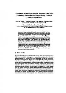
1. INTRODUCTION An important field of application of 3D scene analysis concerns sport games. The SIMULFOOT project started two years ago within the frame of the IFR Marey, a new organization in Marseilles dedicated to Biomedical Gesture Analysis [1],[2]. Our main objective was to provide a technological platform to cognitive scientists so that they could investigate in new theories about group be-haviors and individual perceptions, and validate them [3],[4],[5],[6]. Another objective of this project was to apply it to practical cases in collaboration with sports partners such as soccer and basketball clubs. In order to select the 3D model elements and to register them in space, we need to define in the 2D image a Region of Interest in which these elements will be captured [7],[8],[9]. And we also need to determine landmarks that will be used to provide the 2D to 3D registration [10],[11],[12],[13]. Before providing any player detection and scene analysis, we need to select a Region of Interest in the image as illustrated in Figure 1. We do it by taking advantage first on color coherence and then on topology coherence.
Figure 1: The region of interest is bounded by the red line and contains points, in yellow, for the 2D to 3D registration process • Extracting the most relevant subset within the whole set of points (color coherence) • Selecting the corresponding points in the image • Defining the region of interest by applying an area coherence criterion on the selected pixels We will mainly focus on the color space segmentation that may be a very difficult task in some cases. The approach we propose in this paper is robust and can be applied to a wide set of situations. 2. A SURVEY OF VARIOUS APPROACHES FOR AUTOMATICALLY SELECTING A REGION OF INTEREST
The global process for selecting this Region of Interest consists in:
Many research works have been developed to automatically extract the foreground elements from the background in video sequences, such as the works described in [14] and [15]. But although it looks similar, the problem mentioned in this papers in completely different: we do not want to characterize the background but to find the area in the image that corresponds to the relevant part of the background.
• Analyzing the shape of the set of points representing all the pixels of the image in the color space
Concerning works on scene analysis related to team sports, we can mention an European initiative that lead to various
works, especially in the field of soccer scene analysis [16]. Let us also mention the works developed by Vandenbroucke on a method that provide a color space segmentation and classification before using snakes to track the players in video sequences [17]. The ideas developed in this paper are very interesting but they do not fully take advantage of the color and morphological coherence. Figure 3: Threshold on points occurence For these reason, we have developed a new approach that integrates all these features. 3. BASIC SEGMENTATION OF THE HLS SPACE All the pixels of a given image can be represented in a color space that is a 3D space. Usually, the information captured by a video camera is made of (red, green, blue) quantified values. But this color information can be represented in a more significant space such as the HLS (Hue, Lightness, Saturation) one, for example. We chose to work in the HLS space because it provides a direct access to the hue and this seems to be determinant for selecting the background color. The first idea we developed was to visualize all the points in the HLS space as illustrated in Figure 2.
Figure 2: One image and the corresponding set of points in HLS space But in fact, many problems arise when we want to use it directly in such a way. The first and main problem is that this representation is not very accurate. Because of color quantification many pixels have exactly the same RGB values and thus the same HLS ones: all these points are visualized as a single point and, consequently, it provides a wrong idea of the point distribution. It is then difficult to provide a pixel selection directly based on this representation. For example, in Figure 3, we only have selected pixels that occur at least 16 times and we can see that the result is not satisfactory. The reason is that many pixels can have very close values without occurring very often. These remarks inclined us to use a different approach to analyze the point distribution in the HLS space. We consider this space as a discrete one and we evaluate the con-
tribution of the points (representing the pixels) to each cell (volume element of the discrete HLS space). Then we keep the most significant cells to provide the selection. 4. A DISCRETE REPRESENTATION OF THE HLS COLOR SPACE We represent the HLS space as a set of volume elements each of them being defined by a set of constraints on the H, L and S values. We have chosen the following repartition that provides an interesting discrete model made of 554 cells in table 1(each line gives the number of intervals in H, in S and globally for each interval in L). Luminance [0.95,0.1] [0.9,0.95] [0.8,0.9] [0.7,0.8] [0.6,0.7] [0.5,0.6] [0.4,0.5] [0.3,0.4] [0.2,0.3] [0.1,0.2] [0.05,0.1]
Saturation 1 2 4 4 8 8 8 8 4 4 2
Hue 1 6 6 12 12 12 12 12 12 6 6
Cells 1 12 24 48 96 96 96 96 48 24 12
Table 1: HLS space discret model This HLS space discrete representation can be illustrated, for example, as a set of juxtaposed polyhedrons or as a set of small spheres centered in each polyhedron (Figure 4). This discretisation set the following neighborhood relations between the cells (Figure 5). Those relations are used both to compute accurately potential sources in the color space and to propagate it the discrete HLS space from cell to cell. By using this approach, we improve the initial selection but it still does not provide a full satisfactory result.
Figure 4: HLS space discrete representation
Figure 8:
Figure 9:
5. POTENTIAL SOURCES IN THE COLOR SPACE
Figure 5: the following neighborhood relations between the cells
In Figure 6 and 8, the two images show the decimation of this representation based on a threshold on the cell density. The green cell the most on the right (the most saturated) disappeared before the cells along luminance axis.
As we can see on the polyhedral representation, all the cells do not have the same size and thus, the potential incidence is not the same on all the parts of the discrete HLS space. In order to avoid such a default, we propose a variable range that depends on cell size and that is computed as follows. Let us consider R = D ÷ 2 where D is the diameter of the cell to which the point belongs (the diameter is the highest distance between two points of the cell). Then D M ax is evaluated as D M ax = R × (1 + ε) where ε represents the increasing percentage on R and has not to be a small value. Each pixel of the image produces a point that is considered as a potential source in the discrete HLS space. We use a very simple potential expression that is a linear one. Each point contribute to increase the density of a cell if its distance in the center of the zone is lower than Dmax. The weaker this distance is, the more the contribution is strong.
Figure 6:
Figure 7:
Figure 7 and 9 show the result of the selection based on the last threshold value and that this green cell corresponds with a part of region of interest. This is not satisfactory, because of the information loss and of the remaining noise. We can notice that only using a threshold on the density is not the best solution. The reason is that in this approach, we do not consider the interactions between cells and consequently, we do not fully take advantage of color coherence. In order to avoid it, we have decided to induce interactions through cells by considering that each point is a source of potential and by evaluating the generated potential at the center of each cell.
Figure 10 show the emissions area (in yellow with variable intensity) in which a point will contribute to increase the density. For example P1 has a stronger potential than P2 on the grayed zone while P3 has a null potential for this zone. Figure 11 and 13 show how potentiel sources improves the pixel selection through the color space: the cells along axis luminance can be eliminated by thresholding before some of the green ones that have a higher value thanks to the contributions of their neighbors (color coherence). 6. AUTOMATIC THRESHOLDING Up to now, we only considered a manual selection of the threshold value. Let us describe the classical but efficient algorithm we use to automatically select it.
Figure 13:
Figure 14:
Figure 10: Polyhedrons representing some of the cells
Table 2: Area density cumulated histogram Figure 11:
Figure 12: 7. USING AREA COHERENCE
Let us consider the distribution of the potential values in the 554 areas of the discrete HLS space. Most values are low ones and a few of them are high ones. We sort these values by decreasing order and we evaluate the function F that gives their cumulated value (i.e. F(1) is the highest potential, F(2) is the sum of the two highest potentials, and so on). This function starts at 0, it strongly varies on a few values and then it slowly varies to the value 554 of the variable. The breakpoint of the representative curve is significant of the threshold value. This breakpoint is obtained through the segmentation in two parts of the curve using a split and merge algorithm. We start from the area that has the highest density. Then, we look for other areas that are connected (neighborhood relations have been defined previously Figure 5) until we reach the number of areas determined through the analysis of the cumulated histogram (Table 2). The result is a set of areas in the discrete HLS space as represented below (Figure 15).
We now have to use the area coherence to definitively determine the Region of Interest. In the frame of the applications mentioned above, the 3D scene is characterized by a set of elements (usually the players) and a set of lines on the ground. The first ones produce holes in the Region of Interest and the second ones split it into different connected components. But these connected components are very close one to each other. First, we apply to this image a closing with a structuring element which size is over the usual line width: it provides the connection between all these connected components. Second, we apply to the result an opening with the slightly bigger structuring element in order to eliminate all the non-significant elements on the border of the Region of Interest. In the two previous paragraphs, the discussion was related to the Region of Interest but, in fact, it had not been found at this step of the algorithm. This area is simply obtained as the connected component (after the closing and the opening) that contains the most pixels.
Figure 15: set of automatically selected areas in the discrete HLS space Figure 17: A Rolland Garros picture The last step of this process consists in filling the holes of the Region of Interest by using a classical Area filling algorithm. Figure 16 shows the result of this process in the example that has been used all along this paper to illustrate our approach. After the closing and the opening we have highlighted the border of the Region of Interest finally detected.
Figure 18: The model of variable potential is more efficient
Figure 16: In Red, the region of interest
8. SOME RESULTS We illustrate the whole process on another example (Figure 17) that shows the variability of the approach proposed in this paper. This example deals with tennis: the color is different, the size and the location of the Region of Interest are different. In Figure 18, the following two images show the discrete HLS space with successively the density and the variable potential. It illustrates as well as in the previous example the improvements brought in the approach (the right image provides a reliable vision of the color distribution). Figure 19 shows the result of the threshold in the discrete HLS space and it application to the image. Finally, we obtain the following Region of Interest (Figure 20):
Figure 19: The automatically selected pixels
Figure 20: In Red, the region of interest
9. CONCLUSION The approach described in this paper has been developed in the frame of a project in which we can identify a specific background mainly through its color coherence. This approach is quite robust for this application. It could be interesting to develop it in a more general frame (for industrial vision, for instance) when various backgrounds are present in the image: this would imply, on the same basis, to analyze more precisely the shape of the so generated 3D potential in the discrete HLS space.
10. REFERENCES [1] S. Mavromatis, J. Baratgin, J. Sequeira, ”Reconstruction and simulation of soccer sequences,” MIRAGE 2003, Nice, France. [2] S. Mavromatis, J. Baratgin, J. Sequeira, ”Analyzing team sport strategies by means of graphical simulation,” ICISP 2003, June 2003, Agadir, Morroco. [3] H. Ripoll, ”Cognition and decision making in sport,” International Perspectives on Sport and Exercise Psychology, S. Serpa, J. Alves, and V. Pataco, Eds. Morgantown, WV: Fitness Information technology, Inc., 1994, pp. 70-77. [4] A. M. Williams, K. Davids, L. Burwitz, and J. G. Williams, ”Cognitive knowledge and soccer performance,” Perceptual and Motor Skills, vol. 76, pp. 579-593, 1993. [5] L. Saitta and J. D. Zucker, ”A model of abstraction in visual perception,” Applied Artificial Intelligence, vol. 15, pp. 761-776, 2001. [6] K. A. Ericsson and A. C. Lehmann, ”Expert and exceptional performance: Evidence of maximal adaptation to task constraints,” Annual Review of Psychology, vol. 47, pp. 273-305, 1996. [7] B. Bebie, ”Soccerman : reconstructing soccer games from video sequences,” presented at IEEE International Conference on Image Processing, Chicago, 1998. [8] M. Ohno, Shirai, ”Tracking players and estimation of the 3D position of a ball in soccer games,” presented at IAPR International Conference on Pattern Recognition, Barcelona, 2000. [9] C. Seo, Kim, Hong, ”Where are the ball and players ? : soccer game analysis with colorbased tracking and image mosaick,” presented at IAPR International Conference on Image Analysis and Processing, Florence, 1997. [10] S. Carvalho, Gattas, ”Image-based Modeling Using a Twostep Camera calibration Method,” presented at Proceedings of International Symposium on Computer Graphics, Image Processing and Vision, Rio de Janeiro, 1998. [11] L. Faugeras, Maybank, ”Camera SelfCalibration : Theory and Experiments,” presented at Proceedings of Computer Vision, Berlin, 1992.
[12] H. Liu, Faugeras, ”Determination of Camera Location from 2-D to 3-D Line and Point Correspondences,” IEEE Transaction on Pattern Analysis and Machine Intelligence, vol. 12, pp. 28-37, 1990. [13] Tsai, ”An Efficient and Accurate Camera Calibration Technique for 3D Machine Vision,” presented at IEEE Conference on Computer Vision and Pattern Recognition, Miami Beach, 1986. [14] A. Amer, A. Mitiche, E. Dubois, ”Context independent real-time event recognition: application to key-image extraction.” International Conference on Pattern Recognition Qubec (Canada) August 2002. [15] S. Lefvre, L. Mercier, V. Tiberghien, N. Vincent, ”Multiresolution color image segmentation applied to background extraction in outdoor images.” IST European Conference on Color in Graphics, Image and Vision, pp. 363367 Poitiers (France) April 2002. [16] Assavid, ”Automatic segmentation and semantic annotation of sports videos.” European Project of the 5th PCRD, IST-1999-13082 January 2000. [17] N. Vandenbroucke, L. Macaire, J. Postaire, ”Color pixels classification in an hybrid color space.” IEEE International conference on Image Processing, pp. 176-180 Chicago 1998.