Automatic Structure Detection for Popular Music Changsheng Xu1, Namunu C Maddage1,2, Mohan S Kankanhalli2 1 2 Institute for Infocomm Research School of Computing 21, Heng Mui Keng Terrace National University of Singapore Singapore 119613 Singapore 117543 {xucs, maddage}@i2r.a-star.edu.sg
[email protected]
ABSTRACT Music structure is very important for semantic music understanding. We propose a novel approach for popular music structure detection. The proposed approach applies beat space segmentation, chord detection, singing voice boundary detection, melody and content based similarity region detection to music structure detection. A frequency scaling “Octave Scale” is used to calculate Cepstral coefficients to represent the music content. The experiments illustrate that the proposed approach achieves better performance than existing methods. We also outline some applications which can use our refined music structural analysis. 1. INTRODUCTION Music structure information is important for music semantic understanding. Its components, e.g. Introduction (Intro), Verse, Chorus, Bridge, Instrumental and Ending (Outro), can be identified by determining the melody-based similarity regions and content-based similarity regions in a song. We define melody-based similarity regions as the regions that have similar pitch contours constructed from the chord patterns and content-based similarity regions as the regions which have both similar vocal content and similar melody. For example, the Verse sections in a song can be considered as melodybased similarity regions while Chorus sections are content-based similarity regions. There are some earlier works on music structure analysis. Cooper [4] analyzed how rhythm is perceived and established in mind. Narmour [24] proposed a theory of cognition of melodies based on a set of basic grouping structures which characterize patterns of melody implications that constitute the basic units of the listener’s perception. Lerdahl [17] proposed a Generative Theory of Tonal Music. According to this theory, music is built from an inventory of notes and a set of rules. These rules assemble notes into a sequence and organize them into a hierarchical structure of music cognition. Dennenberg [7] proposed chroma-based and autocorrelation-based techniques to detect the melody line in the music. Repeated segments in the music are identified using Euclidean distance similarity matching and clustering of the music segments. Goto [13] and Bartsch [1] constructed vectors from extracted pitch sensitive chroma-based features and measured the similarities between these vectors to find the repeating sections (i.e- chorus) of the music. Foote and Cooper [10] extracted mel-frequency cepstral coefficients (MFCC) and constructed similarity matrix to compute the most salient sections in the music. Cooper [8] extracted MFCCs from the music content and reduced the vector dimensions using singular value decomposition techniques. Then global similarity function was defined to find the most salient music section. Logan [1] used clustering and hidden Markov model (HMM) to detect the key phrases which were considered to be the most repetitive sections in the song. For automatic music summarization, Lu [19] extracted octave-based spectral contrast and MFCCs to characterize the music signals and the most salient segment of the music was detected based on its occurrence frequency. Then the music signal was filtered using the band pass filter in the (125 ~1000) Hz frequency range to find the
music phrase boundary. These boundaries were used to ensure that an extracted summary did not break the music phrase. Xu [32] analyzed the signal in both time and frequency domains using linear prediction coefficients (LPC) and MFCCs. An adaptive clustering method was introduced to find the salient sections in the music. Chai [2] generated music thumbnails by representing music signals with pitch, spectral and chroma-based features and then matching their similarities using dynamic programming. The limitation of above-mentioned methods is that most of the methods have not exploited music domain knowledge and addressed the following issues of the music structure analysis: • The estimation of the boundaries of repeating sections is difficult if time signature (TS)1, meter (M)2 and Key3 of the song are unknown. •
In some song structures, Chorus and different Verses either have the same melody (pitch contour) or tone/semitone shifted melody (different music scale). In such cases, it is not guaranteed that we can correctly identify the verse and chorus without analyzing the vocal content of the music.
In this article we introduce a novel approach, which combines both high-level music structure knowledge and low-level audio signal processing techniques, to define the music structure via the detection both melody-based and content-based similarity regions. Part of the work was published in [20]. The content-based similarity regions in the music are important for many applications such as music summarization, music transcription, automatic lyrics recognition, music information retrieval, and music streaming. Figure 1 shows how our proposed approach works for music structure detection. 1. Firstly the rhythm structure of the music is analyzed by detecting note onsets and the beats. The music is segmented into frames with the size of inter-beat time length. We call this segmentation method as beat space segmentation. 2. Secondly, a statistical learning method is used to identify the melody transition via detection of chord patterns (section 4) in the music and detect singing voice boundaries. 3. Finally, with the help of repeated chord pattern analysis and vocal content analysis, the music structure is detected. Chord detection
1. Rhythm extraction Song
Music knowledge
2. Beat space segmentation 3. Silence detection
Singing voice boundary detection
Music structure detection
Figure 1: Music structure detection The rest of the article is organized as follows. In section 2, we introduce the music theory and song structure which will be used for music structure analysis in this article. Beat space segmentation, chord detection, singing voice boundary detection, and music structure analysis are described in section 3, 4, 5, and 6 respectively. Experimental results are reported in section 7. Some applications are discussed in section 8. We conclude the paper with future work in section 9. 1
Number of beats per bar; TS 4/4 implies four crotchet beats in the bar ( sect 2.1)
2
Number of beats per minutes; if the TS is 4/4 then meter (M) indicates how many crotchet beats per minutes.
3
Set of chords by which the piece is built. (sect 2.2)
2. MUSIC KNOWLEDGE From the music composition point of view, all the measures of music event changes in the music are based on the discrete step size of music notes. Section 2.1 introduces time alignments between music notes and phrases. This information is directly embedded with the music segmentation discussed in section 3. Music chords, key, and scale described in section 2.2 reveal how such information can be used to correctly measure melody fluctuations in a song (See section 4). General composition knowledge used for song writing is discussed in section 2.3 and has been incorporated in section 6 for high level music structure formulation. 2.1 Music notes The note duration is characterized by onset and offset times of a note. The correlation of music notes length, symbols, identities and their relationships with the silences (rest) are shown in Figure 2. The duration of a song is measured as number of Bars [26]. While listening to music, the steady throb to which one could clap is called the Pulse or the Beat and the Accents are the beats which are stronger than the others. The numbers of beats from one accent to adjacent accents are equal and it divides the music into equal measure. Thus, the equal measure of number of beats from one accent to another is called the bar. The time signature (TS) is defined as the number of beats per bar. The most common TS in popular music is four crotchet beats in a bar, written as 4/4. Note
Shape
Semibreve Minim Crotchet Quaver Semiquaver Demisemiquaver
Rest
or
Value in terms of Corresponding names generally used in U.S.A and Canada a Semibreve 1 Whole Note Half Note 1/2 Quarter Note 1/4 1/8 Eighth Note 1/16 Sixteenth Note Thirty-second Note 1/32
Figure 2: Correlation between different music notes and their time alignment In a song, the words or syllables in the sentence fall on beats in order to construct a music phrase. Figure 3 illustrates how words ‘Baa, baa, black sheep, have you any wool?’ form themselves into a rhythm and its music notation. The 1st and 2nd bars are formed with two quarter notes each. Four eighth notes and a half note are placed in the 3rd and 4th bars respectively to sound the words rhythmically.
2/4 ‘Baa
baa,
black Sheep, have you
any
wool?’
Figure 3: Rhythmic groups of words A music phrase is commonly two or four bars in length. The incomplete bars are filled with notes or rests or humming (duration of humming is equal to the length of a music note). 2.2 Music scale, chords and key of a piece The eight basic notes (C, D, E, F, G, A, B, C), which are the white notes on the keyboard, can be arranged in an alphabetical succession of sounds ascending or descending from starting note. This note arrangement is known as music Scale. Figure 4(left) shows the note progression in G scale. In a music scale, the pitch progression of one note to the other is either half step (a Semitone-S) or the whole step (a Tone –T). Thus it expands the eight basic notes into 12 pitch classes. The first note in the scale is known as Tonic and it is the key-note (tone-note) from which the scale takes the name. Depending on
the pitch progression pattern, music scale is divided into one Major scale and three minor scales (Natural, Harmonic and Melodic). The Major scale and Natural Minor scale follow pattern of “T-T-S-TT-T-S” and “T-S-T-T-S-T-T” respectively. The table in Figure 4 lists the notes that are present in Major and Minor scales for the C pitch class. C
B
C# D
A#
D#
A
E
G# G
F#
F
G A B C D E F G G Scale
Figure 4: Succession of musical notes and music Scale Music chords are constructed by selecting notes from the corresponding scales. Types of chords are Major, Minor, Diminished and Augmented. The 1st note of the chord is the key–note in the scale and Table 1 shows the note distances to the 2nd, 3rd, and 4th notes of the chord from the key note. Table 1: Distance to the notes in the chord from the key note in the scale
T - Implies a Tone / Whole step in music theory
The possible set of chords which represent the Major and Minor of C scale are shown in Table 2. The set of notes on which the piece is built is known as the Key. Major key (the chords that can be derived from major scale) and Minor key (the chords that can be derived from three minor scales) are two possible kinds of keys in a scale. Table 2: Chords which comprise both C Major and Minor keys
2.3 Popular song structure The popular music structure often contains Intro, Verse, Chorus, Bridge, Middle eight and Outro [30]. The intro may be 2, 4, 8 or 16 bars long or there is perhaps no intro in a song. The intro is usually instrumental music. Both verse and chorus are 8 or 16 bars long. Typically the verse is not melodically as strong as the chorus but in some songs they are equally strong and most of the people can hum or sing their way. The gap between the verse and chorus is linked by a bridge which may be only 2 or 4 bars. Silence may act as a bridge between verse and chorus of a song, but such cases are rare. Middle eight which is 4 or 16 bars long, is an alternative version of verse with new chord progression possibly modulated with different key. It appears after the 3rd verse in the song. Many people use the term ‘middle eight’ and ‘bridge’ synonymously. However the main difference is that the middle eight is longer (usually 16 bars) than the bridge and it mostly appears after the 3rd verse in the song. There are instrumental sections in the song and they can be instrumental versions of chorus or verse or entirely different tunes with set of chords together. Outro is fade–outs of the last phrases of chorus. The above described parts of the song are commonly arranged simply verse-chorus and repeated pattern. Two variations on the themes are listed below: •
Intro, Verse 1, Chorus, Verse 2, Chorus, Chorus, Outro
•
Intro, Verse 1, Verse 2, Chorus, Verse 3, Middle eight, Chorus, Chorus, Outro
From the signal processing point of view, the above music theory information about the song structure reveals that the fluctuations of temporal properties (pitch/melody) of the music are proportional to beat time intervals. Thus in our proposed segmentation approach, we segment the music according to interbeat time length proportional frames instead of the conventional fixed-length segmentation in speech processing, where the beat length may be multiples of the note length. The calculation of inter-beat proportional frame length is explained in the next section. This beat space segmentation is primarily utilized for chord detection and singing voice boundary detection in a song. Furthermore, this rhythmbased music segmentation leads to both melody-based and content-based similarity region detection. 3. RHYTHM EXTRACTRION AND BEAT SPACE SEGMENTATION As explained in the previous section, the melody transition, music phases, semantic events (verse, chorus, etc) occur in inter-beat time proportional intervals. Here we narrow down our scope to English songs with 4/4 time signature which implies 4 quarter notes per bar and the commonly used meter [27]. In music composition smaller notes such as eighth, sixteenth or thirty-second notes are played along with music phrases to align instrumental melody with vocal pitch contours. Therefore, in our proposed music segmentation approach, we segment the music into the smallest note length frames. This is called beat space segmentation (BSS). To the best of our knowledge, we are the first to propose the idea of beat space segmentation for music analysis which was inspired from our proposed correction algorithm for music sequence (CAMS) in [21]. There is no similar automated approach done in the past. To calculate the duration of the smallest note, we first detect the note onsets and beats of the song according to the steps described in Figure 5.
Sub-band 8
Inter beat time length
Energy Transient
Dynamic Programing
Audio music
Onset detection
Frequency Transients
Moving Threshold
Sub-band 2
Quarter note length estimation using autocorrelation
Peak Tracking
Sub-band 1
Octave scale sub-band decomposition using Wavelets
Sub-string estimation and matching
Figure 5: Rhythm tracking and extraction Since the harmonics structure of music signals are in octaves (Figure 8), we decompose the music signal into 8 sub-bands whose frequency ranges are shown in Table 3. The sub-band signals are segmented into 60ms intervals with 50% overlapping and both the frequency and energy transients are analyzed using a method similar method to that in [9]. Both the fundamentals and harmonics of music notes in the popular music are strong in sub-band 01 to 04. Thus we measure the frequency transients in terms of progressive distances between the spectrums in these sub-bands. To reduce the effect of strong frequencies generated from percussion instruments and bass clef music notes (usually generated by base guitar and piano), the spectrums computed from the sub-band 03 and 04 are locally normalized before measuring the distances between the spectrums. The energy transients are computed for sub-band 05 to 08. Table 3: Fundamental frequencies (F0) of music notes and their placement in the octave scale sub-bands
In order to detect hard (bass clef) and soft (treble clef) onsets, we take the weighted sum of onsets, detected in each sub-band. In our experiments, it is noticed that hard onsets generated from bass drums, bass guitar and bass notes of piano can be found in sub-band 01 and 02. The timing of snares and side drums are highlighted in sub-band 07 and 08. These onsets can indicate the bar timing. The soft onsets are noticeable in sub-band 03 to 06. Music theories describe metrical structure as an alternation of strong and weak beats over time [16]. Both strong and weak beats indicate the bar and note level time information respectively. We take weighted summation over sub-bands’ onsets to find the final series of onsets. The initial inter-beat length is estimated by taking the autocorrelation over the detected onsets.
(a) Strength
We employ a dynamic programming approach to check for patterns of equally spaced strong and weak beats among the computed onsets. Since our main purpose of onset detection is to calculate the interbeat timing and note level timing, it is not necessary to detect all the onsets in the song. Figure 6(a) shows a 10 second clip of “Still the One-Shania Twain”. The detected onsets are shown in Figure 6(b). The autocorrelation over detected onsets is shown in Figure 6(c). Both the sixteenth note level segmentation and bar measure are shown in Figure 6(d). 10 second clip from “Still The One - Shania Twain”
1 0.5 0 -0.5 -1
(c) Energy
(b) Strength
0 1.00 0.75 0.50 0.25 0
1
1.5
2 Detected onsets
2.5
3
3.5
4
x 105
0.5
1
1.5
2
2.5
3
3.5
4
x 105
2.5
3
3.5
4
x 105
2.5
3
3.5
4
x 105
4 3 2 1
Results of autocorrelation
0 (d) Strength
0.5
0.5
1.0
1
1.5
2
25th bar
27th bar
0.5 0
0.5
1
1.5
2
Sample number (sampling frequency = 44100 Hz)
Figure 6: (44.39 ~54.39) seconds clip of the song “Still the One-sung by Shania Twain”. Sixteenth note length is 112.10625ms. After BSS, we need to detect the silence frames and remove them. Silence is defined as a segment of imperceptible music, including unnoticeable noise and very short clicks. We use short-time energy function to detect the silent frames, where w(m), the rectangular window length, is equal to inter-beat time length. The short-time energy function of a music signal is defined as En =
1 ∑ [ x( m) w(n − m)]2 N m
(1)
where x(m) is the discrete time music signal, n is time index of the short-time energy, and w(m) is a rectangle window, i.e. 0 ≤ n ≤ N − 1, ⎧1, (2) w(n) = ⎨ ⎩0,
otherwise.
The non-silence beat space segmented frames are further analyzed for chord detection (section 4) and singing voice boundary detection (section 5).
4. CHORD DETECTION A chord, as described in section 2.2, is constructed by playing 3 or 4 music notes simultaneously. Thus detecting the fundamental frequencies (F0s) of notes which comprise chord is the key idea to identify the chord. Chord detection is essential to identify melody-based similarity regions which have similar chord pattern. The vocal content in these regions may be different, but envelops of chord sequences corresponding to verse and chorus sections are similar. Therefore, in some songs, both verse and chorus have a similar melody. We use a similar method described in [28] for chord detection. The Pitch Class Profile (PCP) features, which are highly sensitive to the F0s of notes, are extracted from training samples to model the chord with HMM. The polyphonic music contains signals of different music notes played at lower and higher octaves. Some music instruments such as string type instruments have the strong 3rd harmonic component [25] which nearly overlaps with the 8th semitone of next high octave. This will lead to wrong chord detection. For example, the 3rd harmonic of note C in (C3 ~ B3) and F0 of note G in (C4 ~ B4) are nearly overlap (see Table 3). To overcome this, in our implementation beat space segmented frames are represented in frequency domain with 2Hz frequency resolution using short-time Fourier transform (STFT). Then the linear frequency is mapped into the octave scale, where the pitch of each semitone is represented with as high resolution as 100 cents4. We consider 128~8192Hz frequency range (sub-band 02 ~ 07 in Table 3) to construct the PCP feature vectors to avoid percussion noise, i.e. base drums in lower frequencies below 128 Hz and both cymbal and snare drums in higher frequencies over 8192Hz, to be added to PCP features. We use 48 HMMs to model 12 Major, 12 Minor, 12 Diminished and 12 augmented chords. Each model has 5 states including entry and exit and 3 Gaussian Mixtures (GM) for each hidden state. The mixture weights, means and covariance of all GMs and initial and transition state probabilities are computed using Baum-Welch algorithm [33]. Then the Viterbi algorithm [33] is applied to find the efficient path from starting to end state in the models. It can be seen from Table 1, that the pitch difference between the notes of chord pairs is small. In our experiments, sometimes we find that observed final state probabilities of HMMs corresponding to these chord pairs are high and close to each other. This may lead to wrong chord detection. Thus we apply rule-based method (key determination) to correct the detected chords and apply heuristic rules based on popular music composition to further correct the time alignment (chord transition) of the chords. Song writers use relative Major and Minor key combinations in different sections, perhaps minor key for Middle eight and major key for the rest, which would break up the perceptual monotony effect of the song. Therefore a 16-bar length with 14 bars overlap window is run over the detected chords to determine the key of that section. The majority of chords that belongs to a key is assigned as the key of that section. The 16-bar length window is sufficient to identify the key [29]. If Middle eight is present, we can estimate the region where it appears in the song by detecting the key change. Once the key is determined, the error chord is corrected as follow: •
Normalize the observations of the 48 HMMs which represent 48 chords according to the highest probability observed from the error chord.
•
If the observation is above a certain threshold and it is the highest observation among all chords in a key, the error chord is replaced by the next highest observed chord which belongs to the same key.
•
If there are no observations belonging to the key above the threshold, assign the previous chord.
4
It is a logarithmic measure of relative pitch or intervals [22].
The music signal can be considered as quasi-stationary between the inter-beat times, because the melody transition occurs on beat time. Thus we apply the following chord knowledge [14] to correct the chord transition within the window. 1. Chords are more likely to change on beat times than on other positions. 2. Chords are more likely to change on half note times than on other positions of beat times. 3. Chords are more likely to change at the beginning of the measures (bars) than at other positions of half note times. The above 3 points are explained in Figure 7. In Figure 7, the size of the beat space segment is eighth notes and the size of the half note is 4 beat space segments. After the correction, bar i has 2 chord transitions and a chord in bar (i+1). Size of the beat space segment = 8th note length Chords
Time signature 4/4 Bar i
Bar (i+1)
Detected chords sequence Corrected chord sequence
Half a note length
Figure 7: Correction of chord transition 5. SINGING VOICE BOUNDARY DETECTION For the similar melodies in the choruses, they may have different instrumental setup to break the perceptual monotony effect in the song. For example, the 1st chorus may contain snare drums with piano music and the 2nd chorus may progress with bass and snare drums with rhythm guitar. After detecting melody-based similarity regions, it is important to decide which regions have similar vocal contents. Therefore, singing voice boundary detection is the first step to analyze the vocal content. In the previous works related to singing voice detection, Berenzweig et al. [2] used probabilistic features calculated by Cepstral coefficients to train HMM to classify vocal and instrumental music. Kim et al. [15] used an IIR filter and an inverse comb filter bank to detect the vocal boundaries. Zhang [34] used a simple threshold calculated using energy, average zero crossing, harmonic coefficients and spectral flux features to find the starting point of the vocal part. For instrument identification, Fujinaga [11] trained a K-nearest neighbor classifier with features extracted from 1338 spectral slices representing 23 instruments playing a range of pitches. However none of these methods has utilized music knowledge. In our method we further analyze the beat space segmented frames to detect the vocal and instrumental frames. Figure 8 (top) illustrates (a) the log spectrums of beat space segmented piano mixed vocals, (b) mouth organ instrumental music, and (c) log spectrum of fixed length speech. The analysis of harmonic structures indicates that the frequency components in (a) and (b) spectrums are enveloped in octaves. Figure 8 (bottom) illustrates the ideal octave scale spectral envelops. Since the instrumental signals are wide band signals (up to 15 kHz), the octave spectral envelops in instrumental signals are wider than those in vocal signals. However the similar spectral envelops cannot be seen in the spectrum of speech signal.
(b)
2 0
16000 18000
6000
0
8192
4096
2048
1024
256 512
(c)
Frequency (Hz)
Log magnitude of the spectrum envelops
0
8000 10000 12000
-4 Log spectrum of beat space segment -6 0 2000 4000
9000
7000 8000
2000
0
3000 4000 5000 6000
(a)
14000
-2
Log spectrum of 600ms segment
8000 9000
4
6 4 2 0 -2 -4 -6 -8
4000 5000 6000 7000
6
1000 2000 3000
Log spectrum of beat space segment
1000
Log magnitude
8 6 4 2 0 -2 -4 -6
(Hz)
Octaves scale frequency spacing
Figure 8: Top figures, (a) - Quarter note length (662ms) guitar mixed vocal music; (b) – Quarter note length (662ms) instrumental music (mouth organ); (c) - Fixed length (600ms) speech signal. Bottom figure – Ideal octave scale spectral envelop. Thus we use a frequency scaling method called the “Octave Scale” instead of the Mel scale to calculate Cepstral coefficients [8] to represent the music content. The fundamental frequencies F0 and the harmonic structures of music notes in octave scale are shown in Table 3. Sung vocal lines always follow the instrumental line such that both pitch and harmonic structure variations are also in octave scale. In our approach we divide the whole frequency band into 8 sub-bands (the first row in Table 3) corresponding to the Octaves in music. The useful range of fundamental frequencies of tones produced by music instruments is considerably less than the audible frequency range. The highest tone of the piano has a frequency of 4186 Hz and this seems to have evolved as a practical upper limit for fundamental frequencies. We have considered the entire audible spectrum to accommodate the harmonics (overtones) of the high tones. The range of fundamental frequency of the voice demanded in classical opera is from ~80-1200 Hz corresponding to the low end of the bass voice and the high end of the soprano voice respectively. Table 4 shows the number of triangular filters which are octal spaced in each sub-band and empirically found to be good for identifying vocal and instrumental frames. It can be seen that the number of filters are maximum in the bands where the majority of the singing voice is present for better resolution of the signal in that range. Table 4: Number of filters linearly spaced in sub-bands Sub-band no
01
02 03 04 05 06 07 08
Number of filters
6
8
12 12 8
8
6
4
Cepstral coefficients are then extracted from the Octave Scale to characterize music content [8]. These Cepstral coefficients are called Octave Scale Cepstral coefficients (OSCCs). Singular values indicate the variance of the corresponding structure. Comparatively high singular values describe the number of dimension which the structure can be represented orthogonally, while smaller singular values indicate the correlated information in the structure. When the structure changes, these singular values also vary accordingly. However it is found that singular value variation is smaller in OSCCs than in MFCCs for both pure vocal music and vocal mixed instrumental music which implies OSCCs are more sensitive to vocals than vocal mixed instrumental music.
Singular value decomposition is applied to find the uncorrelated Cepstral coefficients for Octave scale. We use the order range of 10-16 coefficients for Octave scale. Then we train support vector machine to identify the pure instrumental (PI) and instrumental mixed vocal (IMV) frames. Our earlier experimental results [32] have shown that radial based kernel function Eq.(3) with c= 0.65, performs better in vocal/instrumental boundary detection. K ( x, y ) = exp( − x − y 2 c )
(3)
6. MUSIC STRUCTURE DETECTION We extract the high level music structure based on melody-based similarity regions detected according to chord transition patterns (section 4) and content-based similarity regions detected according to singing voice boundaries (section 5). Detection of melody-based and content-based similarity regions in the music are explained in section 6.1 and 6.2 respectively. Then we apply the music composition knowledge to detect the music structure. 6.1 Melody-based similarity region detection The repeating chord patterns form the melody-based similarity regions. We employ sub-chord pattern matching technique using dynamic programming to find the melody-based similarity regions (Figure 9). In Figure 9, regions R2, …, Ri, …., Rj have the same chord pattern (similar melody) as R1. Since it is difficult to detect all the chords correctly, the matching cost is not zero. Thus we normalized the costs and set a threshold (THcost) to find the local matching points closer to zero (Figure 10). THcost =0.3825 gives good results in our experiments. By counting the same number of frames as in the sub-pattern backward from the matching point we can detect the melody-based similarity regions. Matching point
R2
R3
Ri
Rj
Main chord pattern or sequence
R1 Sub chord pattern
Melody similarity regions based on chord pattern of R 1
Figure 9: Melody based similarity region matching by dynamic programming Figure 10 illustrates the matching of both 8 and 16 bar length chord pattern extracted from the beginning of the Verse 1 in the “Twenty Five Minutes by MLTR” song. Y-axis is the normalized cost of matching the pattern and X- axis is the frame number. We set the threshold THcost and analyze the matching cost below the threshold to find the pattern matching points in the song. The 8-bar length regions (R2 ~R3) have the same chord pattern as the 1st 8-bar chord pattern (R1) in Verse 1. When the matching pattern was extended to 16 bars (i.e. r1 region), we are not able to find a 16-bar length region which has the same chord pattern as the r1 region.
8 bar length sub chord pattern matching 16 bar length sub chord pattern matching Matching threshold (THcost) line for 8 bar length sub chord pattern 1
16 bar length 8 bar length
Cost
0.8 0.6 0.4 0.2
R1
R2 R3
r1 0
128
256
Starting point of the verse 1
384
512
640 768 Frame number
896
1024
1152
1280
1397
Figure 10: Both 8 and 16 bar length chord patterns match in the song “Twenty Five Minutes - MLTR” 6.2 Content-based similarity region detection For melody-based similarity regions Ri and Rj in Figure 9, we use the following steps to further analyze them for content-based similarity region detection. Step1: The beat space segmented vocal frames of two regions are first sub-segmented into 30 ms with 50% overlapping. Although two choruses have similar vocal content, they may have same melody with different set of instrumental setup. Therefore, we extract 20 coefficients of octave scale cepstral coefficient (OSCC) feature per frame as OSCCs are highly sensitive to vocal content and not to the instrumental melody changes. Figure 11 illustrates SVD analysis of the OSCCs and MFCCs extracted from both solo male track and guitar mixed male vocals of a SriLankan song “Ma bala Kale ( )”. The quarter note length is 662ms and the sub-frame size is 30ms with 50% overlap. Singular value variation of 20 OSCCs and 20 MFCCs for both pure vocals and vocal mixed with guitar are shown in Figure 11(a), (b), (d) and (e) respectively. The percentage variation of the singular values of each OSCC and MFCC when guitar music is mixed with respect to their values for solo vocals are shown in Figure 11(c) and (f) respectively. When whole 20 coefficients are considered, the average singular value variation for OSCC and MFCC are 17.18% and 34.35% respectively. When the first 10 coefficients are considered, they are 18.16% and 34.25% respectively. It can be concluded that even when the guitar music is mixed with vocals, the variation of OSCCs is much lower than the variation of MFCCs. Thus compared with MFCCs, OSCCs are more sensitive to the vocal line than to the instrumental music.
(a)
0.5
0.1 0
0.05 0
5
5
10
10
15
15
20
20
0.2 1
0.15 0.1
(b)
0
40
0.5
Male vocals with guitar music
0
5
5
10
10
15
15
5
10
15
20
Coefficient number
1
(d)
Male vocals
0.5
0.1 0
0.05 0
5
5
10
10
0.2
15
15
20
20
1
0.15
(e)
0.5
0.1
0
20
(c)
0.15
Male vocals with guitar music
0
0.05
20
20
0
Normalized strength of singular values derived from 20 MFCCs
Male vocals
0.15
0.05
Singular value variation in percentage (%)
0.2
1
Singular value variation in percentage (%)
Normalized strength of singular values derived from 20 OSCCs
0.2
5
5
10
15
20
10
15
20
10
15
20
(f) 40
20
0
5
Coefficient number
Figure 11: Analysis of SVD for OSCCs and MFCCs Step 2: The distance and dissimilarity between feature vectors of Ri and Rj are calculated using Eq. (4) and Eq. (5) respectively. The dissimilarity (Ri Rj) gives low value for the content-based similarity region pairs. dist Ri R j ( k ) =
Vi ( k ) − V j ( k ) Vi ( k ) * V j ( k )
i≠ j
distRi R j (k ) k =1 n
(4)
n
dissimilarity( Ri , R j ) = ∑
(5)
Step 3: To overcome the pattern matching errors due to detected error chords, we shift the regions back and forth by 4 bars with 2 bars overlap and repeat step 1 and step 2 to find the positions of the regions which give the minimum value for “dissimilarity (Ri Rj)”. Step 4: Calculate “dissimilarity (Ri Rj)” in all region pairs and normalize them. By setting a threshold (THsmlr), the region pairs below the THsmlr are detected as content-based similarity regions. This indicates that they belong to chorus regions. Based on our experiments, a value of THsmlr = 0.389 works well. Figure 12 illustrates the content-based similarity region detection based on melody-based similarity region pairs.
Melody similarity region i
Vi
{20-OSCCs}
Vocal Beat space segments (BSS)
Melody similarity region j
Vocal Sub frames 30ms 50% overlap
V (k ) - V (k ) i j
dist (k ) = Ri Rj V (k ) * V (k ) i j
Vj i ≠
{20-OSCCs}
j
n distRi Rj ( k ) dissimilarity ( R i , R j ) = ∑ n k=1
Figure 12: Content-based similarity region detection 6.3 Structure detection We apply following heuristics, which agree with most of the English songs, to detect music structure. cThe typical song structure follows the verse–chorus pattern repetition [30] as shown below. a. Intro, Verse 1, Chorus, Verse 2, Chorus, Chorus, Outro b. Intro, Verse 1, Verse 2, Chorus, Verse 3, Chorus, Middle eight or Bridge, Chorus, Chorus, Outro c. Intro, Verse 1, Verse 2, Chorus, Verse 3, Middle eight or Bridge, Chorus, Chorus, Outro dThe minimum number of verse and chorus is 2 and 3 respectively. eThe verse and chorus are 8 or 16 bars long. fThe middle eight is 8 or 16 bars long. It has either the main key of a song or different keys. If the length of Middle eight is less than 8 bars it is identified as a bridge. The set of notes on which the piece is built is defined as the key. For example, C major key is derived from the chords in the C major scale. Based on our dataset, which only includes English songs, the statement of "songs with multiple keys are rare" is true. But if this is extended to other language songs (e.g. Japanese songs), such statement may not be true. Therefore, we now avoid giving a false impression of generality by explicitly stating that the techniques and results presented in the paper apply only to English pop songs. 6.3.1 Intro detection According to the song structure, Intro section is located before Verse 1. Thus we extract the instrumental section till the 1st vocal frame and detect this section as Intro. If silent frames are detected at the beginning of the song, they are not considered as part of intro because they do not carry a melody. 6.3.2 Verses and Chorus detection Since the end of the Intro is the beginning of Verse 1, we assume the length of Verse 1 is 8 or 16 bars and use this length chord sequence to find the melody-based similarity regions in a song. If there are only 2 or 3 melody-based similarity regions, they are the verses. Thus it can be concluded that the chorus does not have same chord pattern as the verses. Case 1 and Case 2 explain the detection of choruses and verses.
Case 1: Two melody-based similarity regions are found In this case, the song has the structure described in (ca). If the gap between verse 1 & 2 is equal and more than 24 bars, both verse and chorus are 16 bars long each. If the gap is less than 16 bars, both verse and chorus are 8 bars long. Using the chord pattern of the first chorus between verse 1 & 2, we can detect other chorus regions according to section 6.1. Since a bridge may appear between verse and chorus or vice versa, we align the chorus by comparing the vocal similarities of the detected chorus regions according to section 6.2. Case 2: Three melody similarity regions are found. In this case, the song follows either the (cb) or the (cc) pattern. Thus the first chorus appears between verse 2 & 3 and we can find other chorus sections using similar procedure described in Case 1. If there are more than 3 melody-based similarity regions (j > 3 in Figure 9), it implies that chorus chord pattern is partially or fully similar to the verse chord pattern. Thus we detect the 8-bar length chorus sections (may not be the full length of the chorus) by analyzing the vocal similarities in the melodybased similarity regions. Case 3 and Case 4 illustrate the detection of verse and chorus. Case 3: If R2 (Figure 9) is found to be a part of chorus, the song follows the (ca) pattern. If the gaps between R1 & R2 and R2 & R3 are more than 8 bars, the verse and chorus are 16 bars long. Thus we increase the sub-chord pattern length to 16 bars and detect the verse sections. After the verse sections are found, we can detect the chorus sections using similar way in Case 1. Case 4: If R2 is found to be a verse, the song follows the (cb) or (cc) pattern. Chorus appears after R2 regions. By checking the gaps between R1 & R2 and R2 & R3, the length of the verse and chorus is similar to Case 3. We can find the verse and chorus regions by applying similar procedure described in Case 3 and Case 1. 6.3.3 Instrumental sections (INST) detection The Instrumental section may have similar melody as the chorus or verse. Therefore, the melody-based similarity regions which have only instrumental music are detected as INSTs. However some INSTs have different melody. In this case, a window of 4 bars is utilized to find regions which have INSTs. 6.3.4 Bridge and Middle eighth detection The appearance of a bridge between verse and chorus can be detected by checking the gap between them. However if the longer gap (more than 4 bars) between choruses is only instrumental, it is considered as INST, otherwise it is detected as a bridge. The section which has different key is detected as a middle eighth. 6.3.5 Outro detection From the song patterns (ca, cb, & cc), it can be seen that before the Outro there is a chorus. Thus we detect the Outro based on the length between the end of the last chorus and the song. 7. EXPERIMENTAL RESULTS We use 50 popular English songs (10-MLTR, 10-Bryan Adams, 10-Westlife, 10-Backstreet Boys, 6Beatles and 4-Shania Twin) for the experiments in chord detection, singing voice boundary detection and music structure detection. All the songs that we have selected follow the structures described in section 6.3. The original keys and chord timing of the songs were obtained from the commercially available music sheets. All the songs are first sampled at 44.1 kHz with 16 bits per sample and stereo format from commercial music CDs.
Then we manually annotated the songs to identify the timing of vocal/instrumental boundaries, chord transitions and song structure in terms of beat space segmented units (number of frames). Figure 13 shows one example of a manually annotated song section explaining how the music phrases and the chords change with inter-beat length. This annotation describes the time information of Intro, Verse, Chorus, Instrumental, and Outro in terms of 272.977 ms length frames. The frame length is equal to the eighth note length and it is the smallest note length that can be found in the song. The beat space measures of vocal and instrumental parts in the respective phrases (middle column- lyrics) are described in left most columns and right most columns. Then the silence frames (rest notes), which may contain unnoticeable noise, are detected by the characteristic lower short time energies of the frames.
Figure 13: Manually annotated the intro and the verse 1 of the song “Cloud No 9 by Bryan Adams” 7.1 Chord detection We use the HTK toolbox [33] to model 48 chord types with HMMs. We use the first 35 songs (1 to 35) for training and the last 15 songs (36 to 50) for testing. Then we repeat the training and testing with different circular combinations such as song 16 to 50 for training and song 1 to 15 for testing. Since the number of training chord samples in the songs are not enough, the additional training data from the chord database is used for training. Thus we have over 10 minutes for each chord sample data for training each HMM. Our chord database consists of different sets of chords that are generated from original instruments (Piano, bass guitar, rhythm guitar etc), synthetic instruments (Roland RS- 70 synthesizer, cakewalk software), synthetically mixed instrumental notes by changing the time delay of the corresponding notes, and synthetically mixed male and female vocal notes (Doh, Ray, Me, Fah, Soh, Lah, Te, Doh). The recorded instrumental chords span from C3 to B6, comprising 4 octaves. The average frame-based accuracy of chord detection is 80.87%. We also are able to determine the correct key of all the songs. After error correction with key information, we can achieve 85.49% framebased accuracy. 7.2 Singing voice boundary detection The SVM Torch II [6] software package is used to classify frames into vocal or instrumental class. The support vectors (SV) are trained with 12 OSCCs extracted from each non-overlapping beat space segment. The radial based function (RBF) with c= 0.65 is used in the SVM kernel. The parameters used to tune OSCCs are the number of filter and their distribution in the octave frequency scale (section 5). 30 songs for SVM training and 20 songs for testing are employed with 4 different song combinations to evaluate the accuracy. Table 5 illustrates the comparison of the average frame-based classification
accuracy of OSCCs and MFCCs. It is empirically found that both the number of filters and coefficients of the feature give the best performance in classifying instrumental frames (PI- pure instrumental) and vocal frames (PV-Pure vocals, IMV- Instrumental mixed vocals). Table 5: Correct classification in percentage for vocal and instrumental classes Feature
No of filters
No of coefficients
PI
IMV+PV
OSCC
64
12
82.94
79.93
MFCC
36
24
75.56
74.81
We further apply music knowledge and heuristic rules [30] to correct the errors of misclassified vocal/instrument frames. Table 6 shows the comparison of the frame-based classification accuracies of SVM with and without rule-based error corrections. It can be seen that the classification accuracy can be significantly improved by 2.5 ~5.0% for both vocal and instrumental frames after applying rule-based error corrections. Table 6: Comparison of SVM with and without rules SVM
PI (%)
IMV+PV (%)
Without rules
82.94
79.93
With rules
86.02
84.55
7.3 Intro/verse/chorus/bridge/outro detection We use following two criteria to evaluate the result of detected music structure. ¾ The accuracy of all the parts in the music identified. For example, if 2/3 of the choruses are identified in a song, the accuracy of identifying the choruses is 66.66%. ¾ The accuracy of the sections detected. The detection accuracy of a section is illustrated in Eq. (6). For example, the detection accuracies of 3 chorus sections are 80.0%, 89.0% and 0.0%, the average detection accuracy of the chorus section is (80+ 89+0)/3 = 56. 33%. Detection accuracy ⎫ length of correctly detected section * 100 ⎬= of a section ( %) correct length ⎭
(6)
In Table 6, the accuracy of both identification and detection of the structural parts in the song “Twenty Five Minutes by MLTR” is reported. Since the song has 4 choruses and they are identified, 100% accuracy is achieved in identification of chorus sections in the song. However the average correct length detection accuracy of the chorus is 92.74%.
Table 6: Evaluation of both identified and detected parts in the song “Twenty Five Minutes by MLTR”
Song name: 25 minutes Parts in the song
Artist : MLTR I 1
Number of parts Number of parts identified
BSS length: 180.03ms BSS: 16th note O INST C B V ME 0 2 1 1 4 3 1 4 0 2 1 3
Individual accuracy of parts identification (in %)
1 100
100
100
100
100
Average detection accuracy (in %)
100
95.22
92.74
100
89.19
100
100
94.35 94.12
I - Intro, V - Verse, C - Chorus, B - Bridge, O - Outro ME - Middle Eighth
Figure 14 illustrates our experimental results for average accuracy detection of different sections. It can be seen that Intro (I) and the Outro (O) can be detected with very high accuracy. But detection accuracy for Bridge (B) sections is the lowest. % 100 95 90 85 80 75 70 65 60
Identification accuracy
100 96.22
86.51
84.29 77.48
Detection accuracy 90.78 80.18
79.16
Verse
Chorus
INTS
87.86 83.73
76.19
Inst
97.38 88.96
Bridge
71.48
Middle eightth
Outro
Figure 14: The average detection accuracies of different sections We compare our chorus detection method with an earlier method described in [13] using our testing dataset. Using previous method, reported identification accuracy and the detection accuracy are 67.83% and 70.18% respectively. 8. APPLICATIONS Music structure analysis can be used for many applications for music handling, such as music transcription, music summarization, music information retrieval, and music streaming, etc. 8.1 Music transcription and lyrics identification Both rhythm extraction and vocal/instrumental boundary detection are the preliminary steps towards lyrics identification and music transcription applications. Since music phrases are constructed with rhythmically spoken lyrics [26], rhythm analysis and beat space segmentation can be used to identify the word boundary in the polyphonic music signal. Together with signal separation techniques, it can reduce the complexity of identifying the voiced/unvoiced regions within the signal (see Figure 11) and lead the lyrics identification process simpler. In addition, the chord detection extracts the pitch/melody contour in the music and further analysis of beat space segmented music signals will help to estimate signal source mixture, which is the breaking point of music transcription. 8.2 Music summarization The creation of a concise and informative extraction that accurately summarizes original digital content is extremely important in large-scale information organization and processing. Nowadays, the most of music summaries used commercially are manually produced. So far a number of techniques have been proposed to automatically generating music summary [1],[32],[19],[2]. All these techniques are based on one assumption: the most repeated section of a song is the most memorable or distinguishable part.
Therefore, current approaches aiming at automatic music summarization focus on finding the most repeated section of the song using various methods. However, it is difficult to estimate both ends of the repeated sections. As a result, a summary will begin or end in the middle of music phrases, which will break the continuity of the music summarization and is not desirable for listeners. Based on successful music structure analysis, music summary can be generated more easily than the conventional methods. For example, from the music knowledge, the chorus sections are usually the most repeated sections in popular music. Therefore, if we can accurately detect the chorus in each song, we are likely to have also identified a good music summary. In addition, the difficulty of music phrase boundary detection can be solved nicely using proposed method because music phrases begin and end at the boundary of music bars. First the choruses are detected using proposed method. Since chorus happens more than once in a song, we can create music summary based on one of them. If the length of selected chorus is less than the desired length of final music summary, we can include the music phrases anterior or posterior to the selected chorus. To make the summary acceptable by listener, this music phrase should be intact which can be achieved by proposed rhythm analysis because music phrase in a song lasting a fixed number of music bars (Generally, 4, 6, or 8 bars for popular music). 8.3 Music information retrieval The ever increasing music collections require efficient and intuitive methods of searching and browsing. The music information retrieval (MIR) explores how music database may best be searched by providing input queries in some music form. For people who are not trained or educated with music theory, humming is the most natural way to formulate music queries. In most of MIR systems, a fundamental frequency tracking algorithm is used to parse a sung query for melody content [12]. The resulting melodic information is used to search a music database using either string matching techniques [23] or other models such as Hidden Markov Models [29]. However, a problem for query by humming is that the hummed melody can correspond to any part of the target melody (not just at the beginning), which makes it difficult to find the match starting point in the target melody. If we can detect the chorus accurately in a song, the location problem can be simpler. Because the choruses of the popular song are typically prominent and are generally sections that are readily recognized or remembered, the users are most likely to hum a fragment of chorus. Furthermore, since the chord sequences are a description that captures much of the character of a song, and the chord pattern changes periodically for a certain song, we can match the chords with our input humming, which will facilitate the retrieval process. 8.4 Music streaming Continuous media streaming over unreliable networks like Internet and wireless networks may encounter packet losses due to mismatch between the source coding and channel characteristics. The objective of the packet loss recovery in music streaming is to reconstruct a lost packet so that it is perceptually indistinguishable or sufficiently similar to the original one. The existing error concealment schemes [31], mainly employ either packet repetition techniques or signal restoration techniques. The most recently proposed content–based unequal error protection technique [31] effectively repairs the lost packets which have percussion signals. However this method is inefficient in repairing lost packets which contain signals other than percussion sounds (i.e. vocal signals and string, bowing & blowing types of instrumental signals). Therefore, the identification of music structure is necessarily needed to construct an efficient packet lost recovery scheme. For example, the instrumental/vocal boundary detection simplifies the signal content analysis at the sender’s end. Such analysis together with pitch information (melody contour) is helpful for better signal restoration at the receiver’s side. The contentbased similarity region identification can be construed to be a type of a music signal compression
scheme. Since structure analysis helps to identify content-based similarity regions such as chorus and instrumental music sections, we can avoid re-transmitting packets from similar regions and reduce the bandwidth consumption. Compared to the conventional audio compression technique such as MP3, which can attain a 5:1 compression ratio, using music structure analysis can potentially increase the compression ratio to 10:1. 9. CONCLUSION By combining high level music knowledge with existing audio processing techniques, we propose a robust semantic structural analysis approach for popular music. The experimental results illustrate that the proposed structural analysis method performs more accurately than existing methods. Looking at the results we conclude the following: 1. A combination of music knowledge with low-level audio processing is a powerful approach for performing music structure analysis. 2. Structural analysis is a vast topic, so we have narrowed down our scope to the music with 4/4 and chorus verse repetition. 3. Our approach aims to extract the basic ingredients of music structures that can immensely simplify the development of many applications. In fact, a colleague in the lab is looking at polyphonic content-based audio retrieval based on our structural analysis. The initial results are very promising. Based on the current work, we plan to extend the structure analysis to other music genres (e.g. classical, jazz) so as to come up with a generic music structure analysis approach. We also plan to explore more applications using the music structure information, such as music genre classification and digital music watermarking. 10. REFERENCES [1] Bartsch MA, Wakefield GH (2001) To Catch a Chorus: Using Chroma-based Representations for Audio Thumbnailing. In: Proceedings of the IEEE Workshop on Applications of Signal Processing to Audio and Acoustics, New Paltz, New York, USA, 21-24 October, 2001 [2] Berenzweig AL, Ellis DPW (2001) Location singing voice segments within music signals. In: Proceedings of the IEEE Workshop on Applications of Signal Processing to Audio and Acoustics, New Paltz, New York, USA, 21-24 October, 2001 [3] Chai W, Vercoe B (2003) Music Thumbnailing via Structural Analysis. In: Proceedings of ACM Multimedia, Berkeley, CA, USA, 2-8 November, 2003, pp 223-226 [4] Cooper G, Meyer LB (1960) The Rhythmic Structure of Music. The University of Chicago Press. 1960. [5] Cooper M, Foote J (2002) Automatic Music Summarization via Similarity Analysis. In: Proceeding of International Conference on Music Information Retrieval, Paris, France, 13-17 October, 2002 [6] Collobert R, Bengio S (2001) SVMTorch: Support Vector Machines for Large-Scale Regression Problems. In: Journal of Machine Learning Research, 2001, Vol 1, pp 143-160 [7] Dannenberg RB, Hu N (2002) Discovering Music Structure in Audio Recoding. In: Proceeding of 2nd International Conference on Music and Artificial Intelligence, Scotland, UK, 2002. pp 43-57. [8] Deller JR, Hansen JHL, Proakis HJG (1999) Discrete-Time Processing of Speech Signals. IEEE Press
[9] Duxburg C, Sandler M, Davies M (2002) A Hybrid Approach to Musical Note Onset Detection. In: Proceeding of International Conference on Digital Audio Effects, Hamburg, Germany, 26-28 September, 2002 [10] Foote J, Cooper M, Girgensohn A (2002) Creating Music Video using Automatic Media Analysis. In: Proceedings of ACM Multimedia, Juan-les-Pins, France, 01-06 December, 2002 [11] Fujinaga I (1998) Machine Recognition of Timbre Using Steady-state Tone of Acoustic Musical Instruments. In: Proceeding of International Music Conference, Michigan, USA, 01-06 October 1998, pp 207-210 [12] Ghias A, Logan J, Chamberlin D, and Smith BC (1995) Query By Humming: Musical Information Retrieval in an Audio Database. In: Proceedings of ACM Multimedia, San Francisco, CA, USA, 5-9 November, 1995, pp 231–236 [13] Goto MA (2003) Chorus-Section Detecting Method for Musical Audio Signals. In: Proceeding of the IEEE International Conference on Acoustics Speech and Signal Processing, Hong Kong, 6-10 April, 2003 [14] Goto M (2001) An Audio-based Real-time Beat Tracking System for Music With or Without Drumsounds. In: Journal of new Music Research, June 2001, Vol.30, No.2, pp 159-171 [15] Kim YK, Brian Y (2002) Singer Identification in Popular Music Recordings Using Voice Coding Features. In: Proceeding of International Conference on Music Information Retrieval, Paris, France, 13-17 October, 2002 [16] Large EW, Palmer C (2002) Perceive Temporal Regularity in Music. In: Journal of Cognitive Science, 2002, Vol 26, pp 1-37 [17] Lerdahl F, Jackendoff R (1983) A Generative Theory of Tonal Music. Cambridge: MIT Press. [18] Logan B, Chu S (2000) Music Summarization Using Key Phrases. In: Proceeding of the IEEE International Conference on Acoustics Speech and Signal Processing, Istanbul, Turkey, 05-09 June, 2000 [19] Lu L, Zhang H (2003) Automated Extraction of Music Snippets. In: Proceedings of ACM Multimedia, Berkeley, CA, USA, 2-8 November, 2003, pp 140-147 [20] Maddage NC, Xu CS, Kankanhalli MS, and Shao X (2004), Content-based Music Structure Analysis with Applications to Music Semantic Understanding, In: Proceedings of ACM Multimedia, New York, NY, USA, 11-16 October, 2004, pp 112-119 [21] Maddage NC, Xu CS, and Wang Y (2003), A SVM-Based Classification Approach to Musical Audio. In Proceedings of International Symposium of Music Information Retrieval (ISMIR), 2003. [22] Monzo JL (1998) JustMusic: A New Harmony Representing Pitch as Prime Series. Tonalsoft Press [23] Navarro G (2001) A guided tour to approximate string matching. In: Journal of ACM Computing Surveys, March 2001, Vol.33, NO.1, pp 31-88 [24] Narmour E (1990) The Analysis and Cognition of Basic Melodic Structures: The ImplicationRealization Model. University of Chicago Press, 1990 [25] Rossing TD, Moore FR, Wheeler PA (2001) Science of Sound. Addison Wesley, 3rd edition 2001 [26] The Associated Board of the Royal Schools of Music (1949) Rudiments and Theory of Music. 14, Bedford Square, London, WC1B 3JG
[27] Scheirer ED (1998) Tempo and Beat Analysis of Acoustic Musical Signals. In: Journal of the Acoustical Society of America, 1998 [28] Sheh A, Ellis DPW (2003) Chord Segmentation and Recognition using EM-Trained Hidden Markov Models. In: Proceeding of International Conference on Music Information Retrieval, Baltimore, Maryland, USA, 26-30 October 2003 [29] Shenoy A, Mohapatra R, Wang Y (2004) Key Detection of Acoustic Musical Signals. In: Proceedings of the IEEE International Conference on Multimedia and Expo, Taiwan, 27-30 June, 2004 [30] Ten Minute Master No 18: Song Structure. MUSIC TECH magazine, October, 2003, pp 62–63 www.musictechmag.co.uk [31] Wang Y, Ahmaniemi A, Isherwood D, Huang W (2003) Content –Based UEP: A New Scheme for Packet Loss Recovery in Music Streaming. In: Proceedings of ACM Multimedia, Berkeley, CA, USA, 2-8 November, 2003 [32] Xu CS, Maddage NC, and Shao X (2005) Automatic Music Classification and Summarization. In: IEEE Transactions on Speech and Audio Processing March, 2005. [33] Young S. et al (2002) The HTK Book. Version 3.2, 2002. [34] Zhang T (2003) Automatic singer identification. In: Proceedings of the IEEE International Conference on Multimedia and Expo, Baltimore, Maryland, USA, 6-9 July, 2003