Automatic Summarization of Changes in Image ... - CiteSeerX

AUTOMATIC SUMMARIZATION OF CHANGES IN IMAGE SEQUENCES USING ALGORITHMIC INFORMATION THEORY

Andrew R. Cohen1, Christopher Bjornsson1, Ying Chen1, Gary Banker2, Ena Ladi3, Ellen Robey3, Sally Temple4, and Badrinath Roysam1 1 Rensselaer Polytechnic Institute, Troy, NY 12180, USA, 2 Oregon Health & Science University, 3181 SW Sam Jackson Park Road, L606, Portland, OR 97239, USA 3 University of California, Berkeley, Berkeley, CA 94720, USA 4 Center for Neuropharmacology & Neuroscience, Albany Medical College, Albany, NY 12208, USA ABSTRACT An algorithmic information theoretic method is presented for object-level summarization of meaningful changes in image sequences. Object extraction and tracking data are represented as an attributed tracking graph (ATG), whose connected subgraphs are compared using an adaptive information distance measure, aided by a closed-form multi-dimensional quantization. The summary is the clustering result and feature subset that maximize the gap statistic. The notion of meaningful summarization is captured by using the gap statistic to estimate the randomness deficiency from algorithmic statistics. When applied to movies of cultured neural progenitor cells, it correctly distinguished neurons from progenitors without requiring the use of a fixative stain. When analyzing intra-cellular molecular transport in cultured neurons undergoing axon specification, it automatically confirmed the role of kinesins in axon specification. Finally, it was able to differentiate wild type from genetically modified thymocyte cells. Index Terms: Algorithmic information theory, Algorithmic statistics, Information distance, Gap statistic, Clustering. Various portions of this research were supported by the Center for Subsurface Sensing and Imaging Systems, under the Engineering Research Centers Program of the National Science Foundation (Award Number EEC-9986821), and by Rensselaer Polytechnic Institute. 1. INTRODUCTION Given a set of image sequences, we propose unsupervised algorithms that can compute a concise and meaningful summary of the changes occurring within and across the image sequences. These two terms are defined in the sense of algorithmic information theory [1-3] and algorithmic statistics [4-6]. These are non-probabilistic approaches that can quantify any and all relationships between individual digital objects (algorithmic information theory) and between a specific digital object and a model (algorithmic statistics) more precisely than classical (probabilistic) information theory and statistics. Unlike Shannon’s entropy that describes an ensemble of objects [7], algorithmic information theory is concerned with absolute information content in individual objects. Importantly, these approaches allow us to capture the notion of a concise and meaningful summary of the changes within and across image sequences. The idea of object-level change description is not new. An extensive body of literature exists in the area of video surveillance. Al-Kofahi et al. described changes in cultured neurons [8], and progenitor-cell cultures [9]. Iyer et al. have described diverse changes in human retinas imaged over time [10]. While this list is by no means comprehensive, it is sufficient to illustrate an important point – most systems described to date are specialized to their respective application domains. Stauffer and Grimson [11]

978-1-4244-2003-2/08/$25.00 ©2008 IEEE

859

presented a system that establishes patterns of activity from tracking results using a codebook of representations to classify higher level behaviors from tracking. The goal of their system is to classify an object given one or more observations. Medioni et al. [12] proposed a system to generate scenarios from tracking data. They use an attributed graph to represent object, feature and tracking information. Their goal is to generate application specific, AI driven scenarios, e.g. “the car is avoiding the checkpoint”. 2. OVERVIEW OF METHOD Our method proceeds as follows: 1. Given a set of image sequences, run application-specific automated object extraction and tracking algorithms. 2. Create a data structure named the attributed tracking graph (ATG) bringing together objects extracted from the image sequence(s), their features, and time courses. Specific a priori domain knowledge, if available, can be included by an appropriate choice of feature or object subsets. 3. The following steps are repeated over the raw ATG without quantization, and then with varying degrees of quantization: a) The normalized adaptive information distance (NAID) is used to calculate pair-wise distances matrix. b) Gap spectral clustering is performed on this distance matrix, and the gap value is computed and stored. 4. The clustering with the highest gap value, together with the corresponding feature subset is output as the summary. 2.1 The Normalized Adaptive Information Distance (NAID) Bennett et al. [1] described the “absolute information distance metric” E ( x, y ) between two objects (represented as binary strings) x and y , as follows: E ( x, y ) max{K ( x | y ), K ( y | x)} , (1) where K ( x | y ) is the conditional Kolmogorov complexity of a string x relative to another string y that is defined as the length of the shortest program to compute x if the string y is provided to the universal computer as an auxiliary input. Importantly, the lengths of the two strings need not be the same. Although many distances are innately absolute, the problem of interest to us only requires a relative or normalized distance metric. This requirement is met by the universal similarity metric defined by Li et al. [3], known as the normalized information distance (NID): max{K ( x | y ), K ( y | x )} . (2) NID ( x, y ) max{K ( x ), K ( y )} The NID is symmetric, and assumes a value 0 when the two objects are maximally similar or identical and 1 when they are maximally dissimilar. The above measure has been shown to be “universal” in the sense that NID( x, y ) is at least as small as any normalized distance between objects x and y [1]. By itself, NID( x, y ) is a theoretical concept with little practical value due to

ISBI 2008

the non-computability of its Kolmogorov complexity based terms. In [2], Cilibrasi and Vitányi present a new method for approximating the NID using a lossless compression program. The Normalized Compression Distance (NCD) is computed using lossless compression programs such as zip, gzip, bzip2, etc. The NCD exploits the ability of these algorithms to identify patterns in the data. The NCD is computed as follows. Let C ( x ) denote the size in bytes of the compressed version of string x , and C ( x; y ) the size of the compressed version of the concatenation of x and y . C ( x; y )  min(C ( x ), C ( y )) NCD ( x , y ) max(C ( x ), C ( y )) . (3) There are no parameters needed to compute the NCD, except for the choice of compression algorithm. As shown by Vitanyi et al., the choice of compression algorithm has a negligible impact on the final analysis [7]. The strings being compared do not even have to be of the same size or dimension. Practically speaking, the NCD can be computed for any set of image sequences in much the same manner. All results for this paper were generated using the bzip2 compressor. We enhanced the NCD to address the fact that some of the data in the ATG are scalar quantities rather than vectors representing time-series of measurements. Although the NCD is effective in comparing strings of symbolic or numeric values, it is not so for vector, or non-time-series data To remedy this, we use the Normalized Euclidean Distance (NED), defined and shown to be a metric [13]. The NED is a more useful approximation to the NID when comparing vector values for our work. With this in mind, we propose the following hybrid distance measure. Given two inputs, we examine their format, and compute the NED for vector quantities, and the NCD for others. We term this measure the Normalized Adaptive Information Distance (NAID), defined as ­ NED ( x , y ) if x , y are not time-series & dim( x ) dim( y ); NAID ( x , y ) ® NCD ( x , y ) otherwise, ¯

(4a)

where: NED ( x , y )

­° x  y /( x  y )when x z 0 or y z 0; ® 0 otherwise, °¯

(4b)

where x denotes the L2 norm of vector x . The NAID measure is used throughout our work. 2.2 The Gap Statistic and Spectral Clustering We propose clustering as a means for unsupervised analysis of the ATG, using the NAID described above as the tool for measuring distances. Specifically, the spectral clustering algorithm by Ng et al. [14] was chosen for its simplicity and robust performance, although other methods could have been used. Tibshirani et al. [15], proposed the gap statistic as an effective tool for automatically estimating the number of clusters in data. It compares the clustering of the data to an ensemble of clustering results of random data generated by a uniform distribution. Specifically, given the distances between points in cluster Cr : ¦ di , j . (5) i , jCr We define Wk as the intra-cluster distance summed across D r

all k clusters where nr is the number of points in cluster r :

k 1 Dr . ¦ r 1 2 nr The gap statistic can now be calculated as: 1 B Gap ( k ) * ¦ log(Wkb )  log(Wk ) . Bb 1 Wk

(7)

Here W kb is calculated as in eqn. (6) for each of the B randomly generated uniformly-distributed datasets. Given the standard deviation V k of our B randomly generated data sets, we define sk that accounts for the simulation error: (8) Vk 1 1B . Finally, we choose k as the smallest value of k for which Gap (k ) t Gap ( k  1)  sk 1 . (9) When the data is not clearly separated, the gap plot exhibits multiple local maxima. We found that adaptive quantization reduces the appearance of local maxima by eliminating spurious similarities between continuous-valued time series data points. 2.3 The Gap statistic is an estimate of randomness deficiency Randomness deficiency is a concept from algorithmic statistics [46] that measures how well a model captures the meaningful information in a specific digital object. When it is close to 0, the model has captured all regularities, or meaningful information, in the data and the data can be considered “typical” for the model. As noted by Vitanyi, when using a finite set to model our data, there should be “no simple special properties” [6] that differentiate our data from any of the elements of the set. Consider the case where the clustering has captured all regularities, or meaningful information, in the data. All data in the cluster are equally well represented by the cluster centroid. Any differences between data in the same cluster, or between data and the cluster centroid would by definition be purely random. Since our clustering is based on an algorithmic information theoretic distance measure, rather than a measure such as the Euclidean, we cannot compute the centroid of the points in a cluster. Instead, a sk

“representative point” x* within the cluster is chosen. In principle, any point within the cluster can be used as the representative since(4b) the differences between the points of a cluster are known to be purely random. By the symmetry of algorithmic information [3], K ( x)  K ( y | x) K ( y)  K ( x | y )  c , (10) * any point within the cluster can be chosen as x . Points that belong to that cluster are then specified using a program of length K ( x | x* ) bits to compute x* from x . The two-part code for a clustering model can now be defined as K ( x* )  K ( x | x* ). Now, we can write the data to model code for an object d for which the clustering model M has captured all regular information as: K DM ( d | M )

K ( x* )  K (d | x* ) .

(11)

*

For the two-part code, points x and x are in the same cluster, so there can be no simple special properties that differentiate any of the objects in the cluster, (12) K ( x i | x j ) # K ( x j | x i ) x i , x j  C r . This allows us to rewrite eqn. (2) as follows:

NID( x, x * )

860

(6)

K (x | x* ) K (x* )

.

(13)

Now the randomness deficiency for a clustering model is

G ( x) Substituting eqn. (13):

*

K ( d | x*)  K ( x | x ) .

(14)

G ( x ) NID(d , x * ) K ( x * )  NID( x, x * ) K ( x * ) .

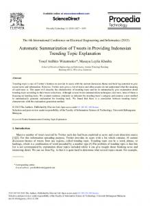
(15) Recalling that Wk is the intra-cluster NID, we substitute Wk (d ) , the randomly generated uniformly distributed data intra-cluster NID for the first term, and Wk (x ) , the intra-cluster NID for our data for the second term, G ( x ) Wk (d )  W k ( x ) . (16) Comparing eqns. (16) and (7) we see that the gap statistic and the randomness deficiency are identical except for the logarithms of the two terms. The logarithms in eqn. (7) can be interpreted as expressing a conventional distance measure (e.g. Euclidean) as a number of bits. When using the gap statistic with an NID based distance measure, the formulation in eqn. (16) should be used. 2.4 Quantization and the NCD For numeric time series, the performance of the NCD can be improved using quantization as a preprocessing step. Numeric time series data can be quantized to a given precision by histogramming the data [16]. Similar numeric values are assigned to the same histogram bin, and a representative value for that bin is used to represent all numeric values assigned to it. Placing the bins in the histogram such that each bin contains an equal number of data points maximizes the entropy of the quantization. In the SAX approach [17] and in [16] the data is assumed to have a normal distribution. Their implementation is limited by their use of a lookup table that defines the locations of a maximum of 10 bins, and one dimension. We propose a method that allows quantization of data of any dimension, to any number of symbols. If x [ x1 " x p ] is a p-dimensional normally distributed random variable with mean P and covariance 6 , then the equiprobable regions of x are ellipsoids [18]. First, define the quadratic form (17) Q ( x ) ( x  ȝ) T Ȉ 1 ( x  ȝ) , Q ( x ) is a chi-squared distributed random variable with p where degrees of freedom [18]. The hyper-ellipsoid Q ( x ) Ȥ 2 (1  D , p ) , (18) where Q(x) is given by eqn. (17), is the boundary of the 100D % confidence ellipse. The breakpoints, or boundary points separating symbols, are linearly spaced on the interval [0,1]. A symbol is assigned to x based on the region of the chi-squared inverse CDF that Q( x) falls into. 3. EXPERIMENTAL RESULTS A single implementation, as described in section 2, has been used to produce summaries of image sequence data from cell and tissue biology. Results are presented here for three diverse applications. Our method proceeds as follows. Starting with input image sequences (figure1, panel a), object extraction and tracking algorithms are run, generating time courses of object feature values (figure1, panel b). For each feature subset and number of quantization levels, a pairwise NAID matrix is generated (figure1, panel c). Feature subset selection can be done by exhaustively searching the feature space, or by using an implicit search method such as the floating search method [19]. The feature subset and number of quantization levels that maximize the gap statistic are chosen. The corresponding list of cluster assignments, along with the feature subset constitute our summary (figure1, panel d). In [9], Al Kofahi et al. presented a method for automatic

861

tracking and lineage tree construction from these image sequences. Neural progenitor cells differentiate into either glial cells or neurons in vitro. Currently, definitive classification of neurons versus glial and progenitor cells requires staining the culture for the molecule ȕ-tubulin III that selectively labels neurons. The staining process is fatal to cells in the culture, so can only be done after the image sequence recording is complete. Our summary automatically differentiated neurons from progenitor cells. The second application involves a dual-mode phase and fluorescence time-lapse image sequence showing a live neuron and a fluorescently labeled kinesin protein believed to play a role in axonal specification, the process whereby one of a developing cell’s neurites is chosen by the cell as the axon [20]. The data for this analysis was based on nine cell cultures. Since this image data contains more than one channel of information, and the fact that the associations between information in channels is of considerable scientific interest in its own right, we add features to the ATG that quantify associations. Specifically, at each time slice, we find the percentage of the kinesin protein closest to distal (growing) end of each neurite. This associative feature was then included in the same summarization analysis along with all other features. The resulting summary found two groups in the data, one consisting exclusively of neurons which had undergone axonal specification, the second consisting exclusively of neurons which had not undergone axonal specification. In [21], Chen et. al. describe a method for segmenting and tracking thymocytes. A heterogeneous population including P14 positive type and wild type thymocyte were imaged using a twophoton two-channel laser-scanning microscope. The ten datasets consisted of data on over 400 cells. Each dataset was treated as an object (e.g. each movie was one object), and included the time course of features from all t-cells from that dataset. Feature subset selection on the seven dimensional feature space identified cell volume as the feature which maximized the gap statistic. The resulting summary found two groups in the data. Each group corresponded exclusively to wild type or P14 type thymocyte cells. Figure 1 shows a sample image from each application, along with the ATG colored according to the summary results. 4. CONCLUSIONS AND DISCUSSION Our work demonstrates the practicality of using concepts from algorithmic information theory to summarize changes within and across image sequences in a manner that is theoretically optimal, and very powerful and straightforward in implementation. The generality of our methodology is an attractive feature for summarizing changes in individual image sequences, as well as changes across multiple image sequences. The three different application domains that we considered are actual problems of interest, but have in the past been treated with separate algorithm development efforts. Analyzing the lifespan and reproduction of neural progenitor cells generated a summary which separated neurons from glial and progenitor cells, a task which typically requires a toxic fixative stain. Analyzing the association between a cells’ neurites and a kinesin protein enabled the automatic identification of cells which had undergone axonal specification. Wild type and genetically modified thymocytes were automatically separated by the time course of cell volume. All of these applications were analyzed using a single implementation. Importantly, results that were meaningful in the informationtheoretic sense also proved to be biologically meaningful. Given the inherent generality of our approach, we are confident of broader applications.

ªd11 «d D « 21 «# « ¬dn1

(a)

(b)

d12 " d1n º d22 " d2n» » # # #» » dn2 " dnn¼

(c)

(e)

(d)

(f)

Figure 1. Sample images and ATG’s colored with summary results for the three application domains analyzed for this paper. Analyzing neural progenitor cells; (a) one image from input sequence, (b) object time course data, (c) NAID matrix obtained from pairwise comparison of object time course data, (d) summary resulting from gap spectral clustering of the NAID matrix showing neurons (red) differentiated from progenitor cells (blue), an accomplishment which until now has required the use of a toxic fixative stain. Analysis of thymocytes cells (e ) found volume to be a differentiating feature for wild type (blue) and generally modified (green) cells. The association of a kinesin proton with developing neurites (f) led to a summary which identified cells which had undergone axonal specification. Intelligence, IEEE Transactions on, 2000. 22(8): p. 747-757. 5. REFERENCES 12. Medioni, G., et al., Event detection and analysis from video streams. Pattern Analysis and Machine Intelligence, IEEE 1. Bennett, C.H., et al., Information distance. Information Transactions on, 2001. 23(8): p. 873 - 889. Theory, IEEE Transactions on, 1998. 44(4): p. 1407-1423. 13. Yianilos, P.N., Normalized Forms for Two Common Metrics 2. Cilibrasi, R. and P.M.B. Vitanyi, Clustering by compression. 1991, The NEC Research Institute, Technical Report: Information Theory, IEEE Transactions on, 2005. 51(4): p. Princeton, New Jersey. 1523-1545. 14. Ng, A.Y., M. Jordan, and Y. Weiss, On Spectral Clustering: 3. Li, M., et al., The similarity metric. Information Theory, IEEE Analysis and an algorithm. Advances in Neural Information Transactions on, 2004. 50(12): p. 3250-3264. Processing Systems 14, 2002. 4. Gacs, P., J. Tromp, and P. Vitanyi, Algorithmic statistics. IEEE 15. Tibshirani, R., G. Walther, and T. Hastie, Estimating the Trans. Inform. Theory, 2001. 47(6): p. 2443-2463. number of clusters in a dataset via the gap statistic. Journal of 5. Vereshchagin, N.K. and P.M.B. Vitanyi, Kolmogorov's the Royal Statistical Society, 2001. 63: p. 411 - 423. structure functions and model selection. Information Theory, 16. Chen, L. and M.T. Ozsu. Multi-scale histograms for answering IEEE Transactions on, 2004. 50(12): p. 3265-3290. queries over time series data. in Data Engineering, 2004. 6. Vitanyi, P., Meaningful information. IEEE Trans. Inform. Th., Proceedings. 20th International Conference on. 2004. 2006. 52(10): p. 4617 - 4626. 17. Lin, J., Keogh, E., Lonardi, S. & Chiu, B, A Symbolic 7. Cover, T.M. and J.A. Thomas, Elements of Information Representation of Time Series, with Implications for Streaming Theory. 1991: John Wiley. Algorithms. Data Mining and Knowledge Discovery Journal., 8. Al-Kofahi, O., et al., Automated semantic analysis of changes To appear. in image sequences of neurons in culture. Biomedical 18. Chew, V., Confidence, Prediction, and Tolerance Regions for Engineering, IEEE Transactions on, 2006. 53(6): p. 1109the Multivariate Normal Distribution. Journal of the American 1123. Statistical Association, 1966. 61(315): p. 605-617. 9. Al-Kofahi, O., et al., Automated cell lineage tracing: a high19. Pudil, P., et al., Floating search methods for feature selection throughput method to analyze cell proliferative behavior with nonmonotonic criterion functions. Pattern Recognition, developed using mouse neural stem cells. Cell Cycle, 2006. 1994. 2: p. 279-283 vol.2. 5(3): p. 327 - 335. 20. Jacobson, G., B. Schnapp, and G.A. Banker, A change in the 10. Narasimha-Iyer, H., et al., Integrated Analysis of Vascular and selective translocation of the Kinesin-1 motor domain marks Non-Vascular Changes from Color Retinal Fundus Image the initial specification of the axon. Neuron 2006. 49: p. 797Sequences. IEEE Transactions on Biomedical Engineering, 804. 2007. 54(8): p. 1436-45. 21. Chen, Y., et al., Automated 5-D Analysis of Cell Migration and 11. Stauffer, C. and W.E.L. Grimson, Learning patterns of activity Interaction in the Thymic Cortex from Time-Lapse Sequences using real-time tracking. Pattern Analysis and Machine of 3-D Multi-channel Multi-photon Images. In review, 2007.

862