Automatic Synthesis of both the Topology and ... - Semantic Scholar

Automatic Synthesis of both the Topology and Parameters for a Robust Controller for a Non-Minimal Phase Plant and a Three-Lag Plant by Means of Genetic Programming John R. Koza

Martin A. Keane

Jessen Yu

Section on Medical Informatics School of Medicine Stanford University Stanford, California 94305 [email protected] www.smi.stanford.edu/peo ple/koza

Econometrics Inc. 111 E. Wacker Dr. Chicago, Illinois 60601 [email protected]

Genetic Programming Inc. Box 1669 Los Altos, California 94023 [email protected]

Forrest H Bennett III

William Mydlowec

Oscar Stiffelman

Genetic Programming Inc. Box 1669 Los Altos, California 94023 [email protected] www.geneticprogramming.com

Genetic Programming Inc. Box 1669 Los Altos, California 94023 [email protected]

Computer Science Department Stanford University Stanford, California 94305 [email protected]

Abstract This paper describes how genetic programming can be used to automate the synthesis of the design of both the topology and parameter values for controllers. The method described in this paper automatically makes decisions concerning the total number of processing blocks to be employed in the controller, the type of each block, the topological interconnections between the blocks, the values of all parameters for the blocks, and the existence, if any, of internal feedback between the blocks of the overall controller. This design process can readily combine optimization of performance (e.g., by a metric such as the integral of the time-weighted error) with timedomain constraints and frequency-domain constraints. Genetic programming is applied to two illustrative problems of controller synthesis: the design of a robust controller for a non-minimal-phase plant and the design of a robust controller for a threelag plant. A previously published PID compensator (Astrom and Hagglund 1995) for the three-lag plant delivers credible performance. The automatically created controller is better than 7.2 times as effective as the previous controller as measured by the integral of the time-weighted absolute error, has only 50% of the rise time in response to the reference input, has only 35% of the settling time, and is 92.7 dB better in

terms of suppressing the effects of disturbance at the plant input.

1

Introduction

The process of creating (synthesizing) the design of a controller entails making decisions concerning the total number of processing blocks to be employed in the controller, the type of each block (e.g., lead, lag, gain, integrator, differentiator, adder, inverter, subtractor, and multiplier), the interconnections between the blocks, the values of all parameters for all the blocks, and the existence, if any, of internal feedback between the processing blocks. This process is typically channeled along lines established by existing mathematical techniques. For example, existing techniques often lead to a PID-type controller consisting of one proportional, one integrative, and one derivative processing block. It would be desirable to have an automatic system for creating the design of a controller that did not require the user to prespecify the topology of the controller (e.g. PID), but, instead, automatically produced both the overall topology and parameter values directly from a high-level statement of the requirements of the controller. This paper describes how genetic programming can be used to automatically create both the topology and parameter values for a controller. The automatically created controllers can accommodate

one or more externally supplied reference signals, external feedback of one or more plant outputs to the controller, computations of error between the reference signals and the corresponding external plant outputs, one or more internal state variables of the plant, and one or more control variables. These automatically created controllers can also accommodate internal feedback of one or more signals from one part of the controller to another part of the controller. In addition, this design process can readily combine optimization of performance (e.g., by a metric such as the integral of the time-weighted error) with time-domain constraints and frequencydomain constraints. Section 2 describes two illustrative control problems involving the design of a robust controller. Section 3 provides general background on genetic programming. Section 4 describes how genetic programming is applied to control problems. Section 5 describes the preparatory steps necessary to apply genetic programming to the two illustrative control problems. Sections 6 and 7 presents the results.

2

Two Illustrative Problems

The first illustrative problem is to create both the topology and parameter values for a robust controller for non-minimal-phase plant such that plant output reaches the level of the reference signal in minimal time, such that the overshoot in response to a step input is less than 2%, and such that the controller is robust in the face of significant variation in the plant's internal gain, K, and the plant's time constant, τ. Specifically, the transfer function of the nonminimal-phase plant is

K (1 − 0.5s) (1 + τs) 2 A controller is presented in Villagran and Sbarbaro (1998) and it delivers credible performance on this problem. The previously published controller is specialized for K = 1 and τ = 1 whereas the plant in this paper operates over several different combinations of values for K and τ. To make the problem more realistic, we added an additional constraint (satisfied by the controller of Villagran and Sbarbaro) limiting the input to the plant to the range between -40 and +40 volts. The second problem is to create both the topology and parameter values for a robust controller for a three-lag plant such that plant output reaches the level of the reference signal in minimal time, such that the overshoot in response to a step input is less than 2%, and such that the controller is robust in the face of significant variation in the plant's internal G ( s) =

gain, K, and the plant's time constant, τ. Specifically, the transfer function of the three-lag plant is

G(s) =

K

(1 + τs ) 3 The plant's internal gain, K, is varied from 1 to 2 and the plant's time constant, τ, is varied from 0.5 to 1.0. A PID controller is presented in Astrom and Hagglund (1995, page 225) and it delivers credible performance on this problem. To make the problem more realistic, we added the additional constraint (satisfied by the controller presented by Astrom and Hagglund) limiting the input to the plant to the range between -10 and +10 volts.

3

Background on Genetic Programming

Genetic programming is an automatic technique for generating computer programs to solve, or approximately solve, problems. In particular, genetic programming is capable of automatically creating the design of complex structures. Genetic programming (Koza 1992; Koza and Rice 1992) is an extension of the genetic algorithm (Holland 1975). Genetic programming is capable (Koza 1994a, 1994b) of evolving reusable, parametrized, hierarchically-called automatically defined functions (ADFs) so that an overall program consists of a main result-producing branch and one or more automatically defined functions (functiondefining branches). In addition, architecture-altering operations (Koza, Bennett, Andre, and Keane 1999; Koza, Bennett, Andre, Keane, and Brave 1999) enable genetic programming to automatically determine the number of automatically defined functions, the number of arguments that each possesses, and the nature of the hierarchical references, if any, among such automatically defined functions. Architecture-altering operations also enable genetic programming to automatically determine whether and how to use internal memory, iterations, and recursion. Genetic programming breeds computer programs to solve problems by executing the following three steps: (1) Randomly create an initial population of individual computer programs. (2) Iteratively perform the following substeps (called a generation) on the population of programs until the termination criterion has been satisfied: (a) Assign a fitness value to each program in the population using the fitness measure. (b) Create a new population of individual programs by applying the following three genetic

operations. The genetic operations are applied to one or two individuals in the population selected with a probability based on fitness (with reselection allowed). (i) Reproduction: Reproduce a selected individual by copying it into the new population. (ii) C r o s s o v e r : Create two new individual programs from two selected parental individuals by genetically recombining subtrees from each parental program using the crossover operation at randomly chosen crossover points in the parental programs. (iii) Mutation: Create a new individual from a selected parental individual by randomly mutating one randomly chosen subtree of the parental program. (iv) Architecture-altering operations: Choose an architecture-altering operation create one new offspring program for the new population by applying the architecturealtering operation to the selected program. (3) Designate the individual computer program that is identified by the method of result designation (e.g., the best-so-far individual) as the result of the run of genetic programming. This result may be a solution (or approximate solution) to the problem. Genetic programming often creates novel designs because it is a probabilistic process that is not encumbered by the preconceptions that often channel human thinking down familiar paths. G e n e t i c Programming: Darwinian Invention and Problem Solving (Koza, Bennett, Andre, and Keane 1999) and the accompanying videotape (Koza, Bennett, Andre, Keane, and Brave 1999) demonstrate that genetic programming is capable of synthesizing the design of both the topology and sizing for a wide variety of analog electrical circuits from a high-level statement of the circuit's desired behavior and characteristics. Five of the evolved analog circuits in that book infringe on previously issued patents while five others deliver the same functionality as previously patented inventions in a novel way. Additional information on current research in genetic programming can be found in Banzhaf, Nordin, Keller, and Francone 1998; Langdon 1998; Kinnear 1994; Angeline and Kinnear 1996; Spector, Langdon, O'Reilly, and Angeline 1999; Koza, Goldberg, Fogel, and Riolo 1996; Koza, Deb, Dorigo, Fogel, Garzon, Iba, and Riolo 1997; Koza, Banzhaf, Chellapilla, Deb, Dorigo, Fogel, Garzon, Goldberg, Iba, and Riolo 1998; Banzhaf, Poli, Schoenauer, and Fogarty 1998; Banzhaf, Daida, Eiben, Garzon, Honavar, Jakiela, and Smith 1999; Poli, Nordin, Langdon, and Fogarty 1999; in the new journal Genetic Programming and Evolvable

Machines (from Kluwer Academic Publishers) and at www.genetic-programming.org.

4 Genetic Programming and Control The output of a controller causes the actual response(s) of a process (called the plant) to match desired response(s), called the reference signal(s). In a closed loop controller, the difference(s) between the actual plant response(s) and the reference signal(s) are computed and fed back into the controller. Controllers are often represented by directed graphs in which the internal points represent certain functions, in which external points represent the controller's input(s), and in which cycles correspond to internal feedback within the controller. Genetic programming can be extended to the problem of creating both the topology and parameter values for a closed loop controller by establishing a mapping between the program trees used in genetic programming and the specialized type of directed graphs germane to controllers. Various functions and terminals may be included in the repertoire from which controllers can be constructed. The functions correspond to blocks in a block diagram representing a controller. The number of main result-producing branches in the to-be-evolved controller equals the number of control variables that are to be passed from the controller to the plant. Each result-producing branch is a composition of the functions and terminals from a repertoire (below) of functions and terminals. Programs trees in the population during the initial random generation (generation 0) consist only of result-producing branch(es). Automatically defined functions are introduced incrementally (and sparingly) into the population on subsequent generations by means of the architecture-altering operations. Each automatically defined function is a composition of the functions and terminals appropriate for control problems, references to existing automatically defined functions, and (possibly) dummy variables (formal parameters) that permit parameterization of the automatically defined function. In control problems, automatically defined functions provide a mechanism for internal feedback (recursion) within the to-be-evolved controller. Each branch of each program tree in the initial random population is created in accordance with a constrained syntactic structure. Each genetic operation (crossover, mutation, reproduction, and architecture-altering operation) produces offspring that comply with the constrained syntactic structure.

4.1

Repertoire of Functions

The functions may include the following: The two-argument GAIN function multiplies the time-domain signal represented by its first argument by a constant numerical factor represented by its second argument. The one-argument INVERTER function negates the time-domain signal represented by its argument. The DIFFERENTIAL_INPUT_INTEGRATOR function has two arguments and integrates the timedomain signal representing the difference between its two arguments. The two-argument LAG function applies the transfer function 1 / (1 + τs), where s is the Laplace operator and τ is a constant parameter. The first argument is the time-domain input signal. The second argument, τ, is numerically valued. The three-argument LAG2 function applies the transfer function

ω 02

, s 2 + 2ξω 0 s + ω 02 where s is the Laplace operator, ζ is the damping ratio, and ω0 is the corner frequency. The two-argument LEAD function applies the transfer function 1 + τs, where s is the Laplace operator and τ is a constant parameter. The first argument is the time-domain input signal. The second argument, τ, is numerically valued. The one-argument DIFFERENTIATOR function differentiates the time-domain signal represented by its argument. The two-argument A D D _ S I G N A L and S U B _ S I G N A L functions perform addition or subtraction, respectively, on the time-domain signals represented by their two arguments. The three-argument ADD_3_SIGNAL adds the time-domain signals represented by its three arguments.

4.2

Repertoire of Terminals

The terminals may include the following: The REFERENCE_SIGNAL is the time-domain signal representing the reference signal (desired plant response). The PLANT_OUTPUT is the plant output. The CONTROLLER_OUTPUT is the time-domain signal representing the output of the controller. Note that this signal can be used, if desired to provide feedback of the controller's output directly back into the controller. The CONSTANT_0_SIGNAL function is a timedomain signal that is always zero. Floating-point numerical constant terminals (ranging from -5.0 to +5.0) are represented by

arithmetic-performing subtrees (described in detail in Koza, Bennett, Andre, and Keane 1999) for the nonminimal phase problem and by perturbable numerical constants for the three-lag plant problem. They are interpreted on a logarithmic scale so that they represent values in a range of 10 orders of magnitude.

5

Preparatory Steps

Six major preparatory steps are required before applying genetic programming to a problem: (1) determine the architecture of the program trees, (2) identify the terminals, (3) identify the functions, (4) define the fitness measure, (5) choose control parameters for the run, and (6) choose the termination criterion and method of result designation.

5.1

Program Architecture

Since both problems involve one-output controllers, each program tree in the population has one resultproducing branch. Each program tree also has up to five automatically defined functions. Each program tree in the initial random population (generation 0) has no automatically defined functions. However, in subsequent generations, the architecture-altering operations may insert (and delete) automatically defined functions to particular individual program trees in the population.

5.2 Terminal Set The terminal set, T, is T = {CONSTANT_0, REFERENCE_SIGNAL, CONTROLLER_OUTPUT, PLANT_OUTPUT}.

5.3

Function Set

For the three lag plant problem, the function set, F, is F = {GAIN, INVERTER, LEAD, LAG, LAG2, DIFFERENTIAL_INPUT_INTEGRATOR, DIFFERENTIATOR, ADD_SIGNAL, SUB_SIGNAL, ADD_3_SIGNAL, ADF0, ADF1, ADF2, ADF3, ADF4}. Here ADF0, A D F 1, … denote the automatically defined functions added during the run by the architecture-altering operations. LAG2 is not used for the non-minimal phase plant problem.

5.4

Fitness

Genetic programming is a probabilistic search algorithm through the space of compositions of the available functions and terminals. The search is guided by a fitness measure. The fitness measure is a mathematical implementation of the high-level requirements of the problem. The fitness measure is couched in terms of “what needs to be done”  not “how to do it.”

The fitness measure may incorporate any measurable, observable, or calculable behavior or characteristic or combination of behaviors or characteristics. The fitness measure for most problems of controller design is multi-objective in the sense that there are several different (usually conflicting) requirements for the controller. Construction of the fitness measure requires translating the high-level requirements of the problem into a mathematically precise computation. The fitness of each individual is determined by executing the program tree (i.e., the result-producing branch and any automatically defined functions that may be present) to produce an interconnected sequence of signal processing blocks  that is, a block diagram for the controller. The netlist for the resulting controller is wrapped inside an appropriate set of SPICE commands and the controller is then simulated using our modified version of the SPICE simulator (Quarles, Newton, Pederson, and Sangiovanni-Vincentelli 1994). The SPICE simulator returns tabular and other information from which the fitness of the individual can be computed. Three-Lag Plant Problem For the three-lag plant problem, the fitness of a controller is measured using 10 elements, including (1) eight time-domain-based elements based on a modified integral of time-weighted absolute error (ITAE) measuring the rapidity of achievement of the desired value of the plant response, the controller's robustness, and the controller's minimization of overshoot, (2) one time-domain-based element measuring the controller's stability when faced with an extreme spiked reference signal, and (3) one time-domain-based element measuring disturbance rejection. The fitness of an individual controller is the sum of the detrimental contributions of these ten elements. The smaller the fitness, the better. The first eight elements of the fitness measure for the three-lag plant problem together evaluate how quickly the controller causes the plant to reach the reference signal, the robustness of the controller in face of significant variations in the plant's internal gain and the plant's time constant, and the success of the controller in avoiding overshoot. These eight elements of the fitness measure represent the eight choices of a particular one of two different values of the plant's internal gain, K, in conjunction with a particular one of two different values of the plant's time constant τ, in conjunction with a particular one of two different values for the height of the reference signal. The two values of K are 1.0 and 2.0. The two values of τ are 0.5 and 1.0. The first reference signal

is a step function that rises from 0 to 1 volts at t = 100 milliseconds. The second reference signal rises from 0 to 1 microvolts at t = 100 milliseconds. The two values of K and τ are used in order to obtain a robust controller. The two step functions are used to deal with the non-linearity caused by the limiter. For each of these eight fitness cases, a transient analysis is performed in the time domain using the SPICE simulator. The contribution to fitness for each of these eight elements of the fitness measure is based on the integral of time-weighted absolute error 9.6

∫ t e(t ) A(e(t )) Bdt .

t =0

Here e(t) is the difference (error) at time t between the plant output and the reference signal. We modified the integral of time-weighted absolute error in three ways. First, we used a discrete approximation to the integral by considering 120 80millisecond time steps between t = 0 to t = 9.6 seconds. Second, we multiplied each fitness case by the reciprocal of the amplitude of the reference signals so that both reference signals are equally influential. Specifically, B multiplies the difference e(t) associated with the 1-volt step function by 1 and multiplies the difference e(t) associated with the 1microvolt step function by 106. Third, the integral contains an additional weight, A , that varies depending on e (t). The function A weights all variations below the reference signal and all variations up to 2% above the reference signal by a factor of 1.0, but A heavily penalizes overshoots above 2% by a factor 10.0. The ninth element of the fitness measure for the three-lag plant problem evaluates the stability of the controller when faced with an extreme spiked reference signal. The spiked reference signal rises to 10-9 volts at time t = 0 and persists for 10nanoseconds. The reference signal is then 0 for all other times. An additional transient analysis is performed using the SPICE simulator for 121 fitness cases representing times t = 0 to t = 120 microseconds. If the plant output never exceeds a fixed limit of 10-8 volts (i.e., a order of magnitude greater than the pulse’s magnitude) for any of these 121 fitness cases, then this element of the fitness measure is zero. However, if the absolute value of plant output goes above 10-8 volts for any time t, then the contribution to fitness is 500(0.000120 - t), where t is first time (in seconds) at which the absolute value of plant output goes above 10-8 volts. This penalty is a ramp defined from the point (0, P) to (1.2, 0), where P = 0.06 seconds is the maximum penalty. The tenth element of the fitness measure for the three-lag plant problem is based on disturbance rejection. This tenth element is computed based on a

time-domain analysis for 9.6 seconds. In this analysis, the reference signal is held at a value of 0. A disturbance signal consisting of a unit step is added to the CONTROLLER_OUTPUT at time t = 0 and the resulting disturbed signal is provided as input to the plant. The detrimental contribution to fitness is the absolute value of the largest single difference between the plant output and the reference signal (which is invariant at 0 throughout). A controller that cannot be simulated by SPICE is assigned a high penalty value of fitness (108). Non-Minimal Phase Plant Problem This problem illustrates that a frequency domain constraint can be readily intermixed with optimization requirements and time-domain constraints in the fitness measure. The fitness measure for the non-minimal phase plant problem consists of 11 elements. The first nine elements are identical to that above. The tenth element is identical, except that the test is performed for 2.4 seconds. The eleventh element of the fitness measure for the non-minimal phase plant problem reflects a desire to avoid responding to highfrequency perturbations in the reference signal. This eleventh element is based on 121 fitness cases representing an AC sweep of the reference signal over 20 sampled frequencies (equally spaced on a logarithmic scale) in each of six decades of frequency between 0.01 Hz and 10,000 Hz. A gain of 0 dB is ideal for the 80 fitness cases in the first four decades of frequency between 0.01 Hz and 100 Hz; however, a gain of up to +3 dB is acceptable. The detrimental contribution to fitness for each of these 80 fitness cases is zero if the gain is ideal or acceptable, but 18/121 per fitness case otherwise. The ideal gain for the 41 fitness cases in the two decades between 100 Hz and 10,000 Hz is given by the straight line connecting (100 Hz, -3 dB) and (10,000 Hz, -83 dB) with a logarithmic horizontal axis and a linear vertical axis. The detrimental contribution to fitness for each of these fitness cases is zero if the gain is on or below this straight line, but 18/121 per fitness case otherwise.

5.5

Control Parameters

The population size, M, was 66,000. A maximum size of 150 points (for functions and terminals) was established for each result-producing branch and a maximum size of 100 points was established for each automatically defined function. The other parameters for controlling the runs are the default values that we apply to a broad range of problems (Koza, Bennett, Andre, and Keane 1999).

5.6

Termination

The run was manually monitored and manually terminated when the fitness of many successive bestof-generation individuals appeared to have reached a plateau. The single best-so-far individual is harvested and designated as the result of the run.

5.7

Parallel Implementation

This problem was run on a home-built Beowulf-style (Sterling, Salmon, Becker, and Savarese 1999; Bennett, Koza, Shipman, and Stiffelman 1999) parallel cluster computer system consisting of 66 processing nodes (each containing a 533-MHz DEC Alpha microprocessor and 64 megabytes of RAM). The processing nodes are connected with a 100 megabit-per-second Ethernet. The processing nodes and the DEC Alpha type host use the Linux operating system. The distributed genetic algorithm (Andre and Koza 1996) was used with a population size of Q = 1,000 at each of the D = 66 demes (semi-isolated subpopulations). Generations are asynchronous on the nodes. On each generation, four boatloads of emigrants, each consisting of B = 2% of the node's subpopulation (each selected probabilistically on the basis of fitness) emigrate to adjacent processing nodes. For additional information, visit www.genetic-programming.com.

6

Results for Non-Minimal Phase Plant

The best individual from the initial random generation (generation 0) for the non-minimal phase plant problem has a fitness of 94.99. The best-of-run individual from generation 38 has a fitness of 21.72. Table1 shows the contribution of each of the 11 elements of the fitness measure. Table 1 Fitness of best-of-run individual for nonminimal phase plant problem Step size

Internal Gain, K 1 1 1 2 1 1 3 1 2 4 1 2 5 10-6 1 6 10-6 1 7 10-6 2 8 10-6 2 9 Spiked reference signal 10 Disturbance rejection 11 AC sweep TOTAL

Time constant 1.0 0.5 1.0 0.5 1.0 0.5 1.0 0.5

Fitness 3.00 3.94 1.54 2.12 3.00 3.94 1.54 2.14 0.00 0.49 0.00 21.72

Figure 1 shows the evolved best-of-run individual from generation 38 (at the left of the figure) and the non-minimal phase plant (on the right). Figure 2 compares the plant response in the time domain for the best-of-run individual (dashed curve) and the controller presented by Villagran and Sbarbaro (solid curve). The transfer functions for the best-of-run individual from generation 38 are

H ( s) =

(

1.13 1.67 + 1.78s + s 2 s(2.51 + s )

(

) )

0.221(6.13 + s )1.23 + 2.16 s + s 2 1.67 + 1.78s + s 2 The evolved controller performs robustly. A Bode plot for the entire system (not shown) confirms that the evolved controller conforms to the desired 40db/decade roll-off at frequencies higher than 100Hz. F (s) =

7

(

)

Results for Three-Lag Plant

The best individual from generation 0 of our one and only run of this problem has a fitness of 14.35. The best-of-run individual emerged in generation 31 and had a near-zero fitness of 1.14. Figure 3 shows this individual controller in the form of a block diagram. Table 2 shows (for each of the eight combinations of step size, internal gain, K, and time constant, τ) the values of disturbance rejection (in microvolts out per disturbance volt), integral of time-weighted error (in volt-second2), closed loop bandwidth (in Hertz), rise time (90%), and settling time (2%), for the best-ofrun individual of generation 31 for three-lag plant. The system bandwidth is the frequency of the reference signal above which the plant’s output is attenuated by at least a specified degree (3db here) in comparison to the plant’s output at a specified lower frequency (e.g., DC or very low frequencies). Table 3 shows (for each of the eight combinations of step size, internal gain, K, and time constant, τ) the values of disturbance rejection (in microvolts out per disturbance volt), integral of time-weighted error (in volt-second2), closed loop bandwidth (in Hertz), rise time (90%), and settling time (2%), for the PID solution (Astrom and Hagglund 1995) for three-lag plant. Astrom and Hagglund (1995) did not consider seven of the eight combinations of values for K, τ, and the step size used in computing the averages in table 6, whereas we used all eight combinations of values in our run. Accordingly, table 3 compares the performance of the best-of-run controller from generation 31 for the three-lag plant and the PID controller (Astrom and Hagglund 1995) for the

specific value of plant internal gain, K, of 1.0 used in Astrom and Hagglund, the specific value of the plant time constant τ, of 1.0 used in Astrom and Hagglund, and the specific step size of the reference signal (1.0 volts) used in Astrom and Hagglund. As can be seen in table 4, the best-of-run genetically evolved controller from generation 31 is 7.2 times better than the textbook controller as measured by the integral of the time-weighted absolute error, has only 50% of the rise time in response to the reference input, has only 35% of the settling time, and is 92.7 dB better in terms of suppressing the effects of disturbance at the plant input. The genetically evolved controller has 2.9 times the bandwidth of the PID controller.

References Andre, David and Koza, John R. 1996. Parallel genetic programming: A scalable implementation using the transputer architecture. In Angeline, P. J. and Kinnear, K. E. Jr. (editors). 1996. Advances in Genetic Programming 2. Cambridge: MIT Press. Angeline, Peter J. and Kinnear, Kenneth E. Jr. (editors). 1996. Advances in Genetic Programming 2. Cambridge, MA: The MIT Press. Astrom, Karl J. and Hagglund, Tore. 1995. P I D Controllers: Theory, Design, and Tuning. Second Edition. Research Triangle Park, NC: Instrument Society of America. Banzhaf, Wolfgang, Daida, Jason, Eiben, A. E., Garzon, Max H., Honavar, Vasant, Jakiela, Mark, and Smith, Robert E. (editors). 1999. GECCO-99: Proceedings of the Genetic and Evolutionary Computation Conference, July 13-17, 1999, Orlando, Florida USA. San Francisco, CA: Morgan Kaufmann. Banzhaf, Wolfgang, Nordin, Peter, Keller, Robert E., and Francone, Frank D. 1998. G e n e t i c Programming – An Introduction. San Francisco, CA: Morgan Kaufmann and Heidelberg: dpunkt. Banzhaf, Wolfgang, Poli, Riccardo, Schoenauer, Marc, and Fogarty, Terence C. 1998. Genetic Programming: First European Workshop. EuroGP'98. Paris, France, April 1998 Proceedings. Paris, France. April l998. Lecture Notes in Computer Science. Volume 1391. Berlin, Germany: Springer-Verlag. Bennett, Forrest H III, Koza, John R., Shipman, James, and Stiffelman, Oscar. 1999. Building a parallel computer system for $18,000 that performs a half peta-flop per day. In Banzhaf, Wolfgang, Daida, Jason, Eiben, A. E., Garzon, Max H.,

Honavar, Vasant, Jakiela, Mark, and Smith, Robert E. (editors). 1999. GECCO-99: Proceedings of the Genetic and Evolutionary Computation Conference, July 13-17, 1999, Orlando, Florida USA. San Francisco, CA: Morgan Kaufmann. Holland, John H. 1975. Adaptation in Natural and Artificial Systems. Ann Arbor, MI: University of Michigan Press. Kinnear, Kenneth E. Jr. (editor). 1994. Advances in Genetic Programming. Cambridge, MA: The MIT Press. Koza, John R. 1992. Genetic Programming: On the Programming of Computers by Means of Natural Selection. Cambridge, MA: MIT Press. Koza, John R. 1994a. Genetic Programming II: Automatic Discovery of Reusable Programs. Cambridge, MA: MIT Press. Koza, John R. 1994b. Genetic Programming II Videotape: The Next Generation. Cambridge, MA: MIT Press. Koza, John R., Banzhaf, Wolfgang, Chellapilla, Kumar, Deb, Kalyanmoy, Dorigo, Marco, Fogel, David B., Garzon, Max H., Goldberg, David E., Iba, Hitoshi, and Riolo, Rick. (editors). 1998. Genetic Programming 1998: Proceedings of the Third Annual Conference. San Francisco, CA: Morgan Kaufmann. Koza, John R., Bennett III, Forrest H, Andre, David, and Keane, Martin A. 1999. Genetic Programming III: Darwinian Invention and Problem Solving. San Francisco, CA: Morgan Kaufmann. Forthcoming. Koza, John R., Bennett III, Forrest H, Andre, David, Keane, Martin A., and Brave Scott. 1999. Genetic Programming III Videotape. San Francisco, CA: Morgan Kaufmann. Forthcoming. Koza, John R., Deb, Kalyanmoy, Dorigo, Marco, Fogel, David B., Garzon, Max, Iba, Hitoshi, and Riolo, Rick L. (editors). 1997. Genetic Programming 1997: Proceedings of the Second Annual Conference San Francisco, CA: Morgan Kaufmann. Koza, John R., Goldberg, David E., Fogel, David B., and Riolo, Rick L. (editors). 1996. G e n e t i c Programming 1996: Proceedings of the First Annual Conference. Cambridge, MA: MIT Press. Koza, John R., and Rice, James P. 1992. Genetic Programming: The Movie. Cambridge, MA: MIT Press.

Langdon, William B. 1998. Genetic Programming and Data Structures: Genetic Programming + Data Structures = Automatic Programming! Amsterdam: Kluwer. Poli, Riccardo, Nordin, Peter, Langdon, William B., and Fogarty, Terence C. 1999. G e n e t i c Programming: Second European Workshop. EuroGP'99. Proceedings. Lecture Notes in Computer Science. Volume 1598. Berlin: SpringerVerlag. Quarles, Thomas, Newton, A. R., Pederson, D. O., and Sangiovanni-Vincentelli, A. 1994. SPICE 3 Version 3F5 User's Manual. Department of Electrical Engineering and Computer Science, Univ. of California. Berkeley, CA. March 1994. Spector, Lee, Langdon, William B., O'Reilly, UnaMay, and Angeline, Peter (editors). 1999. Advances in Genetic Programming 3. Cambridge, MA: MIT Press. Sterling, Thomas L., Salmon, John, Becker, D. J., and Savarese, D. F. 1999. How to Build a Beowulf: A Guide to Implementation and Application of PC Clusters. Cambridge, MA: MIT Press. Villagran, Victor and Sbarbaro, Daniel. 1998. A new approach for turning PID controller based on iterative learning. Proceedings of the 1998 IEEE International Conference on Control Applications. Volume I. Pages 139 - 143.

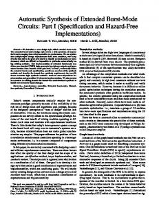
Figure 2 Comparison of evolved best-of-run individual from generation 38 (dashed curve) and previous result for non-minimal-phase plant (solid curve).

Figure 1 Best-of-run genetically evolved controller from generation 38 controller and plant for non-minimalphase plant problem.

Figure 3 Best-of-run genetically evolved controller from generation 31 for the three-lag plant. Table 2 Characteristics of best-of-run individual of generation 31 for the three-lag plant. τ Step size K Disturban ITAE Bandwidt Rise time ce h 1 1 1 1.0 4.3 0.360 0.72 1.25 2 1 1 0.5 4.3 0.190 0.72 0.97 3 1 2 1.0 4.3 0.240 0.72 0.98 4 1 2 0.5 4.3 0.160 0.72 0.90 5 10-6 1 1.0 4.3 0.069 0.72 0.64 6 10-6 1 0.5 4.3 0.046 0.72 0.53 7 10-6 2 1.0 4.3 0.024 0.72 0.34 8 10-6 2 0.5 4.3 0.046 0.72 0.52 AVERA 4.3 0.142 0.72 0.77 GE Table 3 Characteristics of PID solution (Astrom and Hagglund 1995) for the three-lag plant. τ Step size K Disturban ITAE Bandwidt Rise time ce h 1 1 1 1.0 186,000 2.6 0.248 2.49 2 1 1 0.5 156,000 2.3 0.112 3.46 3 1 2 1.0 217,000 2.0 0.341 2.06 4 1 2 0.5 164,000 1.9 0.123 3.17 5 10-6 1 1.0 186,000 2.6 0.248 2.49 6 10-6 1 0.5 156,000 2.3 0.112 3.46 7 10-6 2 1.0 217,000 2.0 0.341 2.06 8 10-6 2 0.5 164,000 1.9 0.123 3.17

Settling time 1.87 1.50 1.39 1.44 1.15 0.97 0.52 0.98 1.23

Settling time 6.46 5.36 5.64 4.53 6.46 5.36 5.64 4.53

AVERA GE

180,750

2.2

0.21

2.8

5.5

Table 4 Comparison of characteristics for K = 1.0, τ = 1.0, and step size of 1.0 for the three-lag plant. Units Genetically evolved Astrom and Hagglund controller 1995 controller Disturbance sensitivity µvolts /volt 4.3 186,000 ITAE volt sec2 0.360 2.6 Bandwidth (3dB) Hz 0.72 0.248 Rise time seconds 1.25 2.49 Settling time seconds 1.87 6.46