AUTOMATIC SYNTHESIS USING GENETIC PROGRAMMING OF ...

AUTOMATIC SYNTHESIS USING GENETIC PROGRAMMING OF IMPROVED PID TUNING RULES

Matthew J. Streeter1, Martin A. Keane2, and John R. Koza3 1

Genetic Programming, Inc. 2Econometrics, Inc. 3Stanford University

Abstract: Astrom and Hagglund developed tuning rules in 1995 for PID controllers that outperform the 1942 Ziegler-Nichols rules on an industrially representative set of plants. In this paper, we use genetic programming to automatically discover tuning rules for PID controllers that outperform the Astrom-Hagglund rules for the industrially representative set of plants specified by Astrom and Hagglund. Copyright © 2002 IFAC Keywords: Genetic programming, PID control 1

INTRODUCTION

The PID controller was patented in 1939 by Albert Callender and Allan Stevenson of Imperial Chemical Limited (Callender and Stevenson 1939). The 1942 Ziegler-Nichols tuning rules provided a relatively simple and effective method for determining the parameter values for the proportional, integrative, and derivative blocks of the PID controller (Ziegler and Nichols 1942). The Ziegler-Nichols tuning rules remain in widespread use today for tuning PID controllers. In their 1995 book PID Controllers: Theory, Design, and Tuning, Astrom and Hagglund identified four families of plants "that are representative for the dynamics of typical industrial processes." The first of the four families of plants in Astrom and Hagglund 1995 consists of plants represented by transfer functions of the form e -s (1 + sT ) 2 where T = 0.1, … , 10. G ( s) =

(A)

The second family consists of the n-lag plants represented by transfer functions of the form 1 (B) G ( s) = (1 + s ) n where n = 3, 4, and 8. The third family consists of plants represented by transfer functions of the form 1 (C) G ( s) = (1 + s )(1 + αs )(1 + α 2 s )(1 + α 3 s ) where α = 0.2, 0.5, and 0.7.

The fourth family consists of plants represented by transfer functions of the form 1 - αs (D) G ( s) = (s+1 )3 where α = 0.1, 0.2, 0.5, 1.0, and 2.0. Astrom and Hagglund developed a method in their 1995 book for automatically tuning PID controllers for all the plants in all four of these industrially representative families of plants. In one version of their method, Astrom and Hagglund use two frequency-domain parameters, namely the ultimate gain, Ku, and the ultimate period, Tu. Astrom and Hagglund describe a procedure for estimating these parameters from the plant's response to a step input. The tuning rules developed by Astrom and Hagglund in their 1995 book outperform the widely used Ziegler-Nichols tuning rules on all 16 industrially representative plants used by Astrom and Hagglund. As Astrom- Hagglund observe, “[Our] new methods give substantial improvements in control performance while retaining much of the simplicity of the Ziegler-Nichols rules.” The PID tuning rules devised by Astrom and Hagglund in 1995 are given by four equations. Reference Signal

204

200 Plant Feedback 206

210

Equation 1

+

230

220

Equation 2 -

202

+ 240 208

-

250

260

Equation 3

1/s

+

+ +

270

280

290

-1

Equation 4

s

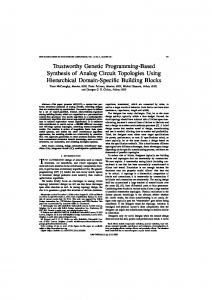
Fig. 1. PID controller

232

Control Variable

234

Referring to figure 1 (which shows a PID controller), equation 1 implements setpoint weighting, b, for the input to the proportional block 230 and is 0.56 -0.12 + Ku K 2 u 0.25* e

b= Equation 2 (for gain block 230) is the gain, Kp, that is associated with proportional block and is

Kp = 0.72 * Ku

-1.6 1.2 + Ku K 2 u *e

Equation 3 (for gain block 250) is the gain, Ki, that is associated with integrative block and is

Ki =

0.72* Ku

-1.6 1.2 + Ku K 2 u *e

0.59* Tu

-1.3 0.38 + Ku K 2 u *e

Equation 4 (for gain block 280) is the gain, Kd, that is associated with derivative block and is

Kd = 0.108* Ku * Tu

-1.6 1.2 + Ku K 2 u *e

-1.4 0.56 + Ku K 2 u *e

The transfer function for the Astrom-Hagglund PID controller is given by the equation: K A = K p (b * R - P ) + i ( R - P ) + K d * s * ( - P ) s where A is the output of the Astrom-Hagglund controller, R is the reference signal, P is the plant output, and b, Kp, Ki, and Kd are given above. The tuning rules developed by Astrom and Hagglund in their 1995 book outperform the widely used Ziegler-Nichols tuning rules (Ziegler and Nichols 1942) on all 16 industrially representative plants used by Astrom and Hagglund. The question arises as to whether there are tuning rules that may improve on the Astrom-Hagglund rules. Boyd and Barratt state in Linear Controller Design: Limits of Performance (Boyd and Barratt 1991), "The challenge for controller design is to productively use the enormous computing power available. Many current methods of computer-aided controller design simply automate procedures developed in the 1930's through the 1950's, for example, plotting root loci or Bode plots. Even the 'modern' state-space and frequency-domain methods (which require the solution of algebraic Riccati equations) greatly underutilize available computing power." In this paper, we use genetic programming to automatically discover PID tuning rules that outperform the automatic tuning rules developed by Astrom and Hagglund in 1995 for the industrially representative set of plants used by Astrom and Hagglund.

Section 2 provides background on genetic programming. Section 3 describes the preparatory steps required to apply genetic programming to the problem of automatically discovering tuning rules for PID controllers. Section 4 presents the results. 2

GENETIC PROGRAMMING

Genetic programming (Koza, Bennett, Andre, and Keane 1999; Koza, Keane, Streeter, Mydlowec, Yu, and Lanza 2003) is an automated method for solving problems. Specifically, genetic programming progressively breeds a population of computer programs over a series of generations. Genetic programming starts with a primordial ooze of thousands of randomly created computer programs and uses the Darwinian principle of natural selection, recombination (crossover), mutation, gene duplication, gene deletion, and certain mechanisms of developmental biology to breed an improved population over a series of many generations. Genetic programming breeds computer programs to solve problems by executing the following three steps: (1) Generate an initial population of compositions (typically random) of the functions and terminals of the problem. (2) Iteratively perform the following substeps (referred to herein as a generation) on the population of programs until the termination criterion has been satisfied: (A) Execute each program in the population and assign it a fitness value using the fitness measure. (B) Create a new population of programs by applying the following operations. The operations are applied to program(s) selected from the population with a probability based on fitness (with reselection allowed). (i) Reproduction: Copy the selected program to the new population. (ii) Crossover: Create a new offspring program for the new population by recombining randomly chosen parts of two selected programs. (iii) Mutation: Create one new offspring program for the new population by randomly mutating a randomly chosen part of the selected program. (iv) Architecture-altering operations: Select an architecture-altering operation from the available repertoire of such operations and create one new offspring program for the new population by applying the selected architecture-altering operation to the selected program. (3) Designate the individual program that is identified by result designation (e.g., the best-sofar individual) as the result of the run of genetic programming. This result may be a solution (or an approximate solution) to the problem.

3

PREPARATORY STEPS

Before applying genetic programming to a problem involving the synthesis of a controller, the human user of genetic programming must perform six major preparatory steps: (1) determine the architecture of the program trees, (2) identify the terminals, (3) identify the functions, (4) define the fitness measure, (5) choose control parameters for the run, and (6) specify the termination criterion for the run. Initial experimentation quickly confirmed to us that the Astrom and Hagglund tuning rules are highly effective. Starting from scratch, genetic programming was readily able to evolve four multidimensional surfaces that were very similar to the Astrom and Hagglund surfaces and that outperformed the Astrom and Hagglund tuning rules on average. However, the genetically evolved surfaces did not outperform the Astrom and Hagglund tuning rules across the board for every plant. Thus, we decided to approach the problem of discovering improved tuning rules by building on the Astrom and Hagglund results. Specifically, we used genetic programming to evolve four mathematical expressions which, when added to the four mathematical expressions devised by Astrom and Hagglund, yield improved overall performance. Note that any surface can emerge from this additive approach. 3.1 Program Architecture We are seeking four mathematical expressions for four quantities (Kp, Ki, Kd, and b). The four mathematical expressions contain free variables representing the plant’s ultimate gain, Ku, and the plant’s ultimate period, Tu. Thus, the architecture of each program tree in the population has four resultproducing branches (one each for Kp, Ki, Kd, and b). Note that this problem can be viewed as a problem of discovering four multi-dimensional surfaces. 3.2 Terminal Set The terminal set, T, or each of the four resultproducing branches contains T = {ℜ, KU, TU}. where KU represents the plant’s ultimate gain, Ku, and TU represents the plant’s ultimate period, Tu. Here ℜ denotes a perturbable numerical value. In the initial random generation (generation 0) of a run, each perturbable numerical value is set, individually and separately, to a random value in a chosen range (between –5.0 and +5.0 for this problem). 3.3 Function Set The function set, F, for each of the four resultproducing branches contains functions for performing arithmetic, exponential, and logarithmic operations. F = {ADD_NUMERIC, SUB_NUMERIC, MUL_NUMERIC, DIV_NUMERIC, REXP, RLOG, POW}.

The first six functions perform addition, subtraction, multiplication, division, exponential, and logarithm operations, respectively. The two-argument POW function returns the value of its first argument to the power of the value of its second argument. All functions are protected in the sense that they cannot yield a result whose absolute value is larger than 1015. These functions (along with the terminals from the previous section) are the ingredients for the four tuning rule equations that are to be produced by genetic programming. 3.4 Fitness Measure Genetic programming is a probabilistic algorithm that searches the space of compositions of the available functions and terminals under the guidance of a fitness measure. The fitness measure is a mathematical implementation of the problem's highlevel requirements. In this paper, genetic programming is being used to automatically create four equations using a fitness measure built from the same elements used in Astrom and Hagglund 1995. That is, our fitness measure attempts to optimize for the integral of the time-weighted absolute error (ITAE) for a step input and also to optimize for maximum sensitivity and sensor noise attenuation. We use the SPICE simulator (Quarles, Pederson, Newton, Sangiovanni-Vincentelli 1994) to simulate controllers. A SPICE netlist is constructed to represent the signal processing functions (gain, differentiator, integrator, addition, subtracting) of a PID controller with setpoint weighting, the plant, and the external feedback loop. This SPICE netlist is wrapped inside an appropriate set of commands to carry out various analyses in the time domain and in the frequency domain. We also provide SPICE with subcircuit definitions to implement all the signal processing functions necessary to represent the plant and the PID controller with setpoint weighting. The entire control system is then simulated using our modified version of the original 217,000-line SPICE3 simulator as a submodule within our genetic programming system. The genetic programming code then uses SPICE’s output to calculate the fitness of an individual controller. We use a test bed consisting of 30 different plants for this problem. Each of the 30 plants is from one of the four families (A, B, C, and D) of plants considered by Astrom and Hagglund in their 1995 book. We use more than the 16 plants used by Astrom and Hagglund to reduce the likelihood of over-fitting (particularly for the families for which Astrom and Hagglund consider only three plants). The 30 plants are identified in columns 1 and 2 of table 2. We subsequently use an additional 18 plants (again from the same four families) to cross-validate the results. The 18 additional plants are identified in columns 1 and 2 of table 3.

The fitness of each controller in the population is measured by means of eight separate invocations of the SPICE simulator for each plant. Since there are a total of 30 plants, the fitness measure entails 240 separate invocations of the SPICE simulator. This multi-part fitness measure attempts to optimize step response and disturbance rejection while simultaneously imposing constraints on maximum sensitivity and sensor noise attenuation. The fitness of an individual controller is the sum, over the eight fitness cases for each of the 30 plants under consideration, of the detrimental contributions to fitness. The smaller the sum, the better. Step response and disturbance rejection is measured by means of the first six of the eight SPICE simulations for each plant under consideration. For each plant under consideration, six combinations of values (shown in table TTTTWOFAMILIES1) for the height of the reference signal and disturbance signal are considered. The reference signal is a step function that rises from 0 at time t = 0 to a specified height at t = 1 millisecond. The reference signal is one of the inputs to the controller. The disturbance signal is a step function that rises from 0 at time t = 10Tu to a specified height at t = 10Tu + 1 millisecond. The disturbance signal is added to the controller's output. Table 1. Six combinations of height of reference and disturbance signals. Reference signal 1.0 10-3 -10-6 1.0 -1.0 0.0

Disturbance signal 1.0 10-3 10-6 -0.6 0.0 1.0

For each of the 30 plants under consideration, a transient analysis is performed in the time domain using the SPICE simulator for each of the six combinations of height of reference and disturbance signals in table 1. The function e(t) is the difference (error) at time t between the plant output and the reference signal. The contribution to fitness for each of these 180 elements is based on the sum of two integrals of time-weighted absolute error. The first term of the integral accounts for the controller's step response while the second term accounts for disturbance rejection. 20Tu

10Tu

∫ t e(t ) Bdt

t =0

Tu2

∫ (t − 10Tu ) e(t ) Cdt

+

t =10Tu

Tu2

.

The factor B in the first term of the integral multiplies each value of e(t) by the reciprocal of the amplitude of the reference signal (so that all reference signals are equally influential). The factor C in the second term of the integral multiplies the value of e(t) by the reciprocal of the amplitude of the disturbance signals. When the amplitude of either the reference signal or the disturbance signal is zero, the appropriate factor (B or C) is set to zero. The ITAE

component of fitness is such that, all other things being equal, changing the time scale by a factor of F changes the ITAE by F2. The division of the integral by Tu2 is an attempt to eliminate this artifact of the time scale and equalize the influence of each of the plants in the overall fitness measure. For these six elements of the fitness measure for each plant, the contribution to fitness is multiplied by 20 if the element is greater than that for the Astrom and Hagglund controller (1995). Stability margin is measured by means of the seventh SPICE simulation for each plant under consideration. Figure 2 presents a model for the entire system containing the given plant and the to-be-evolved controller. In this figure, R(s) is the reference signal; Y(s) is the plant output; and U(s) is the controller's output. Disturbance D(s) may be added to the controller's output U(s). Sensor noise N(s) may be added to the plant's output Y(s) yielding Q(s). Here N(s) is an AC signal. For each plant under consideration, an AC sweep is performed using the SPICE simulator from 1/(1000Tu) to 1000/Tu while holding the reference signal R(s) and the disturbance signal D(s) at zero. The maximum sensitivity, Ms, is a measure of the stability margin. It is desirable to minimize the maximum sensitivity (and therefore maximize the stability margin). The quantity 1/Ms is the minimum distance between the Nyquist plot and the point (-1,0) and is the stability margin incorporating both gain and phase margin. The maximum sensitivity is the maximum amplitude of Q(s). The contribution to fitness is 0 if Ms < 1.5; 2(Ms - 1.5) for 1.5 ≤ Ms ≤ 2.0; and 20(Ms - 2.0) + 1 for Ms > 2.0. For each plant under consideration, the contribution to fitness is multiplied by 10 if the element is greater than that for the Astrom and Hagglund controller (1995). D(s) R(s)

+

U(s) Controller

Y(s) Plant

+

Q(s)

+

+ N(s)

Fig. 2. Overall model Sensor noise attenuation is measured by means of the eighth SPICE simulation for each plant under consideration. Achieving favorable sensor noise attenuation is often in direct conflict with the goal of achieving a rapid response to setpoint changes and rejection of plant disturbances. For each plant under consideration, an AC sweep is performed using the SPICE simulator from 10/Tu to 1000/Tu while holding the reference signal R(s) and the disturbance signal; D(s) at zero. The attenuation of sensor noise is measured at plant output at Y(s). Amin is the minimum attenuation in decibels within this frequency range. It is desirable to maximize the minimum attenuation. The contribution to fitness for

sensor noise attenuation is 0 if Amin > 40 dB; (40 Amin)/10 if 20 dB ≤ Amin ≤ 40 dB; and 2 + (20 - Amin) if Amin < 20 dB. For each plant under consideration, the contribution to fitness is multiplied by 10 if the element is greater than that for the Astrom and Hagglund controller (1995). A controller that cannot be simulated by SPICE is 8 assigned a high penalty value of fitness (10 ). 3.5 Control Parameters The population size, M, is 100,000. The remaining control parameters are in Koza, Keane, Streeter, Mydlowec, Yu, and Lanza 2003. 3.6 Termination Criterion We manually monitored and terminated the run when fitness appeared to reach a plateau. 4

RESULTS

In the one run we made on this problem, PID tuning rules emerged on generation 76 that outperform the PID tuning rules in Astrom and Hagglund 1995. The improved tuning rules are obtained by adding the genetically evolved quantities below to the values of Kp, Ki, and Kd, and b in Astrom and Hagglund 1995. The quantity, Kp-adj, that is to be added to Kp for the proportional part of the controller is -.0012340 * Tu - 6.1173*10-6 The quantity, Ki-adj, that is to be added to Ki for the integrative part of the controller is Ku -.068525* Tu The quantity, Kd-adj, that is to be added to Kd for the derivative part of the controller is

( )log(1.6342

log Ku

)

-0.0026640 eTu The quantity, badj, that is to be added to b for setpoint weighting of the proportional block is Ku e Ku The authors refer to these evolved tuning rules as the Keane-Koza-Streeter (KKS) PID tuning rules.

Table 2 compares the performance of the best-of-run genetically evolved PID tuning rules from generation 76 as a percentage of the value for the Astrom and Hagglund controller for the 30 plants used by the evolutionary process. An “OK” appears in the table for the case where both controllers have a value of 0. As can be seen in the table, all percentages are either below 100% (indicating improvement) or “OK.” Table 3 compares the performance of the best-of-run genetically evolved PID tuning rules from generation 76 as a percentage of the value for the Astrom and Hagglund controller for the additional 18 plants used to cross-validate the results produced by the evolutionary process. As can be seen in the table, all

percentages are either below 100% (indicating improvement) or “OK.” Averaged over the 30 plants used by the evolutionary process, the best-of-run tuning rules from generation 76 have • 91.6% of the setpoint ITAE of the AstromHagglund tuning rules, • 96.2% of the disturbance rejection ITAE of the Astrom-Hagglund tuning rules, • 99.5% of the reciprocal of minimum attenuation of the Astrom-Hagglund tuning rules, and • 98.6% of the maximum sensitivity, Ms, of the Astrom-Hagglund tuning rules. Averaged over the 18 additional plants, the best-ofrun tuning rules from generation 76 have • 89.7% of the setpoint ITAE of the AstromHagglund tuning rules, • 95.6% of the disturbance rejection ITAE of the Astrom-Hagglund tuning rules, • 99.5% of the reciprocal of minimum attenuation of the Astrom-Hagglund tuning rules, and • 98.5% of the maximum sensitivity, Ms, of the Astrom-Hagglund tuning rules. Averaged over the 16 plants originally used by Astrom and Hagglund in their 1995 book (a subset of the 30 plants used by the evolutionary process here), the best-of-run tuning rules from generation 76 have • 90.5% of the setpoint ITAE of the AstromHagglund tuning rules, • 96% of the disturbance rejection ITAE of the Astrom-Hagglund tuning rules, • 99.3% of the reciprocal of minimum attenuation of the Astrom-Hagglund tuning rules, and • 98.5% of the maximum sensitivity, Ms, of the Astrom-Hagglund tuning rules. 5

CONCLUSION

We presented genetically evolved tuning rules that outperform the automatic tuning rules developed by Astrom and Hagglund in 1995 for an industrially representative set of plants. REFERENCES Astrom, Karl J. and Hagglund, Tore. 1995. PID Controllers: Theory, Design, and Tuning. Second Edition. Research Triangle Park, NC: Instrument Society of America. Boyd, S. P. and Barratt, C. H. 1991. Linear Controller Design: Limits of Performance. Englewood Cliffs, NJ: Prentice Hall. Callender, Albert and Stevenson, Allan Brown. 1939. Automatic Control of Variable Physical Characteristics. United States Patent 2,175,985. Filed February 17, 1936 in United States. Filed February 13, 1935 in Great Britain. Issued October 10, 1939 in United States. Koza, John R., Bennett III, Forrest H, Andre, David, and Keane, Martin A. 1999. Genetic Programming III: Darwinian Invention and

Problem Solving. San Francisco, CA: Morgan Kaufmann. Koza, John R., Keane, Martin A., Streeter, Matthew J., Mydlowec, William, Yu, Jessen, and Lanza, Guido. 2003. Genetic Programming IV. Genetic Programming IV: Routine Human-Competitive Machine Intelligence. Kluwer Academic Publishers.

Quarles, Thomas, Newton, A. R., Pederson, D. O., and Sangiovanni-Vincentelli, A. 1994. SPICE 3 Version 3F5 User's Manual. Department of Electrical Engineering and Computer Science, University of California. Berkeley, CA. March 1994. Ziegler, J. G. and Nichols, N. B. 1942. Optimum settings for automatic controllers. Transactions of ASME. (64) 759-768.

Table 2 Comparison of performance of the best-of-run PID tuning rules from generation 76 as a percentage of the value for the Astrom and Hagglund controller for 30 plants. Plant A A A A A A A A A B B B B B B C C C C C C C C C D D D D D D

Plant parameter value 0.1 0.3 1 3 4.5 6 7.5 9 10 3 4 5 6 7 8 0.2 0.21 0.23 0.26 0.3 0.4 0.5 0.6 0.7 0.1 0.2 0.5 0.7 1 2

ITAE 1

ITAE 2

ITAE 3

ITAE 4

ITAE 5

ITAE 6

Stability

Sensitivity

94.4 96.1 90.2 93.8 94.2 94.8 95.4 95.5 95.6 95.7 94.9 94.4 94.2 94.1 93.8 97.6 97.1 96.8 96.4 96.2 96.1 95.4 95 95.1 94.9 94.2 91.8 91 90.1 91.4

94.4 96.1 90.2 93.8 94.2 94.8 95.4 95.5 95.6 95.5 94.8 94.6 94 94.2 93.8 97.1 97.3 96.8 96.8 96.2 95.8 95.7 95.3 95 95.1 94.2 91.7 90.9 90.1 91.4

94.1 96.1 90.2 93.8 94.2 94.8 95.4 95.5 95.6 95.7 95.1 94.8 94.1 94 93.8 97.6 97.3 97.1 96.8 96.6 95.8 95.9 94.8 95.3 94.9 93.9 91.9 91.4 90.1 91.2

94.2 96.1 90.2 93.8 94.2 94.8 95.4 95.5 95.6 95.7 94.9 94.4 94.2 94.1 93.7 97.6 97.1 96.8 96.4 96.2 96.1 95.4 95 95.1 94.9 94.2 91.8 91 90.1 91.5

86.9 90.3 83.2 92.7 93.6 94.5 95.3 95.4 95.4 95.6 93.4 91.5 90.1 87.9 87 97.6 97 96.6 96.3 95.9 95.8 94.7 94 93.9 94.3 93.1 88.6 86.4 84.6 88.4

98.2 99.7 96.3 95.8 96 95.5 96.3 96.6 96.6 96 96.8 97.2 97.9 98.3 98.5 97.4 97.7 97.3 97.4 97.4 96.9 96.5 96.4 96.7 95.7 95.8 94.6 94.7 94.4 93.2

95.4 93.1 94.6 94.1 95.9 93.2 88 81.2 60.2 92.2 91.9 92.9 87.2 83.6 82.5 OK 52.1 77.6 89.5 94.3 92.4 95.6 91.1 91.3 92.4 90 93.7 88.8 87.4 73.3

96.7 98.9 99.4 99.8 99.8 99.8 99.7 99.7 99.6 OK OK OK OK OK OK 93.5 OK OK OK OK OK OK OK OK OK OK OK OK OK OK

Table 3 Comparison of performance of the best-of-run PID tuning rules from generation 76 as a percentage of the value for the Astrom and Hagglund controller for 18 additional plants. Plant A A A A A A C C C C C C D D D D D D

Plant parameter value 0.15 0.5 0.9 2.5 4.0 9.0 0.25 0.34 0.43 0.52 0.61 0.69 0.15 0.3 0.6 0.85 1.2 1.8

ITAE 1

ITAE 2

ITAE 3

ITAE 4

ITAE 5

ITAE 6

Stability

Sensitivity

94.7 90.7 90.1 93.2 94 95.5 96.6 96.4 96 95.8 95.1 95.2 94.7 93.2 91.2 90.2 90.4 91.1

94.7 90.7 90.1 93.2 94 95.5 96.9 96.6 95.9 95.3 95.3 95.1 94.9 93.3 91.3 90 90.4 91

94.3 90.7 90.1 93.2 94 95.5 96.9 96.5 95.7 95.7 94.9 95.4 94.3 93.4 91.5 90.4 90.4 90.8

94.5 90.7 90.1 93.2 94 95.5 96.6 96.4 96 95.8 95.1 95.2 94.7 93.2 91.2 90.2 90.4 91.1

88 79.7 82.3 91.6 93.2 95.4 96.5 96.1 95.7 95.3 94.2 94 94.1 91.2 87.4 85.3 84.4 87

98.6 98.8 96.8 95.4 96.2 96.6 97.7 96.9 96.6 96.3 96.4 96.7 95.7 95.7 94.6 94.4 94.2 93.5

95.5 91 95.1 95.4 96.5 81.2 86.7 96.2 93.7 95.9 89.6 91.1 88.4 91.9 88.3 89.8 86.6 59.6

93.2 98.5 99.5 99.8 99.8 99.7 OK OK OK OK OK OK OK OK OK OK OK OK