We show that a static program analysis can automatically verify pointer programs, such as ...... pages 170â181, La Jolla, California, June 1995. ACM Press, New ...
Automatic Verification of Pointer Programs Using Grammar-Based Shape Analysis? Oukseh Lee1 , Hongseok Yang2 , and Kwangkeun Yi3 1
3
Dept. of Computer Science & Engineering, Hanyang University, Korea 2 ERC-ACI, Seoul National University, Korea School of Computer Science & Engineering, Seoul National University, Korea
Abstract. We present a program analysis that can automatically discover the shape of complex pointer data structures. The discovered invariants are, then, used to verify the absence of safety errors in the program, or to check whether the program preserves the data consistency. Our analysis extends the shape analysis of Sagiv et al. with grammar annotations, which can precisely express the shape of complex data structures. We demonstrate the usefulness of our analysis with binomial heap construction and the Schorr-Waite tree traversal. For a binomial heap construction algorithm, our analysis returns a grammar that precisely describes the shape of a binomial heap; for the Schorr-Waite tree traversal, our analysis shows that at the end of the execution, the result is a tree and there are no memory leaks.
1
Introduction
We show that a static program analysis can automatically verify pointer programs, such as binomial heap construction and the Schorr-Waite tree traversal. The verified properties are: for a binomial heap construction algorithm, our analysis verifies that the returned heap structure is a binomial heap; for the Schorr-Waite tree traversal, it verifies that the output tree is a binary tree, and there are no memory leaks. In both cases, the analysis took less than 0.2 second in Intel Pentium 3.0C with 1GB memory, and its result is simple and human-readable. Note that although these programs handle regular heap structures such as binomial heaps and trees, the topology of pointers (e.g., cycles) and their imperative operations (e.g., pointer swapping) are fairly challenging for fully automatic static verification without any annotation from the programmer. The static analysis is an extension to Sagiv et al.’s shape analysis [13] by grammars. To improve accuracy, we associate grammars, which finitely summarize run-time heap structures, with the summary nodes of the shape graphs. This enrichment of shape graph by grammars provides an ample space for precisely capturing the imperative effects on heap structures. The grammar is unfolded to expose an exact heap structure on demand. The grammar is also folded to replace an exact heap structure by an abstract nonterminal. To ensure the termination of the analysis, the grammar merges multiple ?
Lee and Yi were supported by the Brain Korea 21 project in 2004, and Yang was supported by R08-2003-000-10370-0 from the Basic Research Program of the Korea Science & Engineering Foundation.
production rules into a single one, and unify multiple nonterminals; this simplification makes the grammar size remain within a practical bound. The analysis’s correctness is proved via separation logic [12, 11]. The analysis is a composition of abstract operations over the grammar-based shape graphs. The semantics (concretization) of the shape graphs is defined as assertions in separation logic. Each abstract operator is proved safe by showing that the separation-logic assertion for the input graph implies that for the output graph. The input program C wrapped by the input and output assertions {P }C{Q} is always a provable Hoare triple by the separation-logic proof rules. The main limitation of our analysis is that the analysis cannot handle DAGs and general graphs. To overcome this limitation, we need to use a more general grammar, where the nonterminals can talk about shared cells.
Related Work We borrowed several interesting ideas from the shape analysis [14]. Our analysis represents a program invariant using a set of shape graphs where each shape graph consists of either concrete or abstract nodes. It uses the idea of refining an abstract node, often called focus or materialization, and also the idea of merging the shape graphs which have a similar structure [9, 5]. The difference is the use of grammar; it is the main reason for the improved precision of our analysis. Another difference is that our analysis separates node-summarizing criteria from the properties of the summary nodes. Normally, the shape analysis of Sagiv et al. partitions all the concrete nodes according to the instrumentation predicates that they satisfy, and groups each partition into a single summary node. Thus, two different summary nodes must satisfy different sets of instrumentation predicates. Our analysis, on the other hand, groups the concrete nodes using the most approximate grammar: each group is a maximal set of concrete nodes that can be expressed by the most approximate grammar. Then, the analysis summarizes each group by a single summary node, and annotates the summary node with a new grammar that “best” describes the pointer structure of the summarized concrete nodes. As a consequence, two different summary nodes in our analysis can have the identical grammar annotations. Graph type [7, 10] and shape type [6] are also closely related to our work. Both of them express invariants of heap objects (or data structures) using grammar-based languages, which are more expressive than the grammars we used. However, they assume that all the loop invariants of a program are provided, while our work infers such invariants.
Outline Section 2 describes the source programming language. Section 3 overviews separation logic that we use to give the meaning of abstract values. Then, we explain the key ideas of our analysis, using a simpler version that can handle tree-like structures with no shared nodes. Section 4 and 5 explain the abstract domain and abstract operators, and Section 6 defines the analyzer. The simpler version is extended to the full analysis in Section 7. Section 8 demonstrates the accuracy of our analysis using binomial heap construction algorithm and the Schorr-Waite tree traversing algorithm.
2
Programming Language
We use the standard while language with additional pointer operations.
2
Vars x Fields f ∈ {0, 1} Boolean Expressions B ::= x = y | !B Commands C ::= x := nil | x := y | x := new | x := y->f | x->f := y | C; C | if B C C | while B C This language assumes that every heap cell is binary, having fields 0 and 1. A heap cell is allocated by x := new, and the contents of such an allocated cell is accessed by the field-dereference operation ->. All the other constructs in the language are standard.
3
Separation Logic with Recursive Predicates
Let Loc and Val be unspecified infinite sets such that nil 6∈ Loc and Loc ∪ {nil} ⊆ Val. We consider separation logic for the following semantic domains. ∆
Stack = Vars *fin Val
∆
Heap = Loc *fin Val × Val
∆
State = Stack × Heap
This domain implies that a state has the stack and heap components, and that the heap component of a state has finitely many binary cells. The assertion language in separation logic is given by the following grammar:4 P ::= E = E | emp | (E 7→ E, E) | P ∗ P | true | P ∧ P | P ∨ P | ¬P | ∀x. P Separating conjunction P ∗ Q is the most important, and it expresses the splitting of heap storage; P ∗ Q means that the heap can be split into two parts, so that P holds for the one and Q for the other. We often use precise equality and iterated separating conjunction, both of which we define as syntactic sugars. Let X be a finite set {x1 , . . . , xn } where all xi ’s are different. . ∆ E = E 0 = E=E 0 ∧ emp
J x∈X
∆
Ax = if (X = ∅) then emp else (Ax1 ∗ . . . ∗ Axn )
In this paper, we use the extension of the basic assertion language with recursive predicates [15]: P ::= . . . | α(E, . . . , E) | rec Γ in P
Γ ::= α(x1 , . . . , xn ) = P | Γ, Γ
The extension allows the definition of new recursive predicates by least-fixed points in “rec Γ in P ”, and the use of such defined recursive predicates in α(E, . . . , E). To ensure the existence of the least-fixed point in rec Γ in P , we will consider only well-formed Γ where all recursively defined predicates appear in positive positions. A recursive predicate in this extended language means a set of heap objects. A heap object is a pair of location (or locations) and heap. Intuitively, the first component denotes the starting address of a data structure, and the second the cells in the data structure. For instance, when a linked list is seen as a heap object, the location of the head of the list becomes the first component, and the cells in the linked list the second component. The precise semantics of this assertion language is given by a forcing relation |=. For a state (s, h) and an environment η for recursively defined predicates, we define inductively when an assertion P holds for (s, h) and η. We show the sample clauses below; the full definition appears in [8]. 4
The assertion language also has the adjoint −∗ of ∗. But this adjoint is not used in this paper, so we omit it here.
3
(s, h), η |= α(E) iff ([[E]]s, h) ∈ η(α) (s, h), η |= rec α(x)=P in Q iff (s, h), η[α→k] |= P (where k = lfix λk0 .{(v 0 , h0 ) | (s[x→v 0 ], h0 ), η[α→k0 ] |= P })
4
Abstract Domain
Shape Graph Our analysis interprets a program as a (nondeterministic) transformer of shape graphs. A shape graph is an abstraction of concrete states; this abstraction maintains the basic “structure” of the state, but abstracts away all the other details. For instance, consider a state ([x→1, y →3], [1→ h2, nili , 2→hnil, nili, 3→ h1, 3i]). We obtain a shape graph from this state in two steps. First, we replace the specific addresses, such as 1 and 2, by symbolic locations; we introduce symbols a, b, c, and represent the state by ([x→a, y →c], [a→ hb, nili , b→ hnil, nili , c→ ha, ci]). Note that this process abstracts away the specific addresses and just keeps the relationship between the addresses. Second, we abstract heap cells a and b by a grammar. Thus, this step transforms the state to ([x→a, y →c], [a→tree, c→ ha, ci]) where a→tree means that a is the address of the root of a tree, whose structure is summarized by grammar rules for nonterminal tree. The formal definition of a shape graph is given as follows: ∆
SymLoc = {a, b, c, . . .}
∆
NonTerm = {α, β, γ, . . .}
∆
Graph = (Vars *fin SymLoc) × (SymLoc *fin {nil} + SymLoc2 + NonTerm) Here the set of nonterminals is disjoint from Vars and SymLoc; these nonterminals represent recursive heap structures such as tree or list. Each shape graph has two components (s, g). The first component s maps stack variables to symbolic locations. The other component g describes heap cells reachable from each symbolic location. For each a, either no heap cells can be reached from a, i.e, g(a) = nil; or, a is a binary cell with contents hb, ci; or, the cells reachable from a form a heap object specified by a nonterminal α. We also require that g describes all the cells in the heap; for instance, if g is the empty partial function, it means the empty heap. The semantics (or concretization) of a shape graph (s, g) is given by a translation into an assertion in separation logic: ∆ . ∆ ∆ meansv (a, nil) = a = nil J meansv (a,. α) = α(a)J meansv (a, hb, ci) = (a 7→ b, c) ∆ meanss (s, g) = ∃a. ( x∈dom(s) x = s(x)) ∗ ( a∈dom(g) meansv (a, g(a)))
The translation function meanss calls a subroutine meansv to get the translation of the value of g(a), and then, it existentially quantifies all the symbolic locations appearing . in the translation. For instance, meanss ([x→a, y →c], [a→tree, c→ ha, ci]) is ∃ac. (x = a) ∗ . (y = c) ∗ tree(a) ∗ (c 7→ a, c). When we present a shape graph, we interchangeably use the set notation and a graph picture. Each variable or symbolic location becomes a node in a graph, and s and g are represented by edges or annotations. For instance, we draw a shape graph (s, g) = ([x→a], [a→ hb, ci , b→nil, c→α]) as: x
a b
c α
nil
Note that pair g(a) is represented by two edges (the left one is for field 0 and the right one for field 1), and non-pair values g(b) and g(c) by annotations to the nodes.
4
Grammar A grammar gives the meaning of nonterminals in a shape graph. We define a grammar R as a finite partial function from nonterminals (the lhs of production rules) to ℘nf ({nil} + ({nil} + NonTerm)2 ) (the rhs of production rules), where ℘nf (X) is the family of all nonempty finite subsets of X. ∆
Grammar = NonTerm *fin ℘nf ({nil} + ({nil} + NonTerm)2 ) Set R(α) contains all the possible shapes of heap objects for α. If nil ∈ R(α), α can be the empty heap object. If hβ, γi ∈ R(α), then some heap object for α can be split into a root cell, the left heap object β, and the right heap object γ. For instance, if R(tree) = {nil, htree, treei} (i.e., in the production rule notation, tree ::= nil | htree, treei), then tree represents binary trees. In our analysis, we use only well-formed grammars, where all nonterminals appearing in the range of a grammar are defined in the grammar. The meaning meansg (R) of a grammar R is given by a recursive predicate declaration Γ in separation logic. Γ is defined exactly for dom(R), and satisfies the following: when nil 6∈ R(α), Γ (α) is _ α(a) = ∃bc. (a7→b, c) ∗ meansv (b, v) ∗ meansv (c, w), hv,wi∈R(α)
where neither b nor c appears in a, v or w; otherwise, Γ (α) is identical as above except . that a = nil is added as a disjunct. For instance, meansg ([tree→{nil, htree, treei}]) is . {tree(a) = a=nil ∨ ∃bc.(a 7→ b, c)∗tree(b)∗tree(c)}. b for our analysis consists of pairs of a Abstract Domain The abstract domain D ∆
b = {>} + ℘nf (Graph) × Grammar. The element > shape graph set and a grammar: D indicates that our analysis fails to produce any meaningful results for a given program because the program has safety errors, or the program uses data structures too comb is plex for our analysis to capture. The meaning of each abstract state (G, R) in D W ∆ means(G, R) = rec meansg (R) in (s,g)∈G meanss (s, g).
5
Normalized Abstract States and Normalization
The main strength of our analysis is to automatically discover a grammar that describes, in an “intuitive” level, invariants for heap data structures, and to abstract concrete states according to this discovered grammar. This inference of high-level gramb to a subdomain D b ∇ of mars is mainly done by the normalization function from D normalized abstract states. In this section, we explain these two notions, normalized abstract states and normalization function.
5.1
Normalized Abstract States
An abstract state (G, R) is normalized if it satisfies the following two conditions. First, all the shape graphs (s, g) in G are abstract enough: all the recognizable heap objects are replaced by nonterminals. Note that this condition on (G, R) is about individual shape graphs in G. We call a shape graph normalized if it satisfies this condition. Second, an abstract state does not have redundancies: all shape graphs are not similar, and all nonterminals have non-similar definitions.
5
x
a b
x c β
y
a b
x c
y
nil
d
e
d
e
nil
α
nil
α
b
y
(a) not normalized (b) normalized
a
x y c
nil α (s1 , g1 )
a b
x c
y
nil α (s2 , g2 )
d e
f
β α (s3 , g3 )
(c) (s1 , g1 ) 6∼ (s2 , g2 ) but (s1 , g1 ) ∼ (s3 , g3 )
Fig. 1. Examples of the Normalized Shape Graphs and Similar Shape Graphs.
Normalized Shape Graphs A shape graph is normalized when it is “maximally” folded. A symbolic location a is foldable in (s, g) if g(a) is a pair and there is no path from a to a shared symbolic location that is referred more than once. When dom(g) of a shape graph (s, g) does not have any foldable locations, we say that (s, g) is normalized. For instance, Figure 1.(a) is not normalized, because b is foldable: b is a pair and does not reach any shared symbolic locations. On the other hand, Figure 1.(b) is normalized, because all the pairs in the graph (i.e., a and c) can reach shared symbolic location e. Similarity We define three notions of similarity: one for shape graphs, another for two cases of the grammar definitions, and the third for the grammar definitions of two nonterminals. Two shape graphs are similar when they have the similar structures. Let S be a substitution that renames symbolic locations. Two shape graphs (s, g) and (s0 , g 0 ) are 0 0 similar up to S, denoted (s, g) ∼G S (s , g ), if and only if 1. dom(s) = dom(s0 ) and S(dom(g)) = dom(g 0 ); 2. for all x ∈ dom(s), S(s(x)) = s0 (x); and 3. for all a ∈ dom(g), if g(a) is a pair hb, ci for some b and c, then g 0 (S(a)) = hS(b), S(c)i; if g(a) is not a pair, neither is g 0 (S(a)). Intuitively, two shape graphs are S-similar, when equating nil and all nonterminals makes the graphs identical up to renaming S. We say that (s, g) and (s0 , g 0 ) are similar, denoted (s, g) ∼ (s0 , g 0 ), if and only if there is a renaming relation S such that 0 0 (s, g) ∼G S (s , g ). For instance, in Figure 1.(c), (s1 , g1 ) and (s2 , g2 ) are not similar because we cannot find a renaming substitution S such that S(s1 (x)) = S(s1 (y)) (condition 2). However, (s1 , g1 ) and (s3 , g3 ) are similar because a renaming substitution {d/a, e/b, f /c} makes (s1 , g1 ) identical to (s3 , g3 ) when nil and all nonterminals are erased from the graphs. Cases e1 and e2 in the grammar definitions are similar, denoted e1 ∼C e2 , if and only if either both e1 and e2 are pairs, or they are both non-pair values. The similarity E1 ∼D E2 between grammar definitions E1 and E2 uses this case similarity: E1 ∼D E2 if and only if, for all cases e in E1 , E2 has a similar case e0 to e (e ∼C e0 ), and vice versa. For example, in the grammar α ::= hβ, nili ,
β ::= nil | hβ, nili ,
γ ::= hγ, γi | hα, nili
the definitions of α and γ are similar because both hγ, γi and hα, nili are similar to hβ, nili. But the definitions of α and β are not similar since α does not have a case similar to nil. Definition 1 (Normalized Abstract States). An abstract state (G, R) is normalized if and only if
6
1. 2. 3. 4.
all shape graphs in G are normalized; for all (s1 , g1 ), (s2 , g2 ) ∈ G, we have (s1 , g1 )∼(s2 , g2 ) ⇒ (s1 , g1 )=(s2 , g2 ); for all α ∈ dom(R) and all cases e1 , e2 ∈ R(α), e1 ∼C e2 implies that e1 =e2 ; for all α, β in dom(R), R(α)∼D R(β) implies that α=β.
b ∇ for the set of normalized abstract states. We write D
k-Bounded Normalized States Unfortunately, the normalized abstract domain b ∇ does not ensure the termination of the analysis, because it has infinite chains. For D each number k, we say that an abstract state (G, R) is k-bounded iff all the shape b k∇ to be the set of graphs in G use at most k symbolic locations, and we define D ∇ b k is used in our analysis. k-bounded normalized abstract states. This finite domain D 5.2
Normalization Function
The normalize function transforms (G, R) to a normalized (G 0 , R0 ) with a further abstraction (i.e., means(G, R) ⇒ means(G 0 , R0 )).5 It is defined by the composition of five subroutines: normalize = boundk ◦ simplify ◦ unify ◦ fold ◦ rmjunk. The first subroutine rmjunk removes all the “imaginary” sharing and garbage due to constant symbolic locations, so that it makes the real sharing and garbage easily detectable in syntax. The subroutine rmjunk applies the following two rules until an abstract state does not change. In the definition, “]” is a disjoint union of sets, and “·” is a union of partial maps with disjoint domains. (alias) (G ] {(s · [x→a], g · [a→nil])} , R) ; (G ∪ {(s · [x→a0 ], g · [a→nil, a0 →nil])} , R) where a should appear in (s, g) and a0 is fresh. (gc)
(G ] {(s, g · [a→nil])} , R) ; (G ∪ {(s, g)} , R) where a does not appear in (s, g)
For instance, given a shape graph ([x→a, y →a], [a→nil, c→nil]), (gc) collects the “garbage” c, and (alias) eliminates the “imaginary sharing” between x and y by renaming a in y →a. So, the shape graph becomes ([x→a, y →b], [a→nil, b→nil]). The second subroutine fold converts a shape graph to a normal form, by replacing all foldable symbolic locations by nonterminals. The subroutine fold repeatedly applies the following rule until the abstract state does not change: (fold) (G ] {(s, g·[a→ hb, ci , b→v, c→v 0 ])}, R) ; (G ∪ {(s, g·[a→α])}, R·[α→{hv, v 0 i}]) where neither b nor c appears in (s, g), α is fresh, and v and v 0 are not pairs. The rule recognizes that the symbolic locations b and c are accessed only via a. Then, it represents cell a, plus the reachable cells from b and c by a nonterminal α. Figure 2 shows how the (fold) folds a tree. The third subroutine unify merges two similar shape graphs in G. Let (s, g) and 0 0 (s0 , g 0 ) be similar shape graphs by the identity renaming ∆ (i.e., (s, g) ∼G ∆ (s , g )). Then, these two shape graphs are almost identical; the only exception is when g(a) and g 0 (a) are nonterminals or nil. unify eliminates all such differences in two shape graphs; if g(a) and g 0 (a) are nonterminals, then unify changes g and g 0 , so that they map a to the same fresh nonterminal γ, and then it defines γ to cover both α and β. The unify procedure applies the following rules to an abstract state (G, R) until the abstract state does not change: 5
The normalize function is a reminiscent of the widening in [2, 3].
7
x
a b
(a) fold
d
c α
a b γ
(fold) x
a δ
New grammar rules γ ::= hβ, nili δ ::= hγ, αi
c α
e nil
β x
(b) unify and unil
(fold) x
a
x
b
c
α
β
x
b γ
(unify)
d
a
x
e
f
β
nil
c β
(unil)
a b γ
a b γ
x
c δ
New grammar rules γ ::= R(α) ∪ R(β) δ ::= R(β) ∪ {nil}
c nil
Fig. 2. Examples of (fold), (unify), and (unil). (unify) (G ] {(s1 , g1 · [a1 →α1 ]), (s2 , g2 · [a2 →α2 ])}, R) ; (G ∪ {(S(s1 ), S(g1 )·[a2 →β]), (s2 , g2 ·[a2 →β])}, R · [β →R(α1 ) ∪ R(α2 )]) where (s1 , g1 ·[a1 →α1 ])∼G S (s2 , g2 ·[a2 →α2 ]), S(a1 )≡a2 , α1 6≡α2 , and β is fresh. (unil) (G ] {(s1 , g1 · [a1 →α]), (s2 , g2 · [a2 →nil])}, R) ; (G ∪ {(S(s1 ), S(g1 )·[a2 →β]), (s2 , g2 ·[a2 →β])}, R · [β →R(α) ∪ {nil}]) where (s1 , g1 · [a1 →α])∼G S (s2 , g2 · [a2 →nil]), S(a1 )≡a2 , and β is fresh. The (unify) rule recognizes two similar shape graphs that have different nonterminals at the same position, and replaces those nonterminals by fresh nonterminal β that covers the two nonterminals. The (unil) rule deals with the two similar graphs that have, respectively, nonterminal and nil at the same position. For instance, in Figure 2.(b), the left two shape graphs are unified by (unify) and (unil). We first replace the left children α and β by γ that covers both; that is, to a given grammar R, we add [γ →R(α) ∪ R(β)]. Then we replace the right children β and nil by δ that covers both. The fourth subroutine simplify reduces the complexity of grammar by combining similar cases or similar definitions.6 It applies three rules repeatedly: – If the definition of a nonterminal has two similar cases hβ, vi and hβ 0 , v 0 i, and β and β 0 are different nonterminals, unify nonterminals β and β 0 . Apply the same for the second field. – If the definition of a nonterminal has two similar cases hβ, vi and hnil, v 0 i, add the nil case to R(β) and replace hnil, v 0 i by hβ, v 0 i. Apply the same for the second field. – If the definitions of two nonterminals are similar, unify the nonterminals. Formally, the three rules are: (case) (G, R) ; (G, R) {β/α} where {hα, vi , hβ, v 0 i} ⊆ R(γ) and α 6≡ β. (same for the second field) (nil)
(G, R · [α→E ] {hβ, vi , hnil, v 0 i}]) ; (G, R0 [β →R0 (β) ∪ {nil}]) where R0 = R · [α→E ∪ {hβ, vi , hβ, v 0 i}]. (same for the second field)
(def) (G, R) ; (G, R) {β/α} where R(α) ∼ R(β) and α 6≡ β. Here, (G, R){α/β} substitutes α for β, and in addition, it removes the definition of β from R and re-defines α such that α covers both α and β: 6
The simplify subroutine is similar to the widening operator in [4].
8
∆
(G, R · [α→E1 , β →E2 ]) {α/β} = (G {α/β} , R {α/β} · [α→(E1 ∪ E2 ) {α/β}]). For example, consider the following transitions: α::=nil | hβ, βi | hγ, γi , β::= hγ, γi , γ::= hnil, nili (case)
(nil)
(nil)
(def)
; α::=nil | hβ, βi , β::= hβ, βi | hnil, nili ; α::=nil | hβ, βi , β::= hβ, βi | hβ, nili | nil ; α::=nil | hβ, βi , β::= hβ, βi | nil
; α::=nil | hα, αi
In the initial grammar, α’s definition has the similar cases hβ, βi and hγ, γi, so we apply {β/γ} (case). In the second grammar, β’s definition has similar cases hβ, βi and hnil, nili. Thus, we replace nil by β, and add the nil case to β’s definition (nil). We apply (nil) once more for the second field. In the fourth grammar, since α and β have similar definitions, we apply {α/β} (def). As a result, we obtain the last grammar which says that α describes binary trees. The last subroutine boundk checks the number of symbolic locations in each shape graph. The subroutine boundk simply gives > when one of shape graphs has more than k symbolic locations, thereby ensuring the termination of the analysis.7 boundk (G, R) = if (no (s, g) in G has more than k symbolic locations) then (G, R) else > Lemma 1. Given every abstract state (G, R), normalize(G, R) always terminates, and its result is a k-bounded normalized abstract state.
6
Analysis
Our analyzer (defined in Figure 3) consists of two parts: the “forward analysis” of commands C, and the “backward analysis” of boolean expressions B. Both of these interpret C and B as functions on abstract states, and they accomplish the usual goals in the static analysis: for an initial abstract state (G, R), [[C]](G, R) approximates the possible output states, and [[B]](G, R) denotes the result of pruning some states in (G, R) that do not satisfy B. One particular feature of our analysis is that the analysis also checks the absence of memory errors, such as null-pointer dereference errors. Given a command C and an abstraction (G, R) for input states, the result [[C]](G, R) of analyzing the command C can be either some abstract state (G 0 , R0 ) or >. (G 0 , R0 ) means that all the results of C from (G, R) are approximated by (G 0 , R0 ), but in addition to this, it also means that no computations of C from (G, R) can generate memory errors. >, on the other hand, expresses the possibility of memory errors, or indicates that a program uses the data structures whose complexity goes beyond the current capability of the analysis. The analyzer unfolds the grammar definition by calling the subroutine unfold. Given a shape graph (s, g), a variable x and a grammar R, the subroutine unfold first checks whether g(s(x)) is a nonterminal or not. If g(s(x)) is a nonterminal α, unfold looks up the definition of α in R and unrolls this definition in the shape graph (s, g): for each case e in R(α), it updates g by [s(x)→e]. For instance, when R(β) = {hβ, γi , hδ, δi}, unfold(([x→a], [a→β]), R, x) is shape-graph set {([x→a], [a→ hβ, γi]), ([x→a], [a→ hδ, δi])}. 7
Limiting the number of symbolic locations to be at most k ensures the termination of the analyzer in the worst case. When programs use data structures that our grammar captures well, the analysis usually terminates without using this k limitation, and yields meaningful results.
9
b →D b [[C]] : D [[x := new]] (G, R) = ({(s[x→a], g[a→ hb, ci , b→nil, c→nil]) | (s, g) ∈ G } , R) new a, b, c [[x := nil]] (G, R) = ({(s[x→a], g[a→nil]) | (s, g) ∈ G } , R) new a [[x := y]] (G, R) = when y ∈ dom(s) for all (s, g) ∈ G, ({(s[x→s(y)], g) | (s, g) ∈ G } , R) [[x->0 := y]] (G, R) = when unfold(G, R, x) = G 0 and ∀(s, g) ∈ G 0 . y ∈ dom(s), ({(s, g[s(x)→ hs(y), ci] | (s, g) ∈ G 0 , g(s(x)) = hb, ci } , R) [[x := y->0]] (G, R) = when unfold(G, R, y) = G 0 , ({(s[x→b], g) | (s, g) ∈ G 0 , g(s(y)) = hb, ci } , R) [[C1 ;C2 ]] (G, R) = [[C2 ]] ([[C1 ]] (G, R)) ˙ [[if B C1 C2 ]] (G, R) = [[C1 ]] ([[B]] ´ ³ (G, R)) t [[C2 ]] ([[!B]] (G, R)) ˙ v b k∇ . normalize(A t˙ (G, R) t˙ [[C]] ([[B]]A)) [[while B C]] (G, R) = [[!B]] lfix λA : D [[C]]A = > (other cases) b →D b [[B]] : D [[x = y]] (G, R) = when split(split((G, R), x), y) = (G 0 , R0 ) ({(s, g) ∈ G 0 | s(x)≡s(y) ∨ g(s(x))=g(s(y))=nil) } , R0 ) [[!x = y]] (G, R) = when split(split((G, R), x), y) = (G 0 , R0 ) ({(s, g) ∈ G 0 | s(x)6≡s(y) ∧ (g(s(x))6=nil ∨ g(s(y))6=nil) } , R0 ) [[!(!B)]] (G, R) = [[B]] (G, R) [[B]] A = > (other cases) Subroutine unfold unrolls the definition of a grammar: {(s, g[a→ hb, ci , b→v, c→u])| hv, ui ∈R(a)} if g(s(x))=α ∧ nil6∈R(α) if g(s(x)) is a pair unfold((s, g), R, x)= {(s, g)} > otherwise ½S (s,g)∈G unfold((s, g), R, x) if ∀(s, g) ∈ G. unfold((s, g), R, x) 6= > unfold(G, R, x) = > otherwise Subroutine split((s, g), R, x) changes (s, g) to (s0 , g 0 ) s.t. s0 (x) means nil iff g 0 (s0 (x))=nil. split((s, g), R, x)=if (∃α. g(s(x))=α ∧ R(α)⊇{nil} ∧ R(α) 6= {nil}) then ({(s, g[s(x)→nil]), (s, g[s(x)→β])}, R[β →R(α)− {nil}]) for fresh β else if (∃α. g(s(x))=α ∧ R(α)={nil}) then ({(s, g[s(x)→nil])} , R) else ({(s, g)} , R) ½ t˙ (s,g)∈G split((s, g), R, x) if ∀(s, g)∈G. x ∈ dom(s) split(G, R, x) = > otherwise ˙ defined in [8] satisfies that if A v ˙ B, means(A) ⇒ means(B) The algorithmic order v Fig. 3. Analysis.
7
Full Analysis
The basic version of our analysis, which we have presented so far, cannot deal with data structures with sharing, such as doubly linked lists and binomial heaps. If a program uses such data structures, the analysis gives up and returns >. The full analysis overcomes this shortcoming by using a more expressive language for a grammar, where a nonterminal is allowed to have parameters. The main feature of this new parameterized grammar is that an invariant for a data structure with sharing
10
is expressible by a grammar, as long as the sharing is “cyclic.” A parameter plays a role of “targets” of such cycles. The overall structure of the full analysis is almost identical to the basic version in Figure 3. Only the subroutines, such as normalize, are modified. In this section, we will explain the full analysis by focusing on the new parameterized grammar, and the modified normalization function for this grammar. The full definition is in [8].
7.1
Abstract Domain
Let self and arg be two different symbolic locations. In the full analysis, the domains for shape graphs and grammars are modified as follows: ∆
NTermApp = NonTerm×(SymLoc+⊥)
∆
NTermAppR = NonTerm×({self, arg}+⊥)
∆
Graph = (Vars *fin SymLoc) × (SymLoc *fin {nil} + SymLoc2 + NTermApp) ∆
Grammar = NonTerm *fin ℘nf ({nil} + ({nil}+{self, arg}+NTermAppR)2 ) The main change in the new definitions is that all the nonterminals have parameters. All the uses of nonterminals in the old definitions are replaced by the applications of nonterminals, and the declarations of nonterminals in a grammar can use two symbolic locations self and arg, as opposed to none, which denote the implicit self parameter and the explicit parameter.8 For instance, a doubly-linked list is defined by dll ::= nil | harg, dll(self)i. This grammar maintains the invariant that arg points to the previous cell. So, the first field of a node always points to the previous cell, and the second field the the next cell. Note that ⊥ can be applied to a nonterminal; this means that we consider subcases of the nonterminal where the arg parameter is not used. For instance, if a grammar R maps β to {nil, harg, argi}, then β(⊥) excludes harg, argi, and means the empty heap object. As in the basic case, the precise meaning of a shape graph and a grammar is given by a translation into separation-logic assertions. We can define a translation means by modifying only meansv and meansg . ∆ . meansv (a, nil) = a = nil ∆ . meansv (a, b) = a = b
∆
meansv (a, α(b)) = α(a, b) ∆ meansv (a, α(⊥)) = ∀b.α(a, b)
In the last clause, b is a different variable from a. The meaning of a grammar is a context defining a set of recursive predicates. W ∆ meansg (R) = {α(a, b)= e∈R(α) meansgc (a, b, e)}α∈dom(R) ∆ meansgc (a, b, nil) = meansv (a, nil) ∆ meansgc (a, b, hv1 , v2 i) = ∃a1 a2 . (a 7→ a1 , a2 )∗meansv (a1 , v1 {a/self, b/arg}) ∗meansv (a2 , v2 {a/self, b/arg}) In the second clause, a1 and a2 are variables that do not appear in v1 , v2 , a, b.
7.2
Normalization Function
To fully exploit the increased expressivity of the abstract domain, we change the normalization function in the full analysis. The most important change in the new normalization function is the addition of new rules (cut) and (bfold) into the fold procedure. 8
We allow only “one” explicit parameter. So, we can use pre-defined name arg.
11
x
x c
(a) cut
(cut)
a
a
b
b
α(b) r
a
(b) c bfold
b
αc (a) x c (fold)
unfold & move c to the next
(fold)
a
b αb (a)
α(b) r
x
a
α(b) r
a
(cut) b
b
c β(⊥)
γ(c) c β(⊥)
β(⊥)
c
a αa (⊥)
c
r (bfold)
αc ::= hargi αb ::= hαc (arg)i αa ::= hαb (arg)i α(c) Initial grammar α::=hα(arg)i | hargi a
β::=hβ(⊥)i | nil
Final grammar α::=hα(arg)i | hγ(arg)i c c β::=hβ(⊥)i | nil β(⊥) γ ::=hargi
Fig. 4. Examples of (cut) and (bfold). The (cut) rule enables the conversion of a cyclic structure to grammar definitions. Recall that the (fold) rule can recognize a heap object only when the object does not have shared cells internally. The key idea is to “cut” a “non-critical” link to a shared cell, and represent the removed link by a parameter to a nonterminal. If enough such links are cut from an heap object, the object no longer has (explicitly) shared cells, so that the wrapping step of (fold) can be applied. The formal definition of the (cut) rule is: ¶ µ G ∪ {(s, g · [a→α(b)])}, (cut) (G ] {(s, g · [a→ ha1 , a2 i])}, R) ; R · [α→{ha1 , a2 i {self/a, arg/b}}] where there are paths from variables to a1 and a2 in g, free(hv1 , v2 i) ⊆ {a, b}, and α is fresh. (If free(hv1 , v2 i) ⊆ {a}, we use α(⊥) instead of α(b).) Figure 4.(a) shows how a cyclic structure is converted to grammar definitions.9 In the first shape graph, “cell” a is shared because variable x points to a and “cell” c points to a, but the link from c to a is not critical because even without this link, a is still reachable from x. Thus, the (cut) rule cuts the link from c to a, introduces a nonterminal αc with the definition {hargi}, and annotates node c with αc (a). Note that the resulting graph (the second shape graph in Figure 4.(a)) does not have explicit sharing. So, we can apply the (fold) rule to c, and then to b as shown in the last two shape graphs in Figure 4.(a). The (bfold) rule wraps a cell “from the back.” Recall that the (fold) rule puts a cell at the front of a heap object; it adds the cell as a root for a nonterminal. The (bfold) rule, on the other hand, puts a cell a at the exit of a heap object. When b is used as a parameter for a nonterminal α, the rule “combines” b and α. This rule can best be explained using a list-traversing algorithm. Consider a program that traverses a linked list, where variable r points to the head cell of the list, and variable c to the current cell of the list. The usual loop invariant of such a program is expressed by the first shape graph in Figure 4.(b). However, only with the (fold) rule, which adds a cell to the front, we cannot discover this invariant; one iteration of the program moves c to the next cell, and thus changes the shape graph into the second shape graph in Figure 4.(b), but this new graph is not similar to the initial one. The (bfold) rule changes the new shape graph back to the one for the invariant, by merging α(b) with cell b. The (cut) rule 9
To simplify the presentation, we assume that each cell in the figure has only a single field.
12
first cuts the link from b to c, extends a grammar with [γ →{hargi}], and annotates the node b with γ(c). Then, the (bfold) rule finds all the places where arg is used as itself in the definition of α, and replaces arg there by γ(arg). Finally, the rule changes the binding for a from α(b) to α(c), and eliminates cell b, thus resulting the last shape graph in Figure 4(b).10 The precise definition of (bfold) does what we call linearity check, in order to ensure the soundness of replacing arg by nonterminals:11 (bfold) (G ∪ {(s, g · [a→α(b), b→β(w)])} , R) ; (G ∪ {(s, g · [a→α0 (w)])} , R · [α0 →E]) where b does not appear in g, α is linear (that is, arg appears exactly once in each case of R(α)), and E = {nil ∈ R(α)} ∪ } ³ {hf (v1 ), f (v2 )i | hv1 , v2 i ∈ R(α) ´ where f (v) = if (v ≡ arg) then β(arg) else if (v ≡ α(arg)) then α0 (arg)else v
7.3
Correctness
The correctness of our analysis is expressed by the following theorem: Theorem 1. For all programs C and abstract states (G, R), if [[C]](G, R) is a non-> abstract state (G 0 , R0 ), then triple {means(G, R)}C{means(G 0 , R0 )} holds in separation logic. We proved this theorem in two steps. First, we showed a lemma that all subroutines, such as normalize and unfold, and the backward analysis are correct. Then, with this lemma, we applied the induction on the structure of C, and showed that {means(G, R)}C{means(G 0 , R0 )} is derivable in separation logic. The validity of the triple now follows, because separation-logic proof rules are sound. The details are in [8].
8
Experiments
We have tested our analysis with the six programs in Table 1. For each of the programs, we ran the analyzer, and obtained abstract states for a loop invariant and the result. In this section, we will explain the cases of binomial heap construction and the SchorrWaite tree traversal. The others are explained at http://ropas.snu.ac.kr/grammar.
Binomial Heap Construction In this experiment, we took an implementation of binomial heap construction in [1], where each cell has three pointers: one to the left-most child, another to the next sibling, and the third to the parent. We ran the analyzer with this binomial heap construction program and the empty abstract state ({}, []). Then, the analyzer inferred the following same abstract state (G, R) for the result of the construction as well as for the loop invariant. Here we omit ⊥ from forest(⊥). 10
11
The grammar is slightly different from the one for the invariant. However, if we combine two abstract states and apply unify and simplify, then the grammar for the invariant is recovered. Here we present only for the case that the parameter of α is not passed to another different nonterminals. With such nonterminals, we need to do a more serious linearity check on those nonterminals, before modifying the grammar.
13
program description listrev.c list construction followed by list reversal dbinary.c construction of a tree with parent pointers dll.c doubly-linked list construction bh.c binomial heap construction sw.c Schorr-Waite tree traversal swfree.c Schorr-Waite tree disposal
cost(sec) analysis result 0.01 the result is a list 0.01 0.01 0.14 0.05 0.02
the result is a tree with parent pointers the result is a doubly-linked list the result is a binomial heap the result is a tree the tree is completely disposed
For all the examples, our analyzer proves the absence of null pointer dereference errors and memory leaks. Table 1. Experimental Results
G=
©¡ ¢ª [x→a], [a→forest]
· R=
forest ::= nil | hstree(self), forest, nili , stree ::= nil | hstree(self), stree(arg), argi
¸
The unique shape graph in G means that the heap has only a single heap object whose root is stored in x, and the heap object is an instance of forest. Grammar R defines the structure of this heap object. It says that the heap object is a linked list of instances of stree, and that each instance of stree in the list is given the address of the containing list cell. These instances of stree are, indeed, precisely those trees with pointers to the left-most children and to the next sibling, and the parent pointer.
Schorr-Waite Tree Traversal We used the following (G0 , R0 ) as an initial abstract state: G0 = {([x→a], [a→tree])}
R0 = [tree ::= nil | hI, tree, treei]
Here we omit ⊥ from tree(⊥). This abstract state means that the initial heap contains only a binary tree a whose cells are marked I. Given the traversing algorithm and the abstract state (G0 , R0 ), the analyzer produced (G1 , R1 ) for final states, and (G2 , R2 ) for a loop invariant: ©¡ ¢ª G1 = [x→a], [a→treeR] R1 = [treeR ::= nil | hR, treeR, treeRi] ©¡ ¢ª G2 = [x→a, y →b], [a→treeRI, b→rtree] ¸ · rtree ::= nil | hR, treeR, rtreei | hL, rtree, treei , tree ::= nil| hI, tree, treei , R2 = treeR ::= nil| hR, treeR, treeRi , treeRI ::= nil | hI, tree, treei | hR, treeR, treeRi The abstract state (G1 , R1 ) means that the heap contains only a single heap object x, and that this heap object is a binary tree containing only R-marked cells. Note that this abstract state implies the absence of memory leaks because the tree x is the only thing in the heap. The loop invariant (G2 , R2 ) means that the heap contains two disjoint heap objects x and y. Since the heap object x is an instance of treeRI, the object x is an I-marked binary tree, or an R-marked binary tree. This first case indicates that x is first visited, and the second case that x has been visited before. The nonterminal rtree for the other heap object y implies that one of left or right field of cell y is reversed. The second case, hR, treeR, rtreei, in the definition of rtree means that the current cell is marked R, its right field is reversed, and the left subtree is an R-marked binary tree. The third case, hL, rtree, treei, means that the current cell is marked L, the left field is reversed,
14
and the right subtree is an I-marked binary tree. Note that this invariant, indeed, holds because y points to the parent of x, so the left or right field of cell y must be reversed.
References 1. Thomas H. Cormen, Charles E. Leiserson, Ronald L. Rivest, and Clifford Stein. Introduction to Algorithms. MIT Press and McGraw-Hill Book Company, 2001. 2. Patrick Cousot and Radhia Cousot. Abstract interpretation: A unified lattice model for static analysis of programs by construction or approximation of fixpoints. In Proceedings of the ACM Symposium on Principles of Programming Languages, pages 238–252, January 1977. 3. Patrick Cousot and Radhia Cousot. Abstract interpretation frameworks. J. Logic and Comput., 2(4):511–547, 1992. 4. Patrick Cousot and Radhia Cousot. Formal language, grammar and set-constraintbased program analysis by abstract interpretation. In Proceedings of the ACM Conference on Functional Programming Languages and Computer Architecture, pages 170–181, La Jolla, California, June 1995. ACM Press, New York, NY. 5. A. Deutsch. Interprocedural may-alias analysis for pointers: Beyond k-limiting. In Proceedings of the ACM Conference on Programming Language Design and Implementation, pages 230–241. ACM Press, 1994. 6. Pascal Fradet and Daniel Le M´etayer. Shape types. In Proceedings of the ACM Symposium on Principles of Programming Languages, pages 27–39. ACM Press, January 1997. 7. Nils Klarlund and Michael I. Schwartzbach. Graph types. In Proceedings of the ACM Symposium on Principles of Programming Languages, January 1993. 8. Oukseh Lee, Hongseok Yang, and Kwangkeun Yi. Automatic verification of pointer programs using grammar-based shape analysis. Tech. Memo. ROPAS-2005-23, Programming Research Laboratory, School of Computer Science & Engineering, Seoul National University, March 2005. 9. R. Manevich, M. Sagiv, G. Ramalingam, and J. Field. Partially disjunctive heap abstraction. In Proceedings of the International Symposium on Static Analysis, volume 3148 of Lecture Notes in Computer Science, pages 265–279, August 2004. 10. A. Møller and M. I. Schwartzbach. The pointer assertion logic engine. In Proceedings of the ACM Conference on Programming Language Design and Implementation. ACM, June 2001. 11. Peter W. O’Hearn, Hongseok Yang, and John C. Reynolds. Separation and information hiding. In Proceedings of the ACM Symposium on Principles of Programming Languages, pages 268–280. ACM Press, January 2004. 12. John C. Reynolds. Separation logic: A logic for shared mutable data structures. In Proceedings of the 17th IEEE Symposium on Logic in Computer Science, pages 55–74. IEEE, July 2002. 13. M. Sagiv, T. Reps, and R. Wilhelm. Solving shape-analysis problems in languages with destructive updating. ACM Trans. Program. Lang. Syst., 20(1):1–50, January 1998. 14. Mooly Sagiv, Thomas Reps, and Reinhard Wilhelm. Parametric shape analysis via 3-valued logic. ACM Trans. Program. Lang. Syst., 24(3):217–298, 2002. ´ 15. Elodie-Jane Sims. Extending separation logic with fixpoints and postponed substitution. In Proceedings of the International Conference on Algebraic Methodology and Software Technology, volume 3116 of Lecture Notes in Computer Science, pages 475–490, 2004.
15