Automatically identifying wild animals in camera-trap images with deep learning Mohammed Sadegh Norouzzadeh1 , Anh Nguyen1 , Margaret Kosmala2 , Ali Swanson3 , Craig Packer4 , and Jeff Clune1,5 1
University of Wyoming; 2 Harvard University; 3 University of Oxford; 4 University of Minnesota; 5 Uber AI Labs
arXiv:1703.05830v4 [cs.CV] 5 Apr 2017
Last edited on April 6, 2017
Having accurate, detailed, and up-to-date information about wildlife location and behavior across broad geographic areas would revolutionize our ability to study, conserve, and manage species and ecosystems. Currently, such data are mostly gathered manually at great expense, and thus are sparsely and infrequently collected. Here we investigate the ability to automatically, accurately, and inexpensively collect such data, which could transform many fields of biology, ecology, and zoology into “big data” sciences. Motion sensor cameras called “camera traps” enable pictures of wildlife to be collected inexpensively, unobtrusively, and at high-volume. However, identifying the animals, animal attributes, and behaviors in these pictures remains an expensive, time-consuming, manual task often performed by researchers, hired technicians, or crowdsourced teams of human volunteers. In this paper, we demonstrate that such data can be automatically extracted by deep neural networks (aka deep learning), which is a cutting-edge type of artificial intelligence. In particular, we use the existing human-labeled, single-animal images from the Snapshot Serengeti dataset to train deep convolutional neural networks for identifying 48 species in 3.2 million images taken from Tanzania’s Serengeti National Park. In this paper we train neural networks that automatically identify animals with over 92% accuracy, and we expect that number to improve rapidly in years to come. More importantly, we can choose to have our system classify only the images it is highly confident about, allowing valuable human time to be focused only on challenging images. In this case, our system can automate animal identification for 96.9% of the data while still performing at the same 96.6% accuracy level of crowdsourced teams of human volunteers, saving approximately ∼8.2 years (at 40 hours per week) of human labeling effort (i.e. over 17,000 hours) on a 3.2million-image dataset. Those efficiency gains immediately highlight the importance of using deep neural networks to automate data extraction from camera-trap images. The improvements in accuracy we expect in years to come suggest that this technology could enable the inexpensive, unobtrusive, high-volume and perhaps even realtime collection of information about vast numbers of animals in the wild. Deep Learning | Animal identification | Convolutional Neural Networks
B
oth to better understand the complexities of natural ecosystems and best manage and protect them, it would be helpful to have detailed knowledge about animal numbers, locations, and behaviors in natural ecosystems (1). A wellknown method for gathering data from wildlife is using motion sensor cameras placed in natural habitats called “camera traps” (Fig. 1), which have revolutionized wildlife ecology and conservation over the last two decades (2). Camera traps have become an essential tool for ecologists, enabling them to study population sizes and distributions (3), evaluate habitat use (4), identify new species (5), etc. While they can take millions of images (6–8), extracting knowledge from these camera-trap images is traditionally done by humans (i.e. experts or a
(a) Snapshot Serengeti camera traps.
(b) A sample camera-trap image.
Fig. 1. Fixed cameras are usually mounted on trees or posts to gather data about animals that pass before them. They are triggered by motion and/or infrared sensors. They can capture pictures of animals automatically, inexpensively, and without disturbing the animals. Unless otherwise specified, all images like that in (b) are from the Snapshot Serengeti dataset (9). Images from (9).
community of volunteers) and is so time-consuming and costly that much of the invaluable knowledge in these BigData repositories remains untapped. For example, the Snapshot Serengeti (hereafter, SS) project has 3.2 million images and the images have been labeled by a group of 28,000 registered and 40,000 unregistered volunteer “citizen scientists” (9). Currently, it takes 2-3 months for these thousands of people to classify each 6-month batch of images. By 2011, there were 125 cameratrap projects worldwide (6), and, as digital cameras become better and cheaper, more projects will put camera traps into action. Also, with digital cameras getting better and cheaper, more projects will put camera traps into action. Most of these projects, however, are not able to recruit and harness a huge volunteer force as SS has done. In other words, most of the valuable information contained in raw camera-trap images is wasted. Automating the information extraction procedure will thus make vast amounts of valuable information easily available for ecologists to help them perform their scientific, management, and protection missions. One main task for extracting information from camera-trap images is to classify which species of animal(s) are in the image. In this paper, we focus on this animal species classification task, which is challenging even for humans. Images taken from camera traps are rarely perfect, and many images may contain animals that are far away, too close, or only partially visible (Fig. 2). In addition, different lighting conditions, shadows, and weather can make the identification task even harder (Fig. 2). In fact, in the SS project, even some images are labeled as “impossible to identify” by experts and the labeling by volunteers is estimated to be only 96.6% accurate (9). Automatic animal identification would aid many biological studies—including animal monitoring and management, ex-
2
To whom correspondence should be addressed. E-mail:
[email protected]
vol. XXX
|
no. XX
(a) Partially visible animal (left)
(b) Far away animals (center)
(c) Close-up shot of an animal
(d) Image taken at night
Fig. 2. Various factors making identifying animals in the wild hard even for humans (trained volunteers achieve 96.6% accuracy vs. experts.
amining biodiversity, and population estimation—that require identifying species in images (2). In this paper, we harness deep learning, a state of the art machine learning technology that has led to dramatic improvements in artificial intelligence in recent years, especially in computer vision (10). Deep learning only works well with vast amounts of labeled data, significant computational resources, and modern neural network architectures. Here we combine the millions of labeled data from the SS project, modern supercomputing, and stateof-the-art deep neural network architectures to test whether deep learning can automate animal identification. We find that the system is able to perform as well as teams of human volunteers on a large fraction of the data, and identify which small subset of images require human evaluation. The net result is a system that dramatically improves our ability to automatically extract valuable knowledge from nature.
Background and Related Works Machine Learning. Machine learning enables computers to do
tasks without being explicitly programmed for those tasks (11). State-of-the-art methods often teach a machine to do tasks via supervised learning i.e. by showing it correct pairs of inputs and outputs (12). In the case of classifying images, as we do here, the machine is trained with many pairs of images, where the image is the input and its correct label (e.g. “lion”) is the output. Deep Learning. Deep learning (13) allows the machine to au-
tomatically extract multiple levels of abstraction from raw data (Fig. 3). Inspired by the mammalian visual cortex (14), deep convolutional neural networks are a class of feedforward deep neural networks in which each layer of neurons employs convolutional operations to extract information from overlapping small regions from the previous layers (10). Deep neural networks have recently dramatically improved the state of the art in many real-world problems (10), including speech recognition (15–17), machine translation (18, 19), image recognition (20, 21), and playing Atari games (22). Related Work. There have been many attempts to automatically identify animals in camera-trap images; however, most rely on hand-designed features (8, 24, 25) to detect animals and were applied to small datasets (e.g. a few thousand images only) (25–27). In contrast, in this work, we seek to (1) harness deep learning to automatically extract necessary features to detect animals; and (2) apply our method on the world’s largest dataset of wild animals: the SS dataset (9). 2
Input Pixels
Edges
Corners and Motifs
Parts of Objects
Object Identity
Buffalo
Cheetah
Zebra
Input Layer
First Hidden Layer
Second Hidden Layer
Third Hidden Layer
Output Layer
Fig. 3. Deep learning models have several layers of abstraction that gradually convert raw data to abstract concepts. Pixels input at the input layer are first processed to detect edges (first layer), then corners and curves (second layer), then object parts (third layer), and so on if there are more layers, until a final classification is made by the final, output layer. Note that which types of features are learned at each layer is not human-specified, but emerges naturally as the networks learn during training how to classify images. The image is redrawn after one in (10). The visualizations in each node are from Zeiler & Fergus (23).
Previous works that harness hand-designed features to classify animals include Swinnen et al. (8) who attempted to distinguish the camera-trap recordings that do not contain animals or the target species of interest by detecting the low-level pixel changes between frames. Yu et. al. (26) extracted the features with sparse coding spatial pyramid matching (28) and harnessed a linear support vector machine to classify the images. While achieving 82% accuracy, their technique requires manual cropping of the images, which requires substantial human effort. Several recent works harnessed deep learning to classify images. Chen et. al. (27) harnessed convolutional deep neural networks (DNNs) to fully automate animal identification. However, they demonstrated the techniques on a dataset of around 20,000 images and 20 classes, which is of much smaller scale than the SS (27). In addition, they only obtain an accuracy of 38%, which leaves much room for improvement. Interestingly, Chen et al. found that DNNs outperforms a traditional Bag of Words technique (29, 30) if provided sufficient training data (27). Similarly, Gomez et al. (31) also had success harnessing DNNs to distinguish birds vs. mammals in a small dataset of 1,572 images and distinguish two mammal sets in a dataset of 2,597 images. The closest work to ours is Gomez et al. (32); they also harness DNNs for identifying animals in the SS dataset. HowNorouzzadeh et al.
ever, they only trained networks on a simplified version of the full 48-class SS dataset. Specifically, they removed 22 classes that have the fewest images (Fig. S.3, bottom 22 classes) from the full dataset and only classify images into 26 classes. Here, we instead seek solutions that perform well on all 48 classes as the ultimate goal of our research is to automate as much of the labeling effort as possible. Additionally, Gomez et al. (32) base their classification solutions on networks pre-trained on the ImageNet dataset (33). However, we found training the networks from scratch produces substantially higher accuracy. Specifically, our best model obtains 92% accuracy vs. 57% reported in Gomez et al. (32) (see Classifying the 26 most common species only). In another experiment, Gomez et al. (32) obtained a higher accuracy of 88.9%, but on another heavily simplified version of the SS. This modified dataset contains only ∼33,000 images and the images were manually cropped and specifically chosen to have animals in the foreground (32). We instead seek deep learning solutions that perform well on the full SS dataset. Snapshot Serengeti Project. The Snapshot Serengeti (SS)
project is the world’s largest camera-trap project published to date, with 225 camera traps running continuously in Serengeti National Park, Tanzania, since 2010 (9). Nearly 28,000 registered and 40,000 unregistered volunteer citizen scientists have labeled 3.2 million SS images. For each image, multiple users label the species present, number of individuals, various behaviors (e.g. eating or resting), and presence of young. For the species labels, Swanson et al. (9) developed a simple algorithm to aggregate these individual classifications into a final “consensus” set of labels, yielding a single classification for each image and a measure of agreement among individual answers. Whenever a camera trap is triggered, such as by the movement of a nearby animal, the camera takes a set of pictures (usually 3). Each trigger is referred to as a capture event. The public dataset used in this paper contains 1.2 million capture events which are 3.2 million images of 48 species. In each capture event, the number of different species N is calculated as the median number of different species identified by all users for that event. Because the crowd can give many different species labels for the same event, only top-N classes with the most number of “votes” are assigned as the final species labels. Therefore, each capture event has N labels; however, in this paper we only work with events containing N = 1 species. 75% of the capture events were classified as empty of animals. Moreover, the dataset is very unbalanced, meaning that some species are much more frequent than others (Fig. S.3). This is problematic for machine learning techniques because they become heavily biased towards classes with more examples. If the model just predicts the frequent classes such as wildebeest or zebra most of the time, it can still get a very high accuracy without investing in rare classes, even though these can be of more interest scientifically. The volunteers originally classified entire capture events (not individual images). While we do report results for classifying entire capture events (Sec. S.3), in our main experiment we focus on classifying individual images instead because if we ultimately can correctly classify individual images it is easy to infer the labels for the capture events. Norouzzadeh et al.
We also want our results to be relevant to projects that only take one picture per capture event. However, the fact that we have the labels for each capture event rather than one label per image introduces additional noise into the dataset, providing another challenge that machine learning models need to overcome. For example, consider a capture event containing three images, where two of them contain a zebra, but one of them is empty. Since we have a zebra label for all the images in the capture event, we have to train the model to classify the empty image as a zebra. This issue and other noise in the data makes achieving 100% accuracy impossible.
Experiments and Results The ultimate goal of this research is to offload the hand-labeling efforts currently done by human volunteers to the computer. Therefore, we address the following two classification tasks. The empty vs. animal task is to train a DNN to detect whether images contain animals. Because 75% of the images are labeled empty by humans, automating this task alone would save time or allocate it to more important, challenging tasks. The animal identification task is to classify which species of animal is present in the images that contain animals. In this paper we only tackle the single-label classification (12) (identifying one instead of multiple species in an image), therefore we removed pictures that humans labeled as containing more than one species from our training and testing sets (approximately 5% of the dataset). Both tasks are computer vision classification tasks for which the state-of-the-art approach is training a DNN (10, 20, 34). Different DNNs have different architectures, meaning the type of layers they contain (e.g. convolutional layers, fully connected layers, pooling layers, etc.), and the number, order, and size of those layers (10). In this paper, we test 9 different modern architectures at or near the state of the art (Table 1) to find the highest-performing networks and to compare our results to those from Gomez et al. (32). We only trained each model one time because doing so is computationally expensive and because both theory and practice reveal that different DNNs trained with the same architecture, but different random initializations, have similar performance levels (10, 13, 35). For more details about the architectures, training methods, preprocessing steps and the hyperparameters see Sec. Pre-processing and Training in the SI. Task 1: Detecting images that contain animals. For this task,
our models take an image as input and output two probabilities that sum to 1 corresponding to the empty and non-empty classes (i.e. binary classification). We train 9 network, also called models, which are described in Table 1. Because 75% of the full SS dataset is labeled empty, to avoid the imbalance problem, we form a balanced dataset of two classes (empty vs. non-empty). We take all 757,000 images that are labeled “non-empty” and another 757,000 “empty” images randomly chosen from all empty images. This dataset is then split it into training and test sets. The training set contains 1.4 million images and the test set contains 100,000 images. Since the SS dataset only contains labels for capture events (not individual images), we assign the label of each capture event to all of the images in that event. All the architectures achieve a classification accuracy of over 95.1% on this task. The VGG model achieved the best accuracy of 96.8% (Table 2). To show vol. XXX
no. XX
3
Architecture AlexNet
# of Layers 8
NiN
16
VGG
22
GoogLeNet
32
ResNet-18 ResNet-34 ResNet-50 ResNet-101 ResNet-152
18 34 50 101 152
Short Description A landmark architecture for deep learning winning ILSVRC 2012 challenge (34) NiN is one of the first architectures harnessing innovative 1x1 convolutions (36) to provide more combinational power to the features of a convolutional layers (36). An architecture that is deeper and obtains better performance than AlexNet by employing effective 3x3 convolutional filters (21). This architecture is designed to be computationally efficient (using 12 times fewer parameters than AlexNet) while offering high accuracy (37). The winning architecture of the 2016 ImageNet competition (20). The number of layers for the ResNet architecture can be different. In this paper we try 18, 34, 50, 101, and 152 layers.
Table 1. The different deep learning architectures employed in this paper.
Architecture AlexNet NiN VGG ResNet-18 ResNet-34 ResNet-152
Top-1 accuracy 95.8% 96.0% 96.8% 96.3% 96.2% 96.1%
Table 2. Accuracy on Task 1—detecting images that contain animals.
the difficulty of the task and where the models currently fail, Fig. S.5 shows three randomly selected examples that the VGG model could not correctly classify. Task 2: Identifying animal species. The most important task in automatic animal identification is classifying the species in a picture. The training and test sets in all the experiments in this section are only taken from the 25% images that are labeled as non-empty by the humans. We train networks to take an image as input and produce a vector of probabilities where each element indicates the probability of the input image belonging to one of the 48 species in the SS dataset. As is traditional in the field of computer vision, we report top-1 accuracy (is the answer correct) and top-5 accuracy (is the correct answer in the top-5 guesses by the network). The latter is generally helpful in cases where multiple things appear in a picture, even if the ground-truth label in the dataset is only one of them. The top-5 score is also of particular interest in this work because AI can be used to help humans label data faster (as opposed to fully automating the task). In that context, a human can be shown an image and the AI’s top-5 guesses. As we will report below, our best techniques identify the correct animal in the top-5 list 98.2% of the time. Providing such a list thus saves humans the effort of finding the correct species name in a list of 48 species over 98% of the time.
training vs. test split was not reported in Gomez et al. (32)). We train our networks from scratch on the SS-26 dataset. Gomez et al. (32) instead employed transfer learning (38, 39), which is a way to learn a new task by utilizing knowledge from an already learned, related task. In particular, they used models pre-trained on the ImageNet dataset of 1,000 types of manmade and natural images (33) and then, on top of these high-level features, trained a linear classifier to classify animal species. They tested six different architectures: AlexNet (34), VGG (21), GoogLeNet (37), ResNet-50 (20), ResNet-101 (20), and ResNet-152 (20). To improve the results for two of these architectures, they also further trained the entire AlexNet and GoogLeNet models on the SS dataset (a technique called fine-tuning (10, 38, 39)). We train the same set of network architectures as in Gomez et al. (32) on the SS-26 dataset. For all networks, we obtained substantially higher accuracy scores than those reported in (32) (Fig. 4). On average, our networks obtain a top-1 accuracy of 91.2% compared to around 50% by Gomez et al. (32). This result suggests that the features learned from the ImageNet dataset (the base task) do not provide an advantage for learning animal classification on the SS-26 dataset (the target task) vs. training from scratch on the target task. This result could be because the two datasets are distantly related: while the ImageNet dataset contains a wide variety of classes— including man-made (e.g. cars or chairs) and natural entities (e.g. dogs or beetles)—the SS-26 dataset only contains images of 26 types of African animal species, some quite visually similar. Previous transfer learning research has shown that the specialization of higher layer neurons to their original task can negatively hinder the transferability performance on the target task, especially when the base and target task are different (38). Intuitively, the neurons that detect computer keyboards or Christmas ornaments (40, 41) are not as likely to help with the task of detecting animals in the wild. Classifying all species in the full SS dataset. This section discusses
Classifying the 26 most common species only. To avoid dealing
with an unbalanced dataset, Gomez et al. (32) removed all species classes that had a small number of images and classified only 26 out of the total 48 SS classes. Because we want to compare our results to theirs and since the exact dataset used in (32) is not publicly available, we did our best to reproduce it by including all images from those 26 classes. We call this dataset SS-26. We split 93% of the images in SS-26 into the training set and place the remaining 7% into the test set (the 4
the full version of the classification task: identifying all 48 species in the whole dataset. For this experiment, the models thus have 48 outputs, one for each species. From a total of 757,000 images that contained an animal, we created a training set containing 707,000 images, and a test set consisting of the remaining 50,000 images. The best model achieved 92.1% top1 and 97.8% top-5 accuracy (Fig. 7). To further understand the challenges in this task, we show three randomly selected examples of the images that the model cannot classify correctly Norouzzadeh et al.
Fig. 4. For the experiment classifying the 26 most common species, shown is the top-1 and top-5 accuracy from Gomez et al. (32) and for the different architectures we tested. Our models yield significantly better results. On average, top-1 and top-5 accuracies are improved over 30%. The ResNet-50 model achieved the best top-1 result with 92% accuracy.
tion accuracy of 96.6%. Specifically, by thresholding at 50% confidence for Task 1 (Fig. 5, first column) and 97% confidence for Task 2 (Fig. 6, third column from the right), our fully automated system operates at 96.6% accuracy on 96.9% of the data. Note that to manually label 5.5 million images, nearly 30,000 SS volunteers have donated ∼14.6 years of 40-hour-a-week effort (9). Linearly estimated based on these statistics, our current automatic identification system saves approximately 8.2 years of 40-hour-per-week human labeling effort (over 17,000 hours) for 96.9% of the 3.2 million images. Such effort could be reallocated to harder images or might enable camera-trap projects that are not able to recruit as many volunteers as the famous SS project with its charismatic megafauna.
(Fig. S.6).
Additional Results In this section, we show additional important results for (1) how much human labor can be saved by our automatic identification system and (2) experiments for further improving the classification accuracy via model ensembling. In the SI, we also document additional experiments for ameliorating the dataset imbalance issue (Sec. S.4) and harnessing our image classification techniques for classifying capture events instead of individual images (Sec. S.3). Saving human labor via prediction-confidence thresholding. One
main benefit of automating animal identification is eliminating the need for humans to have to label images. Here we estimate the total amount of human labor that can be saved if our system is adjusted to match the current classification accuracy of human volunteers. We create a two-stage pipeline by having the best model from the empty vs. animal experiment classify whether the image contains an animal and, if it does, having the best animal classification model label it. We can ensure the entire pipeline is as accurate as human volunteers by having the network classify images only if it is sufficiently confident in its prediction. The final layers of our DNN models are softmax functions, with an output between 0 and 1 per class, and with all of the class outputs summing to 1. These outputs are often interpreted as the DNN’s estimated probability of the image belonging in a certain class, and higher probabilities are often interpreted as the DNN being more confident that the image is of that class (42). We can use this confidence measure to reduce the burden of manual labeling by filtering out the images that the network is not highly confident about and assign those images to humans for labeling. For example, the best models for Task 1: Detecting images that contain animals and Task 2: Identifying animal species are VGG and ResNet-152 respectively. If we only consider the images that these models are 99% or more confident about, we can achieve 99.7% top-1 accuracy on 73% of the data in Task 1 (Fig. 5) and 95% top-1 accuracy on 90% of data (Fig. 6) in Task 2. Harnessing this confidence thresholding mechanism, we can design a system that matches the volunteer human classificaNorouzzadeh et al.
Fig. 5. To increase the reliability of our model we can filter out the images that the network is not confident about and let experts label them instead. Here we report the accuracy (top panel) of our best performing model (VGG) on the images that are given confidence scores ≥ the thresholds (x-axis) for Task 1—detecting images that contain animals. Top: The top-1 accuracy of the VGG model when we filter out images at different confidence levels (x-axis). Bottom: The percent of the dataset that remains when we filter out images for which that same model has low confidence. If we only keep the images that the model is 99% or more confident about, then we can have a system with 99.7% accuracy for 73% of the data (rightmost column).
Fig. 6. The figures are plotted in the same way as Fig. 5, but here for ResNet-152 model which is the best performing model for Task 2—identifying all 48 species in the SS dataset. If we only keep the images that the model is 99% or more confident about, we have a system that performs at 96.6% top-1 accuracy on 96.9% of the data (the rightmost column). Note that this accuracy score matches the 96.6% labeling accuracy by human volunteers (9). Top: The top-1 (red) and top-5 (blue) accuracy of the ResNet-152 model when we filter out images with different confidence levels (x-axis).
vol. XXX
no. XX
5
Improving accuracy via an ensemble of classifiers. From the previ-
ous section, we have nine models trained for classifying all 48 species. A well-known method for further improving classification accuracy is to employ an ensemble of all 9 models at the same time and average their predictions. Averaging the classifications from all nine models gave us 93.6% top-1 accuracy and 98.2% top-5 accuracy, while the best single model (i.e. ResNet-152) only obtains 92.1% top-1 and 97.8% top-5 accuracy. We describe the prediction averaging method in details in Sec. S.2. Top-1 Top-5
Percent Accurate
89.2
97.9
97.5
97.4
100
90.4
91.0
91.5
94.9
97.8 91.3
91.7
97.7
92.0
97.8
91.8
97.8
92.1
97.8
80 60 40 20 0
AlexNet
NIN
VGG
GoogLeNet ResNet-18 ResNet-34 ResNet-50 ResNet-101 ResNet-152
Fig. 7. The top-1 and top-5 accuracy of different network architectures on the task of classifying all 48 animal species from images in the Snapshot Serengeti dataset. Although the accuracy of all the models are similar, ResNet-152 has the best top-1 accuracy with 92.1% and VGG has the best top-5 accuracy with 97.9%.
Discussion and Future Work There are many directions for future work, but here we mention four particularly promising ones. (1) Improving the accuracy and confidence. To do so, we and others can experiment with more architectures, hyperparameters, and the vast number of new techniques that are coming out by the week that are likely improve results. Training with more data should also improve results. We trained with the 3.2 million of images in the publicly released SS dataset, but more images are being labeled each year (the current number is roughly ∼9 million), and this additional data should improve accuracy, although it comes at significant computational costs. Given the rapid pace of progress in this field, all of the performance measures in this paper should be considered just a preview of what is possible and it is likely that they will be substantially improved on each year for the foreseeable future. (2) Trying to extract additional information from the images. This paper has focused solely on animal classification, but that is just one of the knowledge extraction tasks that can be automated from camera-trap images. Research is needed to understand the extent to which other tasks could also be performed automatically by deep neural networks, such as counting animals, describing the behavior of animals (e.g. whether they are eating, sleeping, hunting, standing, fighting, grooming, etc.), and recognizing gender and age. (3) Studying the actual time savings and effects on accuracy of a system hybridizing deep neural networks and teams of human volunteer labelers. Time savings should come from three sources: automatically classifying images as empty, automatically classifying images for which the network is highly confident in, and by providing human labelers with a sorted 6
list of the top-5 suggestions of the model so they can quickly select the correct species. However, the actual gains seen in practice need to be quantified. Additionally, the effect of such a hybrid system on human accuracy needs to be studied. Accuracy could be hurt if humans are more likely to accept incorrect suggestions from deep neural networks, but could also be improved if the model suggests animals that humans may not have thought to consider. (4) Harnessing transfer learning to automate animal identification for camera-trap projects that do not have access to large labeled datasets. Automatically identifying animals is helpful for projects that have access to many human volunteers, such as the SS project, because the time of those volunteers can be better spent on hard-to-classify images. Those labeled images can then be used to further improve deep neural network models. However, such automation is even more helpful for other camera-trap projects that do not have access to large teams of human volunteers. The challenge in such cases is how to train a model without access to many labeled images. Transfer learning can help, wherein a deep neural network is trained on a large, labeled dataset initially and then the knowledge learned is repurposed to classify a different dataset with fewer labeled images (38). As we showed above, transfer learning from a generic dataset (here, ImageNet) to animal identification was not helpful, at least in the specific way Gomez et al. (32) performed transfer learning, but transferring from one animal dataset to another one may prove fruitful. Experiments need to be conducted to verify the extent to which transfer learning from the SS dataset or others can help automate knowledge extraction from other camera-trap projects with fewer labeled images.
Conclusion In this paper, we tested the ability of state-of-the-art computer vision methods called deep neural networks to automatically identify animals in the SS dataset, the largest existing labeled dataset of wild animals. We first showed that training these networks from scratch on the SS dataset substantially improves performance over the transfer learning approach of Gomez et al. (32). We also showed that deep neural networks can perform well on the full 48-class SS dataset, although performance is worse for rare classes. We further demonstrated techniques that can boost performance on the rarest of classes, although at the expense of overall accuracy (Sec. S.4). Perhaps most importantly, our results show that employing deep learning technology can save a tremendous amount of time for researchers in biology and the human volunteers that help them by labeling images. In particular, our system can save 96.9% of the manual labor (over 17,000 hours) while performing at the same level of 96.6% accuracy as human volunteers. This substantial amount of human labor can be redirected to other important scientific purposes and also makes knowledge extraction feasible for camera-trap projects that cannot recruit large armies of human volunteers. Automating animal identification can thus dramatically reduce the cost to extract informative and actionable information from wild habitats, potentially revolutionizing studies of animal behavior, ecosystem dynamics, and wildlife conservation. ACKNOWLEDGMENTS.
Jeff Clune was supported by an NSF CAREER award (CAREER: 1453549). All experiments were conducted on the Mount Moran IBM System X cluster computer at Norouzzadeh et al.
the University of Wyoming Advanced Research Computing Center (ARCC). The authors thank the ARCC staff for their support, and the members of the Evolving AI Lab at the University of Wyoming for valuable feedback on this draft, especially Joost Huizinga and Tyler Jaszkowiak. We also thank the Snapshot Serengeti volunteers https://www.snapshotserengeti.org/#/authors. 1. Harris G, Thompson R, Childs JL, Sanderson JG (2010) Automatic storage and analysis of camera trap data. The Bulletin of the Ecological Society of America 91(3):352–360. 2. O’Connell AF, Nichols JD, Karanth KU (2010) Camera traps in animal ecology: methods and analyses. (Springer Science & Business Media). 3. Silveira L, Jacomo AT, Diniz-Filho JAF (2003) Camera trap, line transect census and track surveys: a comparative evaluation. Biological Conservation 114(3):351–355. 4. Bowkett AE, Rovero F, Marshall AR (2008) The use of camera-trap data to model habitat use by antelope species in the udzungwa mountain forests, tanzania. African Journal of Ecology 46(4):479–487. 5. Rovero F, et al. (2008) A previously unsurveyed forest in the rubeho mountains of tanzania reveals new species and range records. 6. Fegraus EH, et al. (2011) Data acquisition and management software for camera trap data: A case study from the team network. Ecological Informatics 6(6):345–353. 7. Krishnappa YS, Turner WC (2014) Software for minimalistic data management in large camera trap studies. Ecological informatics 24:11–16. 8. Swinnen KRR, Reijniers J, Breno M, Leirs H (2014) A novel method to reduce time investment when processing videos from camera trap studies. PLOS ONE 9(6):1–7. 9. Swanson A, et al. (2015) Snapshot serengeti, high-frequency annotated camera trap images of 40 mammalian species in an african savanna. Scientific data 2. 10. Goodfellow I, Bengio Y, Courville A (2016) Deep learning. Book in preparation for MIT Press. 11. Samuel AL (1959) Some studies in machine learning using the game of checkers. IBM Journal of research and development 3(3):210–229. 12. Mohri M, Rostamizadeh A, Talwalkar A (2012) Foundations of machine learning. (MIT press). 13. LeCun Y, Bengio Y, Hinton G (2015) Deep learning. Nature 521(7553):436–444. 14. Hu W, Huang Y, Wei L, Zhang F, Li H (2015) Deep convolutional neural networks for hyperspectral image classification. Journal of Sensors 2015. 15. Hinton G, et al. (2012) Deep neural networks for acoustic modeling in speech recognition: The shared views of four research groups. IEEE Signal Processing Magazine 29(6):82–97. 16. Deng L, Hinton G, Kingsbury B (2013) New types of deep neural network learning for speech recognition and related applications: An overview in 2013 IEEE International Conference on Acoustics, Speech and Signal Processing. (IEEE), pp. 8599–8603. 17. Bahdanau D, Chorowski J, Serdyuk D, Bengio Y, , et al. (2016) End-to-end attention-based large vocabulary speech recognition in 2016 IEEE International Conference on Acoustics, Speech and Signal Processing (ICASSP). (IEEE), pp. 4945–4949. 18. Sutskever I, Vinyals O, Le QV (2014) Sequence to sequence learning with neural networks in Advances in neural information processing systems. pp. 3104–3112. 19. Cho K, et al. (2014) Learning phrase representations using rnn encoder-decoder for statistical machine translation. arXiv preprint arXiv:1406.1078. 20. He K, Zhang X, Ren S, Sun J (2015) Deep residual learning for image recognition. arXiv preprint arXiv:1512.03385. 21. Simonyan K, Zisserman A (2014) Very deep convolutional networks for large-scale image recognition. arXiv preprint arXiv:1409.1556. 22. Mnih V, et al. (2015) Human-level control through deep reinforcement learning. Nature 518(7540):529–533. 23. Zeiler MD, Fergus R (2014) Visualizing and understanding convolutional networks in European conference on computer vision. (Springer), pp. 818–833. 24. Figueroa K, Camarena-Ibarrola A, García J, Villela HT (2014) Fast automatic detection of wildlife in images from trap cameras in Iberoamerican Congress on Pattern Recognition. (Springer), pp. 940–947. 25. Wang B (2014) Master’s thesis (University of Alberta). 26. Yu X, et al. (2013) Automated identification of animal species in camera trap images. EURASIP Journal on Image and Video Processing 2013(1):1. 27. Chen G, Han TX, He Z, Kays R, Forrester T (2014) Deep convolutional neural network based species recognition for wild animal monitoring in 2014 IEEE International Conference on Image Processing (ICIP). (IEEE), pp. 858–862. 28. Yang J, Yu K, Gong Y, Huang T (2009) Linear spatial pyramid matching using sparse coding for image classification in Computer Vision and Pattern Recognition, 2009. CVPR 2009. IEEE Conference on. (IEEE), pp. 1794–1801. 29. Blei DM, Ng AY, Jordan MI (2003) Latent dirichlet allocation. Journal of machine Learning research 3(Jan):993–1022. 30. Fei-Fei L, Perona P (2005) A bayesian hierarchical model for learning natural scene categories in 2005 IEEE Computer Society Conference on Computer Vision and Pattern Recognition (CVPR’05). (IEEE), Vol. 2, pp. 524–531. 31. Gomez A, Diez G, Salazar A, Diaz A (2016) Animal identification in low quality camera-trap images using very deep convolutional neural networks and confidence thresholds in International Symposium on Visual Computing. (Springer), pp. 747–756. 32. Gomez A, Salazar A (2016) Towards automatic wild animal monitoring: Identification of animal species in camera-trap images using very deep convolutional neural networks. arXiv preprint arXiv:1603.06169. 33. Deng J, et al. (2009) Imagenet: A large-scale hierarchical image database in Computer Vision and Pattern Recognition, 2009. CVPR 2009. IEEE Conference on. (IEEE), pp. 248–255. 34. Krizhevsky A, Sutskever I, Hinton GE (2012) Imagenet classification with deep convolutional neural networks in Advances in neural information processing systems. pp. 1097–1105. 35. Dauphin YN, et al. (2014) Identifying and attacking the saddle point problem in highdimensional non-convex optimization in Advances in neural information processing systems. pp. 2933–2941. 36. Lin M, Chen Q, Yan S (2013) Network in network. arXiv preprint arXiv:1312.4400.
Norouzzadeh et al.
37. Szegedy C, et al. (2015) Going deeper with convolutions in Proceedings of the IEEE Conference on Computer Vision and Pattern Recognition. pp. 1–9. 38. Yosinski J, Clune J, Bengio Y, Lipson H (2014) How transferable are features in deep neural networks? in Advances in neural information processing systems. pp. 3320–3328. 39. Torrey L, Shavlik J (2009) Transfer learning. Handbook of Research on Machine Learning Applications and Trends: Algorithms, Methods, and Techniques 1:242. 40. Nguyen A, Dosovitskiy A, Yosinski J, Brox T, Clune J (2016) Synthesizing the preferred inputs for neurons in neural networks via deep generator networks in Advances in Neural Information Processing Systems. 41. Nguyen A, Yosinski J, Clune J (2016) Multifaceted feature visualization: Uncovering the different types of features learned by each neuron in deep neural networks in Visualization for Deep Learning Workshop, ICML conference. 42. Bridle JS (1990) Probabilistic interpretation of feedforward classification network outputs, with relationships to statistical pattern recognition in Neurocomputing. (Springer), pp. 227–236. 43. LeCun YA, Bottou L, Orr GB, Müller KR (2012) Efficient backprop in Neural networks: Tricks of the trade. (Springer), pp. 9–48. 44. Wiesler S, Ney H (2011) A convergence analysis of log-linear training in Advances in Neural Information Processing Systems. pp. 657–665. 45. Collobert R, Bengio S, Mariéthoz J (2002) Torch: a modular machine learning software library, (Idiap), Technical report. 46. He H, Garcia EA (2009) Learning from imbalanced data. IEEE Transactions on knowledge and data engineering 21(9):1263–1284.
vol. XXX
no. XX
7
Supplementary Information S.1. Pre-processing and Training
Epoch Number 1-18 19-29 30-43 44-52 53
In this section, we document the technical details for the preprocessing step and for selecting the hyperparameters across all experiments in the paper. Preprocessing. The original images in the dataset are 2,048×1,536
Weight Decay 0.0005 0.0005 0 0 0
Table S.2. The dynamic neural network training hyperparameters for all experiments.
Top-1 Top-5
100
Percent Accurate
pixels, which is too large for current state-of-the-art deep neural networks owing to the increased computational costs of training and running DNNs on high-resolution images. We followed standard practices in scaling down the images to 256×256 pixels. Although this may distort the images slightly, since we do not preserve the aspect ratios of the images, it is a de facto standard in the deep learning community (10). The images in the dataset are color images, where each pixel has three values: one for each of the red, green, and blue intensities. We refer to all the values for a specific color as a color channel. After scaling down the images, we computed the mean and standard deviation of pixel intensities for each color channel separately and then we normalized the images by subtracting the average and dividing by the standard deviation (Fig. S.1). This step is known to make learning easier for neural networks (43, 44).
Learning Rate 0.01 0.005 0.001 0.0005 0.0001
97.8
97.6 89.9
98.2
91.0
91.3
92.3
96.3
92.0
98.2
92.3
98.2
92.7
98.4
92.5
98.2
92.8
98.2
80 60 40
Data augmentation. We perform random cropping and flipping to
20
each image. Doing so, we provide an slightly different image each time, which can make the network resistant to small changes and improve the accuracy of the network (34).
0
AlexNet
NIN
VGG
GoogLeNet ResNet-18 ResNet-34 ResNet-50 ResNet-101 ResNet-152
Fig. S.2. The top-1 and top-5 accuracy of different architectures for entire capture events (as opposed to individual images). Combining the classification for all the images within a capture event improves accuracy for all the models. The best top-1 accuracy belongs to ResNet-152 with 92.8% accuracy and the best top-5 accuracy is for ResNet-50 with 98.4%.
S.2. Prediction averaging For each image, a model outputs a probability distribution over all classes. For each model, we take the top-5 guesses (each includes a species category and a confidence probability). Across all n models, we sum up these probabilities by categories and divide them by n to produce an aggregate vector V of probabilities (of length varying from 5 to 5n). The final aggregate prediction is the top-5 entries from V . Table S.3 shows an example of this averaging method.
S.3. Classifying capture events Fig. S.1. An example of a camera-trap image in the SS dataset (left) and its downsampled, normalized equivalent (upper right), which is what is actually input to the neural network.
Training. We train the networks via backpropagation using Stochas-
tic Gradient Descent (SGD) optimization with momentum and weight decay (10). We used the Torch framework (45) for our experiments. The SGD optimization algorithm requires several hyperparameters. The settings for those in our experiments are in Table S.1 and Table S.2. Hyperparameter Batch Size Momentum Crop Size Number of Epochs Epoch Size
Value 128 0.9 224×224 55 7000
Table S.1. The static neural network training hyperparameters for all experiments.
8
The SS dataset contain labels for capture events, not individual images. However, our DNNs are trained to classify images. We can aggregate the predictions for individual images to predict the labels for entire capture events. One could also simply train the neural network to directly classify capture events, but there are challenges related to capture events with different numbers of images, larger neural network sizes, and choices regarding inputting all images at the same time to a feedforward neural network or consecutively to a recurrent neural network. We thus leave that research to future work. Here we employ the same prediction averaging method as in Sec. Prediction averaging except that in this case the classifications come from the same model, but for different images within a capture event. We found that the accuracy scores for capture events are on average 0.5% higher than those for individual images (Fig. S.2). This can be explained as there is a certain expected amount of noise in the derived training labels for our image classification tasks. Note that the SS dataset has only ground-truth labels for capture events (a set of 2 − 3 images) while we train networks to perform classification on single images. There are capture events that contain a mix of empty and non-empty images (due to animals moving in and out of frames). Thus, when we take the capture event labels and assign them to individual images, sometimes the empty images are incorrectly labeled as containing animals. Norouzzadeh et al.
Classification Network one Network two Network three Combined
Guess 1 Zebra (0.8) Impala (0.9) Zebra (0.5) Zebra (0.45)
Guess 2 Topi (0.1) Zebra (0.05) Topi (0.4) Impala (0.33)
Guess 3 Dikdik (0.07) Dikdik (0.04) Impala (0.08) Topi (0.13)
Guess 4 Reedbuck (0.03) Gazelle Grants (0.01) Reedbuck (0.02) Dikdik (0.03)
Guess 5 Impala (0.0) Reedbuck (0.0) Eland (0.0) Reedbuck (0.01)
Table S.3. An example of classification averaging. The numbers inside parenthesis indicate confidence measure.
S.4. Improving accuracy for rare classes As previously mentioned, the SS dataset is heavily imbalanced. In other words, the numbers of available capture events (and thus pictures) for each species are very different (Fig. S.3). For example, there are more than 100,000 wildebeest capture events, but only 17 zorilla capture events. In particular, 63% of capture events contain wildebeests, zebras, and Thomson’s gazelle. Imbalance can produce pathological machine learning models because they can limit their predictions to the most frequent classes and still achieve a high level of accuracy. For example, if our model just learns to classify wildebeests, zebras, and Thomson’s gazelle, still it can achieve 63% accuracy while ignoring the remaining 94% of classes. Experimental results show that our models obtain extremely low accuracy on rare classes (i.e. the classes with only few training examples) (Fig. S.4, bottom classes in the leftmost column have as low as ∼0% accuracy scores). To ameliorate the problem caused by imbalance, we try three methods which we describe in the following subsections. All the following experiments are performed for the ResNet-152 model (which had the best top-1 accuracy on classifying all 48 SS species). Weighted Loss. For classification tasks, the measure of performance
(i.e. accuracy) is defined as the proportion of examples that the models correctly classifies. In normal conditions, the cost associated with missing an example is equal for all classes. One method to deal with imbalance in the dataset is to put more cost on missing examples from rare classes and less cost for missing examples of the frequent classes, which we will refer to as the weighted loss approach (46). For this approach, we have a weight for each class indicating the cost of missing examples from that class. To compute the weights, we divide the total number N of examples in the set by the total number of examples ni from each class i in the training set. Then, we calculate the associated weights for each class using Eq. 1 and 2. Because the dataset is highly imbalanced, we would have some very large class weights and some very small class weights for our method. These extreme weights result in very small or very large gradients, which can be harmful to the learning process. A quick remedy for this problem is to clamping the gradients within a certain range. In our experiments, we clamped the gradients of the output layer in the [−0.01, 0.01] range. fi = wi =
N ni
[1]
fi
P48 i=1
[2] fi
The obtained results of this experiment (Fig. S.4, middle-left column) show that applying this method can increase the accuracy for the rare classes while keeping the same level of accuracy for most of the other classes. This method is especially beneficial for genet
Norouzzadeh et al.
(40% improvement) and aardwolf (35% improvement). Applying the weighted loss method slightly hurts the top-1 accuracy, but it improved top-5 accuracy. The results suggest the weighted loss method is an effective way for dealing with imbalance in dataset. Oversampling. Another method for dealing with dataset imbalance
is oversampling (46), which means feeding examples from rare classes more often to the model during training. This means that, for example, we show each sample in the zebra class only once to the model whereas we show the samples from the zorilla class around 4,300 times in order to make sure that the network sees an equal number of samples per class. The results from this experiment (Fig. S.4, middle-right column) show that the oversampling technique boosted the classification accuracy for rhinoceros (∼80%) and zorilla (40%) classes. We empirically found oversampling to slightly hurt the overall performance more than the other two methods (Fig. S.4, the overall top-1 and top-5 accuracy are lower than those of the baseline, weighted loss and emphasis sampling methods). Further investigation is required to fully explain this phenomenon. Emphasis Sampling. Another method for solving the imbalance issue, which can be considered as an enhanced version of oversampling is emphasis sampling. In emphasis sampling, we give another chance to the samples that the network fails on: the probability of samples being fed again to the network is increased whenever the network misclassifies them. Thus if the network frequently misclassifies the examples from rare classes it will be more likely to retrain on them repeatedly, allowing the model to make more changes to try to learn them. For implementing the emphasis sampling method, we considered two queues, one for the examples that the top-1 guess of the network is not correct and one for the examples that all the top-5 guesses of the network are incorrect about. Whenever the model misclassifies an example, we put that example in the appropriate queue. During the training process, after feeding each batch of examples to the network, we feed another batch of examples taken from the front of the queues to the model with probability of 0.20 for the first queue and 0.35 for the second queue. Doing so, we increase the chance of wrongly classified images to be presented to the network more often. The results from this experiment (Fig. S.4, right-most column) indicate that this method can increase the accuracy for some of the rare classes, such civet (∼40%) and rhinoceros (∼40%). Moreover, emphasis sampling improved top-5 accuracy for the dataset in overall. Overall. We found that all three methods perform similarly and
can improve accuracy for some rare classes. However, they do not improve the accuracy for all the rare classes. More future research is required to further improve these methods.
vol. XXX
no. XX
9
Fig. S.3. The number and percent of capture events belonging to each of the species. The dataset is heavily imbalanced. Wildebeests and zebras form ∼50% of the dataset (top 2 bars), while more than 20 other species add up to only ∼1% of the dataset (bottom 20 bars).
10
Norouzzadeh et al.
Fig. S.4. The effect of three different methods: weighted loss, oversampling and emphasis sampling on the classification accuracy for each class. In all of them, the classification performance for some rare classes has been improved at the cost of losing some accuracy on the frequent classes. The color indicates the percent improvement each method provides. All three methods improved accuracy for several rare classes: for example, the accuracy for the rhinoceros class dramatically increases from near 0% (original) to ∼40% (weighted loss), ∼80% (oversampling) and ∼60% (emphasis sampling). Although the difference in global accuracies is not substantial, the weighted loss method has the best top-1 accuracy and the emphasis sampling method has the best top-5 accuracy. Moreover, it is notable that the weighted loss method and emphasis sampling method have top-5 accuracy scores of 97.78% and 97.87% respectively, which are higher than 97.76% of the baseline. In this plot, all classes are arranged based on their class sizes in descending order from the top to bottom.
Norouzzadeh et al.
vol. XXX
no. XX
11
(a)
(b)
(c)
Fig. S.5. Three randomly selected images the VGG network incorrectly classifies in the empty vs. animal experiment. (a) An animal blends into the grass in the bottom right, but the model declares the image empty with 67% confidence. (b, c) These are empty according to human labelers, but the model says an animal exists in them with 62% and 53% confidence, respectively.
Other Bird
Other Bird
Lion Female Lion Male Warthog Gazelle Grants Hartebeest
0.0
0.2
Lion Female
Gazelle Thomsons Dikdik Hyena Spotted Gazelle Grants Reedbuck
0.4
0.6
Model Output (a)
0.8
1.0 0.0
0.2
Elephant Serval Giraffe Lion Male Porcupine
0.4
0.6
Model Output (b)
0.8
1.0 0.0
0.2
0.4
0.6
Model Output
0.8
1.0
(c)
Fig. S.6. Three randomly selected images the ResNet-152 model labeled with the incorrect species. The ground-truth correct label for each image is above the image and the 5 top guesses of the model are below, with the width of the blue bar indicating the model’s output for each of the 5 guesses, which can be interpreted as its confidence in that guess. One can see why they are difficult to get right. (a, b) Here are examples of the noise caused by assigning the label for the capture event to all images in the event: these images are empty because the animal in them is off screen. (c) A dark image that makes classification difficult.
12
Norouzzadeh et al.