Automatically Refining Partial Specifications for Program Verification

Automatically Refining Partial Specifications for Program Verification Shengchao Qin1 , Chenguang Luo2⋆ , Wei-Ngan Chin3 , and Guanhua He4 3

1 Teesside University National University of Singapore

2 4

Citigroup Inc. Durham University

Abstract. Automatically verifying heap-manipulating programs is a challenging task, especially when dealing with complex data structures with strong invariants, such as sorted lists and AVL/red-black trees. The verification process can greatly benefit from human assistance through specification annotations, but this process requires much intellectual effort from users and is error-prone. In this paper, we propose a new approach to program verification that allows users to provide only partial specification to methods. Our approach will then refine the given annotation into a more complete specification by discovering missing constraints. The discovered constraints may involve both numerical and multi-set properties that could be later confirmed or revised by users. We further augment our approach by requiring only partial specification to be given for primary methods. Specifications for loops and auxiliary methods can then be systematically discovered by our augmented mechanism, with the help of information propagated from the primary methods. Our work is aimed at verifying beyond shape properties, with the eventual goal of analysing full functional properties for pointer-based data structures. Initial experiments have confirmed that we can automatically refine partial specifications with non-trivial constraints, thus making it easier for users to handle specifications with richer properties.

1

Introduction

Human assistance is often essential in (semi-) automated program verification. The user may supply annotations at certain program point, such as loop invariants and/or method specifications. These annotations can greatly narrow down the possible program states at that point, and avoid fixed-point calculation which could be expensive and may be less precise than the user’s insight. However, an obvious disadvantage of user annotation concerns its scalability, since programs to be analysed may be complicated and their functions are also diverse. Therefore, it is not preferable to require the user to provide specification for each method and invariant for each loop when verifying a relatively large software system. Meanwhile, human is liable to make mistakes. A programmer may under-specify with too weak a precondition or over-specify with too strong a postcondition. Such mistakes could lead to failed verification, and it may be ⋆

Work done when the author was affiliated with Durham University.

2

S. Qin, C. Luo, W.-N. Chin and G. He

difficult for the user to discover whether the error is due to a real bug in the program, or an inappropriately supplied annotation. To balance verification quality and human effort, we provide a novel approach to the verification of heap manipulating programs, which has long since been a challenging problem. To deal with such programs, which manipulate heap-allocated shared mutable data structures, one needs to keep track of not only “shape” information (for deep heap properties) but also related “pure” properties, such as structural numerical information (size and height), relational numerical information (balanced and sortedness properties), and content information (multi-set of symbolic values). Under our framework, the user is expected to provide partial specifications for primary methods with only shape information. Our verification will then take over the rest of the work to refine those partial specifications with derived (pure) constraints which should be satisfied by the program, or report a possible program bug if the given specifications are rejected by our verifier. This is more beneficial compared with previous works [34, 35], where users must provide full specifications for each method and invariants for each loop. This is also significantly different from the compositional shape analysis [5, 15, 45]. In spite of a higher level of automation, their analysis focuses on pointer safety only and deals with a few built-in predicates over the shape domain. Our work targets at both memory safety and functional correctness and supports user-defined predicates over several abstract domains (such as shape, numerical, multi-set). Our approach allows the user to design their predicates for shapes and relative properties, to capture the desired level of program correctness to be verified. For example, with a singly-linked list structure data node { int val; node next; }, a user interested in pointer-safety may define a list shape predicate (as in [5, 15]): list(p) ≡ (p=null)∨(∃i, q · p7→node(i, q)∗list(q)) Note that in the inductive case, the separation conjunction ∗ ([40]) ensures that two heap portions (the head node and the tail list) are domain-disjoint. Yet another user may be interested to track also the length of a list to analyse quantitative measures, such as heap/stack resource usage, using ll(p, n) ≡ (p=null∧n=0)∨(p7→node( , q)∗ll(q, m)∧n=m+1) Note that unbound variables, such as q and m, are implicitly existentially quantified, and is used to denote an existentially quantified anonymous variable. This predicate may be extended to capture the content information, to support a higher-level of correctness with multi-set (bag) property: llB(p, S)≡(p=null∧S=∅)∨(p7→node(v, q)∗llB(q, S1 )∧S={v}⊔S1 ) where the length of the list is implicitly captured by the cardinality |S|. A further strengthening can capture also the sortedness property: sllB(p, S)≡(p=null∧S=∅)∨(p7→node(v, q)∗sllB(q, S1 )∧S={v}⊔S1 ∧(∀x∈S1 ·v≤x))

Automatically Refining Partial Specifications for Program Verification

3

Therefore, the user can provide predicate definitions w.r.t. their required correctness level and program properties. These predicates may be non-trivial but can be reused multiple times for specifications of different methods. We have also built a library of predicates with respect to commonly-used data structures and useful program properties. Based on these predicates, the user is expected to provide partial specifications for some primary methods which are the main objects of verification. Say, for a sorting algorithm taking x as input parameter that is expected to be non-null, the user may provide llB(x, S1 ) as precondition and sllB(x, S2 ) as postcondition, and our approach will refine the specification as llB(x, S1 ) ∧ x6=null for pre, and sllB(x, S2 ) ∧ S1 =S2 for post. Here we need user annotations as the initial specification, because we reserve the flexibility of verification w.r.t. different program properties at various correctness levels. For example, our approach can also verify the same algorithm, but for the following refined specifications: requires list(x) ∧ x6=null ensures list(x) requires ll(x, n1 ) ∧ n1 >0 ensures ll(x, n2 ) ∧ n1 =n2 requires llB(x, S1 ) ∧ x6=null ensures llB(x, S2 ) ∧ S1 =S2 requires llB(x, S) ∧ x6=null ensures ll(x, n)

∧ |S|=n

where the discovered missing constraints are shown in shaded form. The last pre/post can be omitted in our approach if we are given a coercion lemma [34] between x::llhni and x::llBhSi. This can help reduce the number of redundant specifications considered (or synthesised for auxiliary methods). To summarise, our proposal for refining partial specification is aimed at harnessing the synergy between human’s insights and machine’s capability at automated program analysis. In particular, human’s guidance can help narrow down on the most important of the numerous specifications that are possible with each program code, while automation by machine is important for minimising on the tedium faced by users. Our proposal has the following characteristics: – Specification completion: This verification refines the specification from three aspects, namely, the constraints needed in the precondition for memory and code safety, the constraints in postcondition to link the method’s pre- and post-states, and the constraints that the method’s post-state satisfies. – Flexibility: We allow the user to define their own predicates for the program properties they want to verify, so as to provide different levels of correctness. Meanwhile we aim at, and have covered much of, full functional correctness of pointer-manipulating programs such as data structure shapes, pointer safety, structural/relational numerical constraints, and bag information. – Reduction of user annotations: Our approach uses program analysis techniques effectively to reduce users’ annotations. As for our experiments, the user only has to supply the partial specifications for primary methods, and the analysis will compute pre- and postconditions for loops and auxiliary methods as well as refine primary methods’ specifications.

4

S. Qin, C. Luo, W.-N. Chin and G. He

– Semi-Automation: We classify our approach as semi-automatic, because the user is allowed to interfere and guide the verification at any point. For instance, they may provide invariant for a loop instead of our automated invariant generation, or choose some other constraints as refinement from what the verification has discovered. We have built a prototype implementation and carried out a number of experiments to confirm the viability of the approach as described in Section 5. In what follows, we will first depict our approach informally using a motivating example and present technical details thereafter. More related works and concluding remarks come after the experimental results.

2

The Approach

In this section, we briefly introduce the Hip/Sleek system as the base of our verification and refinement. We then use some motivating examples to informally illustrate our approach. 2.1

The Hip/Sleek System

Separation logic [24, 40] extends Hoare logic to support reasoning about shared mutable data structures. It adds two more connectives to classical logic: separation conjunction ∗ and spacial implication −∗. The formula p1 ∗ p2 asserts that two heaps described by p1 and p2 are domain-disjoint, while p1 −∗ p2 asserts that if the current heap is extended with a disjoint heap described by p1 , then p2 holds in the extended heap. In this paper we only use separation conjunction. For better flexibility and expressivity, Hip/Sleek allows users to define inductive shape predicates to leverage both shape and pure properties. We have illustrated several of these shape predicate definitions in the last section. For more involved examples, based on a data structure definition data node2 { int val; node2 prev; node2 next; }, one may define the predicate below to specify sorted doubly-linked list segments: sdlBhp, q, Si ≡ (root=q ∧ S=∅) ∨ (root::node2hv, p, ri ∗ r::sdlBhroot, q, S1 i ∧ root6=q ∧ S={v} ⊔ S1 ∧ (∀x∈S1 ·v≤x)) where the parameters p and q denote the prev field of root and the next of the list’s last node, respectively. Meanwhile S is a bag (multi-set) parameter to represent the list’s content. We can see in the base case of definition that S=∅, and in the recursive case that all values stored after root must be no less than root’s value. Another example is the definition of node-balanced trees with binary search property: nbthSi ≡ (root=null ∧ S=∅) ∨ (root::node2hv, p, qi ∗ p::nbthSp i ∗ q::nbthSq i ∧ S={s} ⊔ Sp ⊔ Sq ∧ (∀x∈Sp ·x≤s) ∧ (∀x∈Sq ·s≤x) ∧ −1≤|Sp |−|Sq |≤1)

Automatically Refining Partial Specifications for Program Verification

5

where S captures the content of the tree. We require the difference in node numbers of the left and right sub-trees be within one, as the node-balanced property indicates. User-defined predicates may then be used to specify loop invariants and method pre/post-specifications. In Hip/Sleek , the Hip verifier is used to automatically verify programs against their specifications, while the Sleek prover is invoked by the verifier to conduct entailment proofs. Given two separation formulas ∆1 and ∆2 , Sleek attempts to prove that ∆1 entails ∆2 ; if it succeeds, it returns a frame R such that ∆1 ⊢ ∆2 ∗ R. For instance, given the entailment p::llhni ∧ n>0 ⊢ ∃q · p::nodehqi Sleek produces the following result after unfolding the LHS predicate: p::llhni ∧ n>0 ⊢ ∃q · p::nodehqi ∗ [q::llhn−1i ∧ n>0] where the inferred frame, or residue, is shown in squared brackets. The proposed analysis in this paper will use Sleek to perform deductions of separation formulas. 2.2

An Illustrative Example

We illustrate our approach using method insert sort in Fig 1. We show how our analysis infers missing constraints to improve the user-supplied incomplete specification, and how it analyses auxiliary methods without user-annotations.

1 data node { int val; node next; } 11 node insert(node r, node x) { 12 if (r == null) { 2 node insert_sort(node x) 13 x.next = null; return x; 3 requires x::llBhSi 14 } else if (x.val 0) { x = x − 1; y = y + 1; } we have its constraint abstraction as Q(x, x′ , y, y′ ) ::= x=0 ∧ x=x′ ∧ y=y′ ∨ x>0 ∧ Q(x−1, x′ , y+1, y′ ) where we denote x and y as their values before the loop, and the primed versions as the values after the loop execution (we will explain this in more detail in Sec 3). Such constraint abstraction presents the postcondition of the while loop. Its fixpoint can be achieved with a standard fixpoint calculation process, with result x≥0 ∧ y=0 ∧ x′ =0 ∧ y′ =x. However, as will be seen later, our constraint abstraction is generally more complicated involving both shape and pure constraints, requiring us to split them for solution somehow. As for the example, our forward analysis runs on the body of insert sort to construct the constraint abstraction. For lines 5-9, it produces a disjunction as the effect of if-else (according to the if-else rule in page 30): Q(x, S, res, T) ::= (post-state of if) ∨ (post-state of else) where Q represents the post-state of the if-else statement (as well as the method), and its parameters x, S, res and T are the (program and logical) variables involved in the state. For the if branch, after the unfolding over x::llBhSi (rule unfold in page 28), we know from the condition that the input list x has only one node, and thus its post-state will be ∃v · x::nodehv, nulli ∧ res=x ∧ S={v}

(1)

Automatically Refining Partial Specifications for Program Verification

7

Meanwhile, for the else branch, the list will firstly be unrolled by one node at line 6 (rule unfold), making x.next point to s (rule assign in page 30), which references a sub-list one node shorter than the input list beginning from x: ∃Ss , v · x::nodehv, si ∗ s::llBhSs i ∧ S=Ss ⊔{v}

(2)

After that, insert sort is invoked recursively with s. It will consume the precondition (s::llBhSs i) and ensure the postcondition (in terms of Q, partially according to the rule in page 29; however it will be substituted as described later). In that case, the state immediately after symbolic execution of line 7 is Q(x, S, res, T) ::= ∃v · x::nodehv, nulli ∧ res=x ∧ S={v} ∨ ∃v, s, Ss , r, Sr · x::nodehv, si ∗ Q(s, Ss , r, Sr ) ∧ |S|>1 ∧ S=Ss ⊔{v} Note that existential variables (not in the parameter list of Q) are local variables whose quantification may be omitted for brevity. The first disjunctive branch corresponds to the base case in the method body, and the second branch captures the effect of the recursive call (with Q). Then the forward analysis continues over line 8 to invoke insert. Because the user has provided no annotations for that method, its specifications must be synthesised. For this purpose we replace Q(s, Ss , r, Sr ) in second branch with r::sllBhSr i ∧ P(s, Ss , r, Sr ) to make explicit the heap portion referred to by r before we analyse the auxiliary call insert(r, x) (rule call-inf in page 29). This is safe because the following entailment relationship is added to our assumption: Q(x, S, res, T) ⊢ res::sllBhTi ∧ P(x, S, res, T)

(3)

which signifies that Q can be abstracted as a sorted list referenced by res plus some pure constraints P (also in constraint abstraction form, whose definition is to be derived in the next step). and hence insert’s precondition can be figured out from the symbolic state at call site, and its postcondition will be computed as well. The analysis for such auxiliary methods (including loops) works in the same way as that for primary methods, except that a pre-analysis is involved to figure out the raw pre/post shape information (before invoking the analysis algorithm for primary methods). More details are explained slightly later. requires r::sllBhSi ∗ x::nodehv, i ensures res::sllBhTi ∧ T=S⊔{v}

(4)

which indicates that the returned list has the same content as the input list (x) plus {v}. Applying it, we obtain the following post-state for insert sort: Q(x, S, res, T) ::= x::nodehv, nulli ∧ res=x ∧ S={v} ∨ res::sllBhSres i ∧ P(s, Ss , r, Sr ) ∧ |S|>1 ∧ S=Ss ⊔{v} ∧ Sres =Sr ⊔{v} The first disjunctive branch corresponds to the base case, but the second branch now captures the effect of the recursive call as well as the auxiliary call (to insert). In the base case, the method’s return pointer (res) points to one node with value v. The recursive branch signifies that the post-state of the method

8

S. Qin, C. Luo, W.-N. Chin and G. He

concerns the recursive call and the auxiliary call (over s and r), as the constraint abstraction denotes. Note that T will be not available (as well as its relationship with Sres ) until next step. In the second step, we first derive the definition of the pure constraint abstraction P from the above post-state Q. Each disjunctive branch of Q is used to entail the user-given post-shape (with appropriate instantiations of the parameters). The obtained frames form (via disjunction) the definition of P. For insert sort, we obtain the following pure constraint abstraction: P(x, S, res, T) ::= (T=S ∧ |S|=1) ∨ (P(s, Ss , r, Sr ) ∧ |S|>1 ∧ S=Ss ⊔{v} ∧ T=Sr ⊔{v}) We then use pure fixpoint solvers to obtain a closed-form formula |S|≥1 ∧ T=S for P. Based on (3), we now obtain the closed-form approximation for Q: Q(x, S, res, T) ::= res::sllBhTi ∧ |S|≥1 ∧ T=S The obtained pure formula is then used to refine the method’s specification as requires x::llBhSi ∧ |S|≥1 ensures res::sllBhTi ∧ T=S which imposes more requirement in the precondition, stating that there should be at least one node in the list to be sorted for the sake of memory safety. With that obligation, the method guarantees that the result list is sorted and its content remains the same as the input list. 2.3

Analysis for the Unannotated Method in Example

The unannotated method insert in the example inserts a node x into a sorted list r. It judges three cases and has a non-tail-recursive call to itself in the last case (to insert x after list r’s head). As we want to minimise user’s annotations, we do not require the user to supply loop invariant; instead we will calculate the loop’s postcondition. Since no user-annotations are provided, our analysis synthesises its (raw) pre- and post-shapes which are then refined in the same way as for primary methods. The pre-shape is directly synthesised from the abstract program state at the call site (x::nodehv,si ∗ r::sllBhSr i). We unroll the recursive call once, symbolically execute the unrolled method body (starting from the pre-shape) to obtain a post-state, and then use the post-state to filter out any invalid post-shapes from the set of possible post-shapes (drawn from all available shape predicates). For this example, the possible post-shapes can be (a) x::sllBhS1 i ∗ res::sllBhS2 i, and (b) res::sllBhSi, etc. The symbolic execution gives the following post-state: x::nodehv, nulli ∧ x=res ∨ x::nodehv, ri ∗ r::sllBhS1 i ∧ x=res ∧ (∀u∈S1 ·v≤u) ∨ r::nodehu, xi ∗ x::nodehv, nulli ∧ r=res ∧ u≤v ∨ r::nodehu, xi ∗ x::nodehv, r1 i ∗ r1 ::sllBhS1 i ∧ r=res ∧ u≤v ∧ (∀w∈S1 ·v≤w) which does not entail the candidate (a), so we filter it out. Taking (b) as the post-shape, we can employ the same analysis for the primary method to obtain the specification (4) (page 7) for insert and continue with the analysis for the primary method.

Automatically Refining Partial Specifications for Program Verification

2.4

9

Another Illustrative Example

We illustrate our approach with another more interesting example. We show how the user is expected to provide shape information for specifications of a primary method, and how our proposed analysis will refine such specifications with pure constraints, and derive specifications for loops without annotations.

0 data node2 { int val; node2 prev; node2 next; } 1 node2 sdl2nbt(node2 head, node2 tail) 2 requires head::sdlBhp, q, Si 3 ensures res::nbthSres i 4 { 5 node2 root = head; 6 node2 end = head; 7 while(end != tail) { 8 end = end.next; 9 if (end != tail) { 10 end = end.next; 11 root = root.next; 12 } 13 }

14 if (head == root) 15 root.prev = null; 16 else 17 root.prev = sdl2nbt(head, root); 18 node2 tmp = root.next; 19 if (tmp == tail) 20 root.next = null; 21 else { 22 tmp.prev = null; 23 root.next = sdl2nbt(tmp, tail); 24 } 25 return root; 26 }

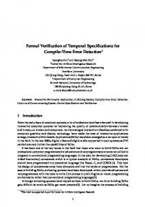
Fig. 2. The sorted doubly-linked list to node-balanced tree method.

Let us consider the method sdl2nbt shown in Fig 2. Taking in a sorted doubly-linked list as argument, sdl2nbt will convert it into a node-balanced tree together with binary search properties, as indicated in lines 2 and 3. Its algorithm proceeds as follows: first it finds the “centre” node in the list (root), where the difference of numbers of its left and right nodes is at most one, as Fig 3 (a) indicates (lines 5-13). Then it applies the algorithm recursively on both list segments on the centre’s left and right hand sides, and regards the centre node as the tree’s root, whose left and right children are the resulted subtrees’ roots from the recursive calls, as in Fig 3 (b) and (c) (lines 14-25). As the data structure of doubly-linked list and binary tree are homomorphic (line 0), we reuse the nodes in the input list instead of creating a new tree, making this algorithm in-place. The parameter head in line 1 denotes the first node of the input list, and tail is where the list’s last node’s next field points to. When using this method tail should be set as null initially. Our framework allows the user to verify and/or refine a number of properties about this code. Firstly, the transformation of shapes from initial to final states (namely, from a doubly-linked list to a binary tree) must be captured. Secondly, some structural numerical information should be inferred, so as to prove the node counts before and after the method invocation are the same and the node-

10

S. Qin, C. Luo, W.-N. Chin and G. He

d a e h l l u n

t o o r 1

2

3

d n e 4

5

6

l i a t

(a) t o o r

t o o r 4

4

2 1

6 3

5 (b)

2 1

6 3

5 (c)

Fig. 3. Transferring from a sorted doubly-linked list to a node-balanced BST.

balanced property of the tree, etc. Meanwhile, we also want to derive relational numerical information as lists’ sortedness and trees’ binary search property, and finally set/bag information like the symbolic content of the list’s and the tree’s (in order to prove the values stored in the list and the resulted tree are the same). Finally, some obligation for memory safety should be found in the precondition, to ensure the input list is non-empty (otherwise the dereference in line 15/17 will fail). To deal with all these properties, we expect the user to provide shape information for primary methods’ specifications as in Fig 2. Based on that, we try to compute the remaining constraints (including the missing parts of pure specifications for primary methods, and both pre- and post-conditions for loops and auxiliary methods). As for the example, as the user has provided the pre- and post-shapes for method sdl2nbt, our analysis proceeds in two steps: generating the constraint abstraction, and solving it. The first step is mainly a symbolic execution over the program to find its postcondition, so as to generate the constraint abstraction. During this step, for any loops and/or auxiliary method calls (lines 7-13 in the example), the symbolic execution will invoke the analysis procedure again to compute their specifications for the current execution to continue (Section 2.5). Therefore we can find the while loop’s postcondition as head::sdlBhnull, root, Sh i ∗ root::sdlBhp, tail, Sr i ∧ end=tail ∧ S=Sh ⊔Sr ∧ (∀x∈Sh , y∈Sr ·x≤y) ∧ 0≤|Sh |−|Sr |≤1

(5)

which indicates that the original list segment starting from head is cut into two pieces with a cutpoint root, where both are still sorted and the content is also preserved. Meanwhile, the essential constraint (the underlined part, saying the

Automatically Refining Partial Specifications for Program Verification

11

list beginning with head is at most one node longer than that with root) to ensure the node-balanced property is derived as well. When the symbolic execution finishes, it generates the following constraint abstraction as the postcondition of the method: Q(head, p, q, S, res, Sres ) ::= root::node2hv, null, nulli ∧ head=root=res ∧ tmp=q=tail ∧ p=null ∧ S={v} ∨ head::node2hs, null, rooti ∗ root::node2hv, resh , nulli ∧ res=root ∧ tmp=q=tail ∧ p=null ∧ S={s, v} ∧ s≤v ∨ resh ::nbthShres i ∗ resr ::nbthSrres i ∗ root::node2hv, resh , resr i ∧ P(head, p, root, Sh , resh , Shres ) ∧ P(tmp, null, tail, Sr , resr , Srres ) ∧ head6=root ∧ root=res ∧ tmp6=tail ∧ q=tail ∧ S=Sh ⊔{v}⊔Sr ∧ (∀x∈Sh , y∈Sr ·x≤v≤y) ∧ 0≤|Sh |−|Sr |≤1 where P stands for corresponding pure constraint abstraction explained below. The first two disjunctive branches are base cases of the method’s invocation, and the last denotes the effect of recursive calls combined into the postcondition. The first case represents the scenario where there is only one node in the original list (with res as the method’s return value). The second is for the case of two nodes, one referenced by head, pointing to the other one, root. In this case the value of head is no more than that of root. The third case is defined recursively with the constraint abstraction itself, meaning that the post-state concerns the root node and the post-states of two recursive calls over head and tmp, respectively. Note that Sres does not appear in Q’s definition. Since it stands for pure properties in user-provided post-shape, it will be involved when we abstract Q against that post-shape in the next step. The second step solves the constraint abstraction Q by finding a closed-form approximation of it. Instead of performing a fixpoint analysis directly on Q over the combined domain, we first derive a pure constraint abstraction P (with the help of Sleek) from Q and the user-provided heap part of postcondition. Then we are able to use some existing conventional solvers [36, 38] to compute the pure fixpoint. For the sdl2nbt method, we generate the pure constraint abstraction P based on the following entailment relation: Q(head, p, q, S, res, Sres ) ⊢ res::nbthSres i ∧ P(head, p, q, S, res, Sres ) which produces the following pure constraint abstraction P: P(head, p, q, S, res, Sres ) ::= head=root=res ∧ tmp=q=tail ∧ p=null ∧ S=Sres ={v} ∨ head6=root ∧ res=root ∧ tmp=q=tail ∧ p=null ∧ S=Sres ={s, v} ∧ s≤v ∨ P(head, p, root, Sh , resh , Shres ) ∧ P(tmp, null, tail, Sr , resr , Srres ) ∧ head6=root ∧ root=res ∧ tmp6=tail ∧ q=tail ∧ S=Sh ⊔{v}⊔Sr ∧ Sres =Shres ⊔{v}⊔Srres ∧ (∀x∈Sh , y∈Sr ·x≤v≤y) ∧ 0≤|Sh |−|Sr |≤1

12

S. Qin, C. Luo, W.-N. Chin and G. He

Note that the heap information is already eliminated from P; instead the constraints over Sres are included during the entailment checking procedure. This allows us to solve P to refine the user-provided shape-only specification. After solving P, we achieve the following constraint: p=null ∧ q=tail ∧ S=Sres ∧ |S|≥1 with which we can refine the method’s specifications as requires head::sdlBhp, q, Si ∧ p=null ∧ q=tail ∧ |S|≥1 ensures res::nbthSres i ∧ S=Sres which proposes more requirements in the precondition, as the head’s prev field should be null, and the whole list’s last node’s next field must point to tail. Meanwhile, there should be at least one node in the list for the sake of memory safety. With those obligations, the method guarantees that the result is an nodebalanced tree with binary search property, whose content is the same as the input list. 2.5

Analysis for the While Loop in Example

In the method sdl2nbt, there is a while loop (lines 7-13) to discover the centre node of the given list segment referenced by head. It traverses the list segment with two pointers root and end. The end pointer goes towards the list segment’s tail twice as fast as root. When end arrives at the tail of the segment (tail), root will point to the list segment’s centre node. As we want to minimise user’s annotations, we do not require the user to supply loop invariant; instead we will try to calculate its postcondition. As aforementioned, our analysis must first synthesise its pre- and post-states with shape information, and then proceed with its constraint abstraction. For pre it is straightforward as the program state before the loop will provide relevant shape information. For post it is done by checking the loop body (unrolled once)’s symbolic execution result against all possible abstracted shapes. For the previous example, we first generate all possible shapes according to the variables accessed by the loop, such as (a) head::sdlBhph , qh , Sh i ∗ root::sdlBhpr , qr , Sr i, and (b) head::sdlBhph , qh , Sh i ∗ root::nbthhr , br , Sr i, and many so forth. Then the unrolled loop body is symbolically executed several times to filter out any invalid shape as an invariant. In the example’s case, executing the loop body will yield the following result: head::node2hv, p, endi ∧ head=root ∧ end=tail ∨ head::node2hvh , p, rooti ∗ root::node2hvr , head, endi ∧ end=tail

(6)

where (b) is directly filtered out since (6) ⊢ (b) ∗ true fails. However (a) remains a candidate, as both (6) ⊢ (a) ∗ true holds. Therefore, regarding (a) as a possible shape post, we can employ the same approach for the whole method to generate

Automatically Refining Partial Specifications for Program Verification

13

a constraint abstraction for the while loop, and solve it to achieve formula (6) in the last section. One more note for the while loop in this example is that the symbolic execution may actually permit more than one shapes to enter as candidates, e.g. head::sdlBhph , qh , Sh i. Generally this does not affect the analysis result, as we allow the analysis to continue with all possible postconditions computed from this while loop, and always choose the most precise final result. In the motivating example, both head::sdlBhph , qh , Sh i and (a) are valid shape postconditions for the loop, but later the former one will cause the analysis to fail in line 15/17, because it inappropriately approximated the invariant and hence lost information about root. Since we synthesise all possible shapes, we can always select those shapes sufficiently strong to support further analysis to obtain a meaningful result.

3

Language and Abstract Domain

To simplify presentation, we focus on a strongly-typed C-like imperative language in Fig 4. A program Prog consists of type declarations tdecl, which can define either data type datat (e.g. node) or predicate spred (e.g. llB), and some method declarations meth. The definitions for spred and mspec are given later in Fig 5. The language is expression-oriented, so the body of a method is an ex-

Prog datat meth e d d[v]

::= tdecl∗ meth∗ tdecl ::= datat | spred | lemma ::= data c { field∗ } field ::= t v t ::= c | τ ::= t mn ((t v)∗ ; (t v)∗ ) mspec∗ {e} τ ::= int | bool | void ::= d | d[v] | v=e | e1 ; e2 | t v; e | if (v) e1 else e2 | while (v) {e} ::= null | kτ | v | new c(v ∗ ) | mn(u∗ ; v ∗ ) ::= v.f | v.f :=w | free(v) Fig. 4. A Core (C-like) Imperative Language.

pression composed of e (the recursively defined program constructor) and d and d[v] (atom instructions). We also allow both call-by-value and call-by-reference method parameters (which are separated with a semicolon ;where the ones before ; are call-by-value and the ones after are call-by-reference). Our specification language (in Fig 5) allows (user-defined) shape predicates to specify both separation and pure properties. The shape predicates spred and lemmas lemma are constructed with disjunctive constraints Φ. We require that the predicates be well-formed [35]. A conjunctive abstract program state, σ, is composed of a heap (shape) part κ and a pure part π, where π consists of γ, φ and ϕ as aliasing, numerical and bag information, respectively. We use SH to denote the set of such conjunctive states. During the symbolic execution, the abstract program state at each program point will be a disjunction of σ’s, denoted by ∆. Note that constraint abstractions (e.g. Q(v∗ )) may occur in ∆ during the analysis.

14

S. Qin, C. Luo, W.-N. Chin and G. He spred mspec ∆ Φ Υ κ ω γ φ b s ϕ B

::= pred(v ∗ ) ≡ Φ lemma ::= pred(v ∗ ) ∧ π ←− Φ ::= requires Φpr ensures Φpo ∗ ::= Q(v W ∗) | Φ | ∆1 ∨∆2∗ | ∆∧π | ∆1 ∗∆2 | ∃v·∆ ::= σ ∃v ·κ∧π Wσ ::= ::= P(v ∗ ) | ω ∗ | Υ1 ∧Υ2 | Υ1 ∨Υ2 | ∃v·Υ ::= emp | v7→c(v ∗ ) | pred(v ∗ ) | κ1 ∗ κ2 ::= ∃v ∗ ·π π ::= γ∧φ ::= v1 =v2 | v=null | v1 6=v2 | v6=null | γ1 ∧γ2 ::= ϕ | b | a | φ1 ∧φ2 | φ1 ∨φ2 | ¬φ | ∃v · φ | ∀v · φ ::= true | false | v | b1 = b2 a ::= s1 =s2 | s1 ≤s2 ::= kint | v | kint ×s | s1 +s2 | −s | max(s1 ,s2 ) | min(s1 ,s2 ) | |B| ::= v∈B | B1 =B2 | B1 1}, we have the following reasoning procedure: {x′ =x ∧ x>1} x:=x+1 {x>1 ∧ x′ =x+1} x:=x-2 {x>1 ∧ x′ =x1 −2 ∧ x1 =x+1} where the final value of x is recorded in variable x′ and x1 keeps an intermediate state of x.

Automatically Refining Partial Specifications for Program Verification

4

15

The Analysis

The overall algorithm is listed in Fig 6.

Algorithm Analysis(T , S, mn, σ, x∗ , y ∗ ) 1 case mn of 2 | while (w) {e0 } → f := fresh name(); e := if (w) {e0 ; f (x∗ ; y ∗ )}; ! (u∗ , v ∗ ) := (x∗ , y ∗ ); ([(Φipr , Φipo )], n) := Preproc(T , S, f, x∗ , y ∗ , e0 , σ, x∗ , y ∗ ); ! prim := false; 3 | t mn ((t u0 )∗ ; (t v0 )∗ ) {e0 } → f := mn; e := e0 ; (u∗ , v ∗ ) := (u∗0 , v0∗ ); ! ([(Φipr , Φipo )], n) := Preproc(T , S, f, u∗ , v ∗ , e0 , σ, x∗ , y ∗ ); prim := false; po m 4 | t mn ((t u0 )∗ ; (t v0 )∗ ) (requires Φpr i ensures Φi )i=1 {e0 } → f := mn; po m ∗ ∗ ∗ ∗ i i m ! e := e0 ; (u , v ) := (u0 , v0 ); n := m; (Φpr , Φpo )i=1 := (Φpr i , Φi )i=1 ; ! prim := true; 5 end case 6 sps := ∅ 7 for i := 1 to n do 8 sp := CA Gen Solve(T , f, e, Φipr , Φipo , u∗ , v ∗ ) 9 if prim = false and sp 6= fail then return (f, sp) 10 else if prim = true then sps := sps ∪ sp 11 end if 12 end for 13 return (f, sps) end Algorithm

Fig. 6. Main analysis algorithm.

Our analysis algorithm takes as input all available specifications and shapes, and the code segment to be analysed, together with an optional conjunctive program state and two variable sequences (mainly for loops and auxiliary methods). The algorithm first recognises the type of input code segment (mn in line 1). In the first two cases (while loop in line 2 and auxiliary method call in line 3), we do not know anything about the code’s specifications; therefore some preprocessing should be done to discover the code’s pre- and post-shapes with Preproc (Fig. 7). For primary method (line 4), as the user should have provided the shape-based specifications, no preprocessing is needed. Then the constraint abstraction generation and solving algorithm is applied to each specification to refine it (line 8). Note here we apply a lazy scheme for loops and auxiliary methods: as the pre-processing may yield several possible shape specifications in a list (ordered with heuristics such that the specifications with more possibility to make the whole verification succeed are more in front), we try to verify each in sequence. Once a specification can be verified against the program, then it is returned and the other ones are omitted. In this way we try to make our verification more scalable, as still will be described in later sections.

16

S. Qin, C. Luo, W.-N. Chin and G. He Algorithm Preproc(T , S, f, u∗ , v ∗ , e, σ, x∗ , y ∗ ) 1 sps := [ ]; 2 prs := SynPre(S, f, u∗ , v ∗ , σ, x∗ , y ∗ ) 3 for Φpr ∈ prs do 4 pos := SynPost(T , S, f, e, Φpr , u∗ , v ∗ ) 5 sps := concat(sps, pos) 6 end for 7 return (sps, |sps|) end Algorithm Fig. 7. Pre-processing algorithm.

The pre-processing algorithm mainly invokes the shape synthesis procedures to discover all possible pre- and post-shapes for loops and auxiliary methods, as shown in lines 1 and 4. Then the list of shape pairs (specifications) are returned and used in further analysis. The details of shape synthesis algorithms will be introduced in Section 4.3.

4.1

Refining Specifications for Primary Methods

The algorithm for refinement (CA Gen Solve) is given in Fig 8. As illustrated in Section 2.2, the analysis proceeds in two steps for a primary method with shape information given in specification, namely (1) forward analysis (at lines 1-2) and (2) pure constraint abstraction generation and solving (at lines 3-10).

Algorithm CA Gen Solve(T , mn, e, Φpr ,Φpo ,u∗ ,v ∗ ) 1 ∆ := Symb Exec(T , mn, e, Φpr ) 2 if ∆ = fail then return fail end if W 3 Normalise ∆ to DNF, and denote as m i=1 ∆i ∗ ∗ ∗ ′∗ ∗ ∗ ′∗ 4 w :={u ,v ,v } ∪ pureV({u ,v ,v }, Φpr ∨Φpo ) W 5 ∆P := Pure CA Gen(Φpo , Q(w∗ )::= m i=1 ∆i ) 6 if ∆P = fail then return fail end if 7 π := Pure CA Solve(P(w∗ )::=∆P ) 8 R := t mn ((t u)∗ ; (t v)∗ ) requires ! ex quan(Φpr , π) ensures ex quan(Φpo , π) 9 if Verify(T , mn, R) then return T ∪ {R} \ ! { t mn ((t u)∗ ; (t v)∗ ) requires Φpr ensures Φpo } 10 else return fail end if end Algorithm

Algorithm Symb Exec ! (T , mn, e, Φpr ) 11 errLbls := ∅ 12 do 13 (∆, l) := |[e]|mn T (Φpr , 0) 14 if l>0∧l∈errLbls / then 15 Φpr :=ex quan(Φpr ,∆); 16 errLbls := errLbls ∪{l} 17 else if l>0 ∧ l∈errLbls ! then return fail 18 end if 19 while l > 0 20 return ∆ end Algorithm

Fig. 8. Refining method specifications.

Automatically Refining Partial Specifications for Program Verification

17

The forward analysis is captured as algorithm Symb Exec to the right of Fig 8. Starting from a given pre-shape Φpr , it analyses the method body e to compute the post-state in constraint abstraction form. The symbolic execution rules are given in the appendix. They are similar to symbolic rules used in [35, 39], except for a novel mechanism to derive pure precondition, which we refer to as pure abduction. This pure abduction mechanism is invoked whenever symbolic execution fails to prove memory safety based on the current prestate. For example, if we have ll(x, n) as the current state and we require x7→node( , p) to update the value of p, then it will fail as ll(x, n) does not necessarily guarantee x7→node( , p). In this case we conduct the pure abduction as ll(x, n) ∧ [n≥1]  x7→node( , p) ∗ true to compute the missing pure information (in the squared bracket) such that the LHS (including the newly gained pure part) entails the RHS. The variable errLbls (initialised at line 11) is to record the program locations in which previous pure abductions occurred. Whenever the symbolic execution fails, it returns a state ∆ that contains the pure abduction result and the location l where failure was detected, as shown in line 13. If the current abduction location l is not recorded in errLbls, it indicates that this is a new failure. The abduction result is added to the precondition of the current method to obtain a stronger Φpr , before the algorithm enters the symbolic execution loop with variable errLbls updated to add in the new failure location l. This loop is repeated until symbolic execution succeeds with no memory error, or a previous failure point was re-encountered. The latter indicates either a program bug or a specification error. For example, for a method void foo (...) {node w := new node(0, null); goo(w); ...} invoking a method goo(x) with precondition ll(x, n)∧n≥2, our analysis will perform an abduction to get n≥2 since it is not implied by the current state. However, as n is for the shape of local variable w, it will be quantified away when propagating n≥2 back, ending up with true being added to foo’s precondition. In the next round of symbolic execution, our analysis will have the same abduction at the same point. Back to the main algorithm CA Gen Solve, the analysis next builds a heapbased constraint abstraction mechanism, named Q(w∗ ), for the post-state in steps 3-4. This constraint abstraction is possibly recursive. (Definition † in page 5 is an example of this heap-based abstraction.) We then make use of another algorithm in Fig 9, named Pure CA Gen, to extract a pure constraint abstraction, named P(w∗ ), without any heap property. (Definition ‡ in page 6 is an instance of this pure abstraction.) This algorithm tries to derive a branch Pi for each branch ∆i of Q. For every ∆i it proceeds in two steps. In the first step (lines 22-24), it replaces the recursive occurrence of Q in ∆i with σ ∗ P(w∗ ). In the second step (lines 25-26) it tries to derive Pi via the entailment. If the entailment fails, then pure abduction is used to discover any missing pure constraint σi′ for ρ∆i to allow the entailment to succeed. In this case, σi′ is incorporated into σi (and eventually Pi ). Once this is done, we use some existing fixpoint analysis (e.g. [38]) inside

18

S. Qin, C. Luo, W.-N. Chin and G. He

Pure CA Solve to derive non-recursive constraint π, as a simplification of P(w∗ ). This result is then incorporated into the pre/post specifications in line 8, before we perform a post verification in line 9 using the Hip verifier [35], to ensure the strengthened precondition is strong enough for memory safety. Two auxiliary functions used in the algorithm are described here. The function pureV(V, ∆) retrieves from ∆ the shapes referred to by all pointer variables from V , and returns the set of logical variables used to record numerical (size and bag) properties in these shapes, e.g. pureV({x}, ll(x, n)) returns {n}. This function is used in the algorithm to ensure that all free variables in Φpr and Φpo are added into the parameter list of the constraint abstraction Q. The function ex quan(∆, π) is to strengthen the state ∆ with the abduction result π: ex quan(∆, π) =df ∆ ∧ ∃(fv(π) \ fv(∆)) · π. It is used to incorporate the discovered missing pure constraints into the original specification. For example, ex quan(ll(x, n), 0 0

f |[d[x]]|T (∆, 0) f |[d]|T (∆, 0) f |[e1 ; e2 ]|T (∆, 0)

=df exec† (d[x])(T ,f )(unfold† (x)∆, 0) =df exec† (d)(T ,f )(∆, 0) f

f

=df |[e2 ]|T ◦ |[e1 ]|T (∆, 0) f

f

|[v := e]|T (∆, 0) =df [v1 /v ′ , r1 /res](|[e]|T (∆, 0)) ∧ v ′ =r1 , fresh v1 , r1 f

f

(∆′2 , l2 ) = |[e2 ]|T (¬v∧∆, 0)

(∆′1 , l1 ) = |[e1 ]|T (v∧∆, 0) f

|[if (v) e1 else e2 ]|T (∆, 0) =df (∆′1 ∨ ∆′2 , max{l1 , l2 })

B

Soundness

This section proves the lemmas and theorem for soundness in Section 4. f

Lemma 1 (Sound abstract semantics). If |[e]|T (∆, 0) = (∆1 , 0), then for all s, h, if s, h |= ∆ and hs, h, ei֒→hs1 , h1 , e1 i, then there always exists ∆0 such that s1 , h1 |= ∆0

and

f

|[e1 ]|T (∆0 , 0) = (∆1 , 0)

Automatically Refining Partial Specifications for Program Verification

Proof

31

The proof is done by structural induction over program constructors:

– Case null | k | v | v.f . Straightforward. – Case v := e. There are two cases according to the operational semantics: • e is not a value. From operational semantics, there is e1 s.t. hs, h, ei֒→hs1 , h1 , e1 i, and hs, h, v:=ei֒→hs1 , h1 , v:=e1 i. From abstract semantics for asf signment, if |[e]|T (∆, 0) = (∆2 , 0), and ∆1 =[v1 /v ′ , r1 /res](∆2 )∧v ′ =r1 . f By induction hypothesis, there exists ∆0 , s1 , h1 |= ∆0 and |[e1 ]|T (∆0 , 0) = f (∆2 , 0). It concludes from the assignment rule that |[v := e1 ]|T (∆0 , 0) = (∆1 , 0). • e is a value. Trivial. – Case v1 .f := v2 . Take S0 = S. It concludes immediately from the exec rule for field update and the underlying operational semantics. f – Case new c(v ∗ ). From abstract semantics for new, we have |[new c(v ∗ )]|T (∆, 0) = (∆1 , 0), where ∆1 = ∆ ∗ c(res, v1′ , .., vn′ ). Let ∆0 = ∆1 . From the operational semantics, we have hs, h, new c(v ∗ )i֒→hs, h+[ι 7→ r], ιi, where ι ∈ / dom(h). From f s, h |= ∆, we have s, h+[ι 7→ r] |= ∆0 . Moreover, |[ι]|T (∆0 , 0) = (∆1 , 0). – Case e1 ; e2 . We consider the case where e1 is not a value (otherwise it is straightforward). From the operational semantics, we have hs, h, e1 i֒→hs1 , h1 , e3 i. From the abstract semantics rule for sequence, we have ⊢ {∆}e1 {∆2 }. By induction hypothesis, there exists ∆0 s.t. s1 , h1 |= Post(∆0 ), and ⊢ {∆0 }e3 {∆2 }. f By the sequential rule we have |[e3 ; e2 ]|T (∆0 , 0) = ∆1 . – Case if (v) e1 else e2 . There are two possibilities in the operational semantics: • s(v)=true. We have hs, h, if (v) e1 else e2 i֒→hs, h, e1 i. Let ∆0 = (∆∧v ′ ). It is obvious that s, h |= ∆0 . From the if-conditional rule of abstract semantics, we have: f |[e1 ]|T (∆0 , 0) = (∆2 , 0) f |[e2 ]|T (∆∧¬v ′ , 0) = (∆3 , 0) And we also have (due to sound weakening of postcondition) f

|[e1 ]|T (∆0 , 0) = (∆2 ∨∆3 , 0) f

That is, |[e1 ]|T (∆0 , 0) = (∆1 , 0). • s(v) = false. Analogous. – Case mn(v1..n ). For the method invocation rule, we know ∆⊢[vj′ /vj ]nj=1 Φipr ∗ ∆i , Wp for i = 1, .., p. Take ∆0 = i=1 [vj′ /vj ]nj=1 Φipr ∗∆i . From the operational semantics and the above heap entailment, we have s1 , h1 |= ∆0 . Then the f method invocation rule implies ∀i∈1..p · |[e1 ]|T ([vj′ /vj ]nj=1 Φipr ∗∆i , 0) = (∆i ∗Φipo , 0). f Therefore we have |[e1 ]|T (∆0 , 0) = (∆1 , 0) which concludes. – Case while (v) {e}. It can be converted to tail-recursive method call with all parameters passed by reference, and thus follows the above case. 2

32

S. Qin, C. Luo, W.-N. Chin and G. He

Lemma 2 (Sound pure constraint abstraction). Given a method with pre/post shape templates pre and post, if our analysis successfully computes a constraint abstraction Q in the first step, and derives a pure constraint P in the second step, then we have Q ⊢ post ∧ P. Proof This proof follows directly our procedure to compute the pure constraint abstraction from the shape one. Denote the shape constraint abstraction as _ Q ::= Qi i

and the provided post-shape post, we use Qi ⊢ post ∧ Pi to derive each Pi , and construct P ::=

_

Pi

i

Therefore, W our result Q ⊢ post ∧ P can be obtained from the fact that post ∧ ( i Pi ).

W

i

Qi ⊢ 2

Theorem 2 (Soundness). Our analysis is sound with respect to the underlying operational semantics. Proof For a method t mn ((t u)∗ ; (t v)∗ ) requires Φpr ensures Φpo {e}, suppose we have the resulted pure constraint π. Then, for all s, h |= Φpr ∧ ex quan(Φpr , π) mn and |[e]|T (ΦprW ∧ ex quan(Φpr , π), 0) = (∆, 0), Wwe know s′ , h′ |= ∆ (Lemma 1). Thus let ∆ = Qi , we have s′ , h′ |= lfix λ Q. Qi where lfix is the least fixedpoint operator. Then due of entailment, we know W to Lemma 2 and the soundness W s′ , h′ |= Φpo ∧ lfix λ P. Pi . Because π = lfix λ P. Pi , we can claim s′ , h′ |= Φpo ∧ π. Finally from the definition of ex quan(Φpo , π) (as its result is a weakening of π by quantifying out its local variables) we know s′ , h′ |= Φpo ∧ ex quan(Φpo , π). 2

Automatically Refining Partial Specifications for Program Verification Prog. Time Pre List processing programs 0.379 emp ∧ n≥0

33

Post llB(res, S) ∧ n=|S| ∧ ∀v∈S·1≤v≤n

1.752 emp ∧ n≥0

dllB(res, rp, S) ∧ n=|S| ∧ ∀v∈S·1≤v≤n

0.954 emp ∧ n≥0

sllB2(res, S) ∧ n=|S| ∧ ∀v∈S·1≤v≤n

0.591 ll(x, n) ∧ n≥1 0.789 dll(x, p, n) ∧ n≥1

ll(x, m) ∧ m=n+1 dll(x, q, m) ∧ n≥1 ∧ m=n+1 ∧ p=q

0.504 sll(x, n, xs, xl)∧ v≥xs

sll(x, m, mn, mx)∧ xs=mn∧mx=max(xl,v)∧m=n+1

tail insert

0.566 ll(x, n) ∧ n≥1 0.628 sll(x, n, xs, xl)∧ v≥xl

ll(x, m) ∧ m=n+1 sll(x, m, mn, mx) ∧ v=mx ∧ mn=xs ∧ m=n+1

rand ∗ insert

0.522 ll(x, n) ∧ n≥1 0.830 dll(x, p, n) ∧ n≥1

ll(x, m) ∧ m=n+1 dll(x, q, m) ∧ m=n+1 ∧ p=q

∗

create

sort ∗ insert

— delete delete

sll(x, n, xs, xl)∧ (fail)

0.630 llB(x, S) ∧ |S|≥2

llB(x, T) ∧ ∃a.S=T⊔{a}

1.024 sllB(x, S) ∧ |S|≥2

sllB(x, T) ∧ ∃a.S=T⊔{a}

1.252 dllB(x, p, S) ∧ |S|≥2

dllB(x, q, T) ∧ ∃a.S=T⊔{a} ∧ p=q

0.296 ll(x, m)∧ n≥0∧m≥n

ls(x, p,k)∗ll(res, r)∧ p=res∧k=n∧m=n+r

travrs 2.205 sllB(x, S) ∧ n≥0∧|S|≥n 0.512 ll(x, xn)∗ll(y, yn)∧ xn≥1 dll(x, xp, xn) ∗ append∗ 0.660 dll(y, yp, yn) ∧ xn≥1 sll(x, xn, xs, xl)∧ xl≤ys 0.948 ∗ sll(y, yn, ys, yl) Sorting (main) llB(x, S) ∧ |S|≥1 merge

sll(x, m, mn, mx)∧ (fail)

4.107 sllB(x, Sx ) ∗ sllB(y, Sy )

slsB(x, p, T) ∗ sllB(res, S2 )∧ p=res∧|T|=n ∧ S=T⊔S2 ∧ ∀u∈T,v∈S2 · u≤v ll(x, m) ∧ m=xn+yn dll(x, q, m) ∧ m=xn+yn ∧ q=xp sll(x, m, rs, rl) ∧ yl=rl ∧ m≥1+yn ∧ m=xn+yn sllB(res, T) ∧ T=S

(⋆)

sllB(res, T) ∧ T=Sx ⊔Sy sllB(res, T) ∧ T=S

flatten 2.693 bstB(x, S) insert

0.824 sllB(r, S) ∗ x7→node(v, )

sllB(res, T) ∧ T=S⊔{v}

quick

2.132 lbd(x, S)

height insert

0.913 bt(x, S, h) 1.276 bt(x, S, h) ∧ |S|≥1 ∧ h≥1

bt(x, T, k) ∧ res=h=k ∧ S=T bt(x, T, k) ∧ T=S⊔{v} ∧ h≤k≤h+1

delete

0.970 bt(x, S, h) ∧ |S|≥2 ∧ h≥2

bt(x, T, k) ∧ ∃a.S=T⊔{a} ∧ h−1≤k≤h

search

1.583 bst(x, sm, lg)

bst(x, mn, mx) ∧ sm=mn ∧ lg=mx ∧ 0≤res≤1

bst insert

1.720 bst(x, sm, lg)

lbd(x, S1 ) ∗ lbd(res, S2 ) ∧ S=S1 ⊔S2 ∧

∀u∈S1 ∀v∈S2 · u≤p≤v Binary tree, binary search tree, AVL tree and red-black tree processing programs travrs 0.532 bt(x, S, h) bt(x, T, k) ∧ S=T ∧ h=k count 0.709 bt(x, S, h) bt(x, T, k) ∧ res=|S| ∧ S=T ∧ h=k

rbt(res, T) ∧ T=S⊔{v}

8.76 rbt(x, S)

sdl2nbt 5.826

lg