Automorphisms and Encoding of AG and Order Domain Codes John B. Little Department of Mathematics and Computer Science College of the Holy Cross Worcester, MA 01610 USA
[email protected] June 25, 2007 Abstract We survey some encoding methods for AG codes, focusing primarily on one approach utilizing code automorphisms. If a linear code C over Fq has a finite abelian group H as a group of automorphisms, then C has the structure of a module over a polynomial ring P. This structure can be used to develop systematic encoding algorithms using Gr¨obner bases for modules. We illustrate these observations with several examples including geometric Goppa codes and codes from order domains.
1
Introduction
In order for a code to be useful in practice, it should admit efficient encoding and efficient decoding. Although most of the research effort on algebraic geometric (AG) Goppa codes from curves has focused on the decoding side, several approaches have been considered for encoding as well. In this article we will briefly survey several approaches to encoding these codes. We will then concentrate on a systematic encoding method based on the fact that codes possessing permutation automorphisms have the structure of modules over polynomial rings. This discussion is based on Heegard, Little, 1
and Saints, [HLS], which shows how to use module Gr¨obner bases for such codes to construct encoders. This approach is a direct generalization of the commonly-used polynomial division encoding method for cyclic codes that appears in most textbook treatments of coding theory. The module Gr¨obner basis furnishes an analog of the generator polynomial of a cyclic code (see Theorem 2). This particular connection between encoding and Gr¨obner bases was well-established previously in the case of abelian (m-dimensional cyclic) codes. See, for instance, [PH], section 6.1.6, or Chapter 9 of [CLO]. Since it relies only on the presence of suitable groups of code automorphisms, it applies to many classes of codes, including cyclic, quasi-cyclic, abelian, and many Goppa-type evaluation codes from curves, higher-dimensional varieties, and order domains. In the last three cases, interesting code automorphisms often arise from automorphisms of the underlying algebraic variety (see §6). Some results on implementation of this approach in hardware for the case of codes from the Hermitian curves considered in §7 have been reported by Chen and Lu, [CL]. To conclude this introduction, we note that codes with sufficiently large automorphism groups may also be amenable to permutation decoding. In this decoding method, a fixed collection of code automorphisms is applied to the received word. If the error weight is sufficiently small, at least one of the automorphisms will move the errors out of the information positions. Then the correct information symbols can be re-encoded to accomplish the decoding. Chabanne, [C], has considered this decoding method from the point of view of Gr¨obner bases in the case of abelian codes, and [L1] gives an example for a Hermitian code.
2
Other Encoding Methods for AG Goppa Codes
The most basic encoding method for these codes simply treats them as linear codes and uses matrix multiplication of the information word with any generator matrix G to do the encoding. In the article [MOS], Matsumoto, Oishi, and Sakaniwa propose a faster encoding method for the one-point residue codes CΩ (D, mQ) (and also their dual codes). This method is based on the structure of a special basis {xi ωj : 0 ≤ j ≤ a − 1, vQ (xi ωj ) ≥ m} 2
for the vector space of differentials Ω(mQ − D). Here x is an element of the Riemann-Roch space L(aQ), where a is the smallest pole order of a nonconstant function with poles only at Q. The ωj are differentials in Ω(−∞Q − D) having the maximum valuation at Q among differentials ω such that vQ (ω)−j is divisible by a. The resulting generator matrix G possesses a block factorization that can be exploited to reduce the number of multiplications involved in computing a product of the form xG. This method does not make use of Gr¨obner bases and yields a nonsystematic encoder. More recently, Matsui and Mita, [MM], have described a method combining discrete Fourier transforms (DFT) and Gr¨obner bases that yields a systematic encoder for the CΩ (D, mQ) = CL (D, mQ)⊥ codes from a Ca,b curve. Their method works as follows. A pair (i, j) with 0 ≤ i, j ≤ q − 1 can represent either the monomial xi y j or the point (αi , αj ) where α is a primitive element of the field. For simplicity, assume D is supported at points in (Fq ∗ )2 . Partition the support into two subsets: a set of information positions P 0 of cardinality k, and a set of parity-checks P of cardinality n − k = dim L(mQ), where Q is the point at infinity on the Ca,b curve. A Gr¨obner basis G for the ideal I(P ) is pre-computed. For most choices of P , the monomials in the footprint or Gr¨obner ´escalier are identified with the collection of pairs (i, j) as above with ai + bj ≤ m. To encode a given information word a = (a(i,j) : (i, j) ∈ P 0 ), the DFT A is computed, where A(i,j) = f (αi , αj ) for the polynomial X f (x, y) = a(k, l) xk y l . (αk , αl )∈P 0
The portion of the DFT corresponding to (i, j) with ai + bj ≤ m is then extended to an array A0 for all (i, j) with 0 ≤ i, j ≤ q − 1 by means of the Gr¨obner basis G. The difference array A − A0 represents the DFT of a codeword in CΩ (D, mQ) since its syndromes corresponding to xi y j with ai + bj ≤ m are all zero. Moreover it can be seen that the inverse DFT of A − A0 provides a systematic encoding of the information a.
3
Automorphisms and module structures
We now prepare for another encoding method by introducing some general information on automorphisms of codes and module structures. The symmetric group Sn acts on Fnq by permuting the entries of vectors. A permutation 3
automorphism of a linear code C ⊂ Fnq is an element of Sn that maps the set of codewords to itself. We will only consider code automorphisms of this type in the following. Let C be a code that has a nontrivial abelian group H of automorphisms. For instance, the ordinary cyclic codes and m-dimensional cyclic codes (also known as abelian codes) are well-studied examples. For simplicity of notation, we will usually restrict to the case that H = hσi is cyclic. The generalization to the product of several cyclic groups is essentially immediate. With the restriction to cyclic groups H, cyclic codes are the most basic examples. But note that we do not assume that H acts transitively on the set of codeword components. Hence, for instance, the quasicyclic codes of length n also have this sort of structure (by definition, C is quasicyclic if its automorphism group contains an m-fold cyclic shift for some m dividing n) . Let Oi , i = 1, . . . , r be the orbits of the components of the codewords c under the action of H. Pick any component ci, 0 in the ith orbit and label the components in that orbit as ci, j where j = 0, . . . , | Oi | − 1. With the convention that the second index is an integer modulo | Oi |, the action of σ can be written as σ(ci, j ) = ci, j+1 for all i = 1, . . . , r, and j = 0, . . . , | Oi | − 1. For the remainder of this article, P will denote the polynomial ring in one variable Fq [t]. As usual, let ei be the ith standard basis vector in the free module P r . Then the orbit structure of the components of the codewords of C determines the submodule h(t|Oi | − 1)ei : i = 1, . . . , ri of P r . We can view the code C as subset of the quotient module N = P r /h(t|Oi | − 1)ei : i = 1, . . . , ri,
(1)
via the mapping φ:C → N (ci, j ) 7→
r X i=1
|Oi |−1
X
ci, j tj ei mod h(t|Oi | − 1)ei : i = 1, . . . , ri.
j=0
We have the following theorem describing the structure of the image φ(C). Theorem 1 Let C linear block code over Fq with a cyclic group H of automorphisms and φ, N be as above. Then φ(C) has the structure of a Psubmodule of N . 4
Proof: First φ is linear, so φ(C) is an Fq -vector subspace of N . By the definition of φ, if c ∈ C is any codeword, multiplication of φ(c) by t yields |Oi |−1 r X X t · φ(c) = ci, j tj+1 ei i=1
≡
r X i=1
j=0
|Oi |−1
X
ci, j−1 tj ei mod N
j=0
= φ(σ −1 (c)). By hypothesis, this is another element of φ(C). Hence φ(C) is closed under multiplication by t, hence under multiplication by all polynomials in P. It follows that φ(C) is a P-submodule of N . ¤ Note that if the theorem applies to a code C, it applies to the dual code C ⊥ as well. In [HLS], [LSH], and [L1], this essentially straightforward generalization of the usual construction showing that a cyclic code of length n over Fq is an ideal in P/htn − 1i was applied to some AG Goppa codes. We will present several explicit examples in §7. The article [LF] applies the module structures described here to study quasicyclic codes. Theorem 1 can also be generalized to more general finite abelian automorphism groups. In those cases, we obtain module structures over the polynomial ring in s variables if a minimal generating set for H has s elements.
4
A systematic encoding algorithm
We will now show how the theory of Gr¨obner bases for modules can be applied to work with these codes. Let M(C) be the submodule of P r corresponding to φ(C) ⊂ N under the mapping π : P r → N, where N is the quotient module from (1). The key observation here is that the canonical form algorithm with respect to a Gr¨obner basis G for M(C) with respect to any term ordering ≺ on P r can be used to produce a systematic encoder for C. 5
The encoding algorithm can be described succinctly using the standard and nonstandard terms for M(C). Following the general notational conventions of this volume, N≺ (M(C)) will denote the Gr¨obner ´escalier or “footprint” of the module M(C) with respect to a term order ≺. Similarly, T≺ (M(C)) will denote the leading term module of M(C). The terms tj ei ∈ N≺ (M(C)) will be called the standard terms. The nonstandard terms are the tj ei with j ≤ | Oi | − 1 contained in T≺ (M(C)). In this method, the coefficients of the nonstandard terms give the information positions in the codewords, and the coefficients of the standard terms are the parity checks. The precise statement of the encoding method is given in the following theorem. Theorem 2 Let G be a Gr¨obner basis for the module M(C) with respect to a term ordering ≺ on P r . The algorithm below produces a codeword c in all cases and gives a systematic encoder for the code C. Input: G, the nonstandard terms mi , information symbols ci Output: c, a codeword P f= ci mi ; c := f − CanonicalForm(f, G); Proof: Since CanonicalForm(c) = CanonicalForm(f −CanonicalForm(f, G), G) = 0, it follows that c ∈ M(C), which means that c represents a codeword of C. The information symbols appear as coefficients of the nonstandard terms in f , but CanonicalForm(f, G) is a linear combination of standard terms. The sets of nonstandard and standard terms are disjoint, hence this encoder is systematic, in the sense that the information symbols appear unchanged in a subset of the codeword entries. ¤ Some important examples of the term orderings that can be used here are obtained as follows. First order the ej themselves; we will use e1 > e2 > · · · > er ,
6
but the opposite order is also possible and is used too. The position over term (or P OT ) ordering on P r is defined by ti ej ≺P OT tk e` if j > `, or j = ` and i < k. Reversing the way the comparison is made, we obtain the term over position (or T OP ) ordering on P r : ti ej ≺T OP tk e` if i < k, or i = k and j > `.
5
Complexity Comparisons
The basic encoding method described at the start of §2 requires kn products and (k − 1)n sums in Fq to compute the matrix product xG if G is a general, dense generator matrix. By way of comparison, the method of [MOS] described in §2 effectively reduces the storage space and the number of operations needed. However, as noted above, this encoding method is not systematic. One potential advantage of exploiting the module structures described in Theorem 1 is that, as is true for the generator polynomial of a cyclic code, a Gr¨obner basis for M(C) is typically significantly smaller than a full systematic generator matrix. The exact savings in stored information (or the size of the circuit in hardware) required for the encoding depends on the particular code. However, the situation in Example 2 in §7 below is quite typical. The code C there is a [64, 44, 8] code over F8 . A reduced echelon form systematic generator matrix would be a 44 × 64 matrix G = (I|X) with X a 44 × 20 block of potentially nonzero entries. The Gr¨obner basis for the module M(C) has 10 generators, which contain at most 5 × 2 + 6 × 4 + 7 × 6 + 8 × 7 + 9 = 141 nonzero, non-leading terms. The division algorithm used for encoding in Theorem 2 takes roughly the same amount of arithmetic as the matrix product xG (see [HLS]). The authors of [MM] conjecture that their method requires less field arithmetic than multiplication xG with a systematic generator matrix but do not prove this. The Gr¨obner basis for the ideal I(P ) would typically be even smaller than the Gr¨obner basis for the module M(C) when there is a module structure. 7
6
Automorphisms of curves and AG Goppa codes
In [HLS], it was pointed out that many examples of AG Goppa codes have the module structures described in Theorem 1, hence systematic encoders as described in Theorem 2, because of the presence of automorphisms of the underlying curves. Indeed, many interesting curves with large numbers of Fq -rational points also tend to have large automorphism groups. Let X be a smooth projective algebraic curve defined over Fq . An automorphism of X is a regular mapping from X to itself with a regular inverse. An automorphism σ of X defined over Fq induces an Fq -automorphism of the function field K = Fq (X ) (an isomorphism of fields from K to itself that is the identity on Fq ) via f 7→ f ◦ σ −1 . The set of all automorphisms of X forms a group Aut(X ) under function composition and Aut(X ) acts on divisors on P P X in the obvious way: σ( nP P ) = nP σ(P ). In fact, all of the examples of automorphisms we will consider will be induced by invertible linear mappings on the ambient projective space of X . If such a mapping takes the curve X to itself, then it induces an automorphism of X . For instance, consider the Hermitian function fields and curves over Fq2 . The Hermitian curve may be defined as the variety 2 V(xq+1 + xq+1 + xq+1 0 1 2 ) ⊂ P ,
where (x0 : x1 : x2 ) is the homogeneous coordinate vector of a point in P2 . In section VI.3 of [S], it is shown that (in geometric language) the tangent line to this curve at an Fq2 -rational point can be taken to the line at infinity by a linear change of coordinates in P2 . When that is done, the defining equation is taken to the form given in the following HC q = V(xq+1 − y q z − yz q ) = {(x : y : z) ∈ P2 : xq+1 − y q z − yz q = 0}. (2) We will use this form of the equations of the Hermitian curves. Let α be a primitive element of Fq2 . The mapping σ : P2 → P2 (x : y : z) 7→ (αx : αq+1 y : z)
(3)
induces an automorphism of the curve HC q because it is easy to check that if the point (x : y : z) satisfies the equation in (2), the same is true of σ(x : y : z). 8
In the construction of an AG Goppa evaluation code on P a curve X , ren call that one begins by selecting Fq -rational divisors D = i=1 Pi and E with disjoint supports on X . The codewords are obtained by evaluating the rational functions f in the vector space L(E) = {f : (f ) + E ≥ 0} ∪ {0} at the points in D: ev : L(E) → Fnq f 7→ (f (P1 ), . . . , f (Pn )). The image of the evaluation mapping is the AG Goppa evaluation code CL (D, E). Theorem 3 In this situation, let σ be an automorphism of the curve X and assume the divisors D and E are fixed by σ. Then σ induces an automorphism of the code CL (D, E). Proof: Since σ fixes the divisor E, it follows that f 7→ f ◦ σ −1 takes L(E) to itself. Hence we can define an action of σ on the codewords of CL (D, E) by (f (P1 ), . . . , f (Pn )) 7→ (f (σ −1 (P1 )), . . . , f (σ −1 (Pn ))). Since the divisor D is also assumed to be fixed by σ, this means that the points {σ −1 (Pi )} are a permutation of the {Pi }. Hence σ induces a permutation automorphism of the code CL (D, E). ¤ By Proposition VII.3.3 of [S], the subgroup hσi of Aut(X ) can be viewed as a subgroup of the permutation automorphism group of CL (D, E) whenever n > 2g + 2, where g is the genus of X . Furthermore, Joyner and Ksir, [JK], have given conditions under which the permutation automorphism group of CL (D, E) is isomorphic to the subgroup of Aut(X ) fixing D and E. Because of these observations, Theorems 1 and 2 from §3 apply to any CL (D, E) code from a curve X with an automorphism σ fixing D and E, provided n = deg D is sufficiently large. In the case of maximal length onepoint codes (E = aQ for some point Q, a ≥ 0, and D the sum of the other Fq -rational points), it suffices to find a σ defined over Fq fixing Q. One usually takes σ with maximal order to make the number of orbits as small as possible. 9
7
Examples
Example 1. As shown in section VII.4 of [S], the Hermitian curve HC q is a smooth plane curve of degree q + 1, hence has genus q(q − 1)/2. In addition, HC q has q 3 + 1 Fq2 -rational points. There are q 3 affine points. In the coordinates used in (2), there are q points on each line x = c and Q = (0 : 1 : 0) at infinity. As is well-known, this is the maximum number possible for a curve of genus g = q(q −1)/2 over Fq2 by the Hasse-Weil bound. If g = g(X ) = q(q − 1)/2, then |X (Fq2 )| ≤ 1 + q 2 + 2gq = 1 + q 2 + q(q − 1)q = q 3 + 1. With q = 2, we get the picture of the F4 -rational points on the Hermitian curve V(x3 + y 2 z + yz 2 ) given below in Figure 1. y 6 α2
w
w
w
α
w
w
w
1
α
α2 x
1 w 0 w 0
-
Figure 1. The F4 -rational points of the Hermitian curve with q = 2. The mapping σ from (3) is an automorphism of of the Hermitian curve fixing Q and permuting the q 3 affine Fq2 -rational points. The subgroup of the full automorphism group generated by σ has order q 2 − 1. Theorem 3 and the construction from §3 apply if we take the divisor E = aQ for any a ≥ 0, and let D be the sum of the q 3 affine Fq2 -rational points, each with coefficient 1. In the case q = 2, the automorphism σ is given by σ(x : y : z) = (αx : y : z) 10
(since α3 = 1). This permutes the eight affine F4 -rational points in four orbits, two of length three, and two of length one: O1 O2 O3 O4
= = = =
{(1 : α : 1), (α : α : 1), (α2 : α : 1)} {(1 : α2 : 1), (α : α2 : 1), (α2 : α2 : 1)} {(0 : 0 : 1)} {(0 : 1 : 1)}.
There are similar patterns for the orbits of G = hσi on the Fq2 -rational points in D for any q Under σ there are q orbits of length q 2 −1 (all coordinates nonzero), one orbit of length q − 1 (the points with x = 0, y 6= 0), and one orbit of length 1 (a fixed point – {(0 : 0 : 1)}). See [HLS] and [LSH] for more detail on these Hermitian examples. We next show the module structure for the code C = CL (D, 3Q) from the Hermitian curve over F4 and a Gr¨obner basis in detail. The affine coordinate functions x/z and y/z are elements of L(3Q), as is 1 = z/z. Hence, if we order the F4 -rational points on H according to the orbit structure above (listing the points in O1 , then O2 , then O3 , and finally O4 ), the code CL (D, 3Q) has generator matrix 1 1 1 1 1 1 1 1 M = 1 α α2 1 α α2 0 0 . α α α α2 α2 α2 0 1 and parameters [n, k, d] = [8, 3, 5] over F4 (incidentally, the best possible d for this n, k over F4 ). Under the mapping φ from §3, the first row corresponds, for instance, to the module element (1 + t + t2 , 1 + t + t2 , 1, 1). With respect to the ≺P OT term ordering, the reduced Gr¨obner basis G for the submodule of P 4 corresponding to φ(C) is: g1 g2 g3 g4
= = = =
(α + t, α + t, α2 , α2 ) (0, 1 + t + t2 , α, α2 ) (0, 0, 1 + t, 0) (0, 0, 0, 1 + t). 11
The element g1 , for instance, equals the linear combination α2 (1 + t + t2 , 1 + t + t2 , 1, 1) + (1 + αt + α2 t2 , 1 + αt + α2 t2 , 0, 0) of the module elements from rows 1 and 2 of M which would be computed in the course of Buchberger’s algorithm. (Recall that α2 + α + 1 = 0 in F4 .) In the systematic encoding presented in Theorem 2, we have • Information positions: coefficients of t2 e1 , te1 , t2 e2 . • Parity checks: coefficients of e1 , te2 , e2 , e3 , e4 . Then, to do encoding in this example, it suffices to compute remainders on division by G. For the ≺P OT term ordering, this amounts to ordinary polynomial divisions in each component. For example, if we want to encode f = (t + αt2 , α2 t2 , 0, 0), it is easy to check that dividing first by g1 , then g2 yields CanonicalForm(f, G) = (α2 , α, α, α2 ). The corresponding codeword is c = f − CanonicalForm(f, G) = (α2 + t + αt2 , α + α2 t2 , α, α2 ). As indicated in the proof of Theorem 2, the information from the coefficients of f is visible immediately in the codeword c, so this is a systematic encoding method. We note that Hermitian curves have many automorphisms besides those in the subgroup generated by σ above. Indeed, for some q, there are σ of order larger than q 2 −1 fixing Q and D (see [HLS]). Moreover, by [S], VII.4.6, there is also a nonabelian subgroup H of order |H| = (q 2 − 1)q 3 in the full automorphism group of the Hermitian curve that fixes both the point at infinity Q, and the divisor D, hence induces automorphisms of CL (D, aQ) for all a. The elements of this subgroup can be written as the mappings τλ, δ, µ (x : y : z) = (λx + δz : λq+1 y + λδ q x + µz : z), where λ ∈ Fq∗2 , and (δ : µ : 1) is any affine Fq2 -rational point on the curve. Note that τλ, δ, µ (0 : 0 : 1) = (δ : µ : 1). 12
This implies that H acts transitively on the affine Fq2 -rational points, or equivalently, that there is only one orbit of points under H. Consequently, the codes CL (D, aQ) can also be studied as ideals in the group algebra Fq2 [H]. Since H is not abelian, however, the analogs of Gr¨obner bases in the group algebra do not seem to be as convenient for encoding. ♦ AG Goppa codes from several other classes of curves with the maximal number of rational points for their genus over the given field Fq can be treated in a very similar fashion. Example 2. Let q = 22n+1 , q0 = 2n and let Yn be the curve over Fq defined by the affine equation xq + x = y q0 (y q + y). These curves were studied by Hansen and Stichtenoth in [HS], and by a number of other authors. With n = 1, for example, the curve Y1 over F8 in this family has affine equation x8 + x = y 2 (y 8 + y). This defines a curve of degree 10, genus 14, with a single (singular) point Q at infinity. The singularity at Q is a cuspidal (unibranch) singularity – more e that lies over Q on the normalization precisely, there is only one point Q fn → Yn . (smooth model) Y From the point of view of coding theory, the curves Yn are interesting because they have as many Fq -rational points as possible for a curve of their genus (however, the Hasse-Weil bound is not sharp in these cases). Indeed, Yn passes through every point of the affine plane over Fq . For constructing e and D the sum AG Goppa evaluation codes from Yn , one can use G = aQ 2 of the q Fq -rational affine points, each with coefficient 1. Letting α denote a primitive element of Fq , the mapping σ(x, y) = (αq0 +1 x, αy)
(4)
e restricts to an automorphism of Yn . Since σ fixes the divisors D and G = aQ, e constructed from σ induces an automorphism of each of the codes CL (D, aQ) Yn , by Theorem 3. The automorphism σ has order q − 1 in Aut(Yn ). The following explicit example of the module structure of one of these codes comes from [L1]. 13
e on the Hansen-Stichtenoth curve Y1 has paThe code C = CL (D, 57Q) rameters n = 64, k = 44, d = 8 by [CD]. The automorphism σ from (4) permutes the points of D in 10 orbits, 9 of length 7 and one of length 1. The semie of rational functions on the curve Y1 is generated by group of pole orders at Q e x ∈ L(10Q), e f = y5 + the natural numbers 8, 10, 12, 13. Moreover y ∈ L(8Q), e and g = yx4 +y 20 +x16 ∈ L(13Q) e (see [HS]). We use these funcx4 ∈ L(12Q), e tions to generate a basis for L(57Q), the normalization F8 = F2 [α]/hα3 + α + 1i, and the orbit representatives (1, α6 ), . . . , (1, α), (1, 1), (0, 1), (1, 0), (0, 0) (in that order). The reduced ≺P OT Gr¨obner basis G of the module M(C) has the form g1 g2 g3 g4 g5 g6 g7 g8 g9 g10
= = = = = = = = = =
(1, 0, 0, 0, 0, ∗, ∗, ∗, ∗, ∗) (0, 1, 0, 0, 0, ∗, ∗, ∗, ∗, ∗) (0, 0, 1, 0, 0, ∗, ∗, ∗, ∗, ∗) (0, 0, 0, 1, 0, ∗, ∗, ∗, ∗, ∗) (0, 0, 0, 0, 1, ∗, ∗, ∗, ∗, ∗) (0, 0, 0, 0, 0, t2 + (α2 + α)t + α + 1, ∗, ∗, ∗, ∗) (0, 0, 0, 0, 0, 0, t4 + (α + 1)t3 + (α2 + 1)t2 + α2 + α + 1, ∗, ∗, ∗) (0, 0, 0, 0, 0, 0, 0, t6 + t5 + t4 + t3 + t2 + t + 1, 0, 0) (0, 0, 0, 0, 0, 0, 0, 0, t7 + 1, 0) (0, 0, 0, 0, 0, 0, 0, 0, 0, t + 1).
(To save space, the coefficients in the non-maximal terms are omitted. Also, it is only the maximal terms that determine the information positions and parity check positions for the code.) Like the Hermitian curves, the Hansen-Stichtenoth curve Y1 has many automorphisms besides those in the subgroup generated by the σ from (4) we have used. There is a (non-abelian) subgroup H of Aut(Y1 ), of order 448 e and D, hence induces automorphisms of each CL (D, aQ) e that fixes both aQ code. The elements of this subgroup can be written as τλ, δ, µ (x, y) = (λ3 x + λδ 2 y + µ, λy + δ), where λ ∈ F8∗ , and (µ, δ) is any affine F8 -rational point on Y1 . Once again, e are ideals H acts transitively on the points of D, and the codes CL (D, aQ) in the group algebra F8 [H]. ♦ 14
Codes from both the Hermitian and Hansen-Stichtenoth curves can be studied with the language of order domains introduced in [HLP]. Higherdimensional varieties can also be used to construct examples of order domains and generalized Goppa-type evaluation codes. See, for instance, [GP] and [L2] for a general discussion of order domains, how they arise, and how the theory of Gr¨obner bases yields key insights about their structure and their special relevance for coding theory. Example 3. For instance let HS q = V(xq+1 + xq+1 + xq+1 + xq+1 0 1 2 3 ) be the Hermitian surface in P3 . The variety HS q has (q 2 + 1)(q 3 + 1) Fq2 -rational points. Changing coordinates to put a tangent plane to the surface as the plane at infinity gives the affine surface HS 0 q = V(xq+1 + y q+1 − z q − z) (whose affine coordinate ring has an order domain structure). HS 0 q has q 5 Fq2 -rational points. HS 0 q also has many automorphisms, for instance σ(x, y, z) = (αx, αy, αq+1 z) (of order = q 2 − 1). This σ fixes the plane at infinity and permutes the q 5 Fq2 -rational points in q 3 + q orbits of size q 2 − 1, one of size q − 1, and one of size 1. So Theorem 1 applies to all evaluation codes constructed from H0 and subspaces L ⊂ Fq2 [x, y, z]. For instance, the code from the Hermitian surface over F4 constructed by evaluating 1, x, y, z has [n, k, d] = [32, 4, 22]. The minimum weight codewords come by evaluating linear polynomials that define the tangent plane at one of the F4 -rational points on the surface. The minimum distance d = 22 equals the best possible for a code with n = 32, k = 4 over F4 by Brouwer’s online tables. But these codes also have Gr¨obner basis encoding, and good decoding algorithms because of the extra order domain structure. ♦
15
References [C]
Chabanne, H. “Permutation decoding of abelian codes,” IEEE Trans. on Inform Theory 38 (1992), 1826–1829.
[CD]
Chen, C.-Y. and Duursma, I. “Geometric Reed-Solomon codes of length 64 and 65 over F8,” IEEE Trans. on Inform. Theory 49 (2003), 1351-1353.
[CL]
Chen, J.-P. and Lu, C.-C. “A serial-in-serial-out hardware architecture for systematic encoding of Hermitian codes via Groebner bases,” IEEE Trans. on Communications, 52, no. 8 (2004), 1322–1332.
[CLO] Cox, D., Little, J., and O’Shea, D. Using Algebraic Geometry, 2nd ed., New York: Springer Verlag, 2005. [GP]
Geil, O. and Pellikaan, R. “On the Structure of Order Domains,” Finite Fields Appl. 8 (2002), 369-396.
[HS]
Hansen, J. and Stichtenoth, H. “Group Codes on Certain Algebraic Curves with Many Rational Points,” Applicable Algebra in Eng. Comm. Comp. 1 (1990), 67-77.
[HLS] Heegard, C., Little, J., and Saints, K. “Systematic encoding via Gr¨obner bases for a class of algebraic-geometric Goppa codes,” IEEE Trans. Inform. Theory 41 (1995), 1752-1761. [HLP] Høholdt, T., van Lint, J., and Pellikaan, R. “Algebraic Geometry Codes,” in Handbook of Coding Theory (Huffman, W. and Pless, V. eds.), Amsterdam: Elsevier, 1998, 871-962. [JK]
Joyner, D. and Ksir, A. “Automorphism groups of some AG codes.” IEEE Trans. Inform. Theory 52 (2006), 3325–3329.
[LF]
Lally, K. and Fitzpatrick, P. “Algebraic structure of quasicyclic codes,” Discrete Appl. Math. 111 (2001), 157–175.
[L1]
Little, J. “The Algebraic Structure of Some AG Goppa Codes,” Proceedings of 33rd Annual Allerton Conference on Communication, Control, and Computing (1995), University of Illinois, 492-500.
16
[L2]
Little, J. “The Ubiquity of Order Domains for the Construction of Error Control Codes,” Advances in Mathematics of Communications 1 (2007), 151-171.
[LSH] Little, J., Saints, K., and Heegard, C. “On the structure of Hermitian codes,” J. Pure Appl. Algebra 121 (1997), 293–314. [MM] Matsui, H. and Mita, S. “Efficient encoding via Gr¨obner bases and discrete Fourier transforms for several kinds of algebraic codes,” accepted for proceedings of ISIT 2007, preprint: ArXiv:cs.IT/0703104. [MOS] Matsumoto, R., Oishi, M., Sakaniwa, K. “Fast Encoding of Algebraic Geometry Codes,” IEICE Trans. Fundamentals, E84-A (2001), 2514– 2517. [PH]
Poli, A., and Huguet, L. Error Correcting Codes: Theory and Applications, Hemel Hempstead: Prentice Hall International, 1992.
[S]
Stichtenoth, H. Algebraic Function Fields and Codes, Berlin: Springer Verlag, 1993.
17