Autonomous Extracting a Hierarchical Structure of Tasks in Reinforcement Learning and Multi-task Reinforcement Learning Behzad Ghazanfari and Matthew E. Taylor
arXiv:1709.04579v2 [cs.AI] 15 Sep 2017
School of Electrical Engineering and Computer Science Washington State University
[email protected],
[email protected]
Abstract Reinforcement learning (RL), while often powerful, can suffer from slow learning speeds, particularly in high dimensional spaces. The autonomous decomposition of tasks and use of hierarchical methods hold the potential to significantly speed up learning in such domains. This paper proposes a novel practical method that can autonomously decompose tasks, by leveraging association rule mining, which discovers hidden relationship among entities in data mining. We introduce a novel method called ARM-HSTRL (Association Rule Mining to extract Hierarchical Structure of Tasks in Reinforcement Learning). It extracts temporal and structural relationships of sub-goals in RL, and multi-task RL. In particular,it finds sub-goals and relationship among them. It is shown the significant efficiency and performance of the proposed method in two main topics of RL.
Introduction Reinforcement learning (RL) is a common approach to learning from delayed rewards via trial and error. RL can have trouble scaling to high-dimensional state spaces due to the the curse of dimensionality (Barto and Mahadevan, 2003). Our central thesis is that many of these issues arise from a lack of knowledge about sub-goals and the hidden relationships among them to achieve goals. Hidden relationships that depend on the tasks are a type of hierarchal knowledge: a representative structure can help define an ordering over states and sub-goals. Thus, using hierarchical structure leads a considerable improvement in the abilities of RL. Association rule mining (ARM) has been applied in bioinformatics (Bebek and Yang, 2007) and large stores on market basket transactions (Lin et al., 2002). For example, in big markets with millions of transactions, ARM can automatically discover items commonly being sold together (Tan et al., 2006). It is interesting to find out which products are bought together since the seller can put them near each other in physical supermarkets or recommend the possible products in online settings. Common correlation methods are insufficient — it is impractical, and some of the extracted relationships are spurious. Also, some of them are unattractive because they are already known — for more details see Tan et al. (2006). ARM improves upon such simple methods by using a combination of two main measures in a proven efficient extraction strategy.
In the context of RL, sub-goals can be considered states that are correlated with successful policies to achieve goals; these states can be used to decompose the learning task (Digney, 1998; McGovern and Barto, 2002; Stolle, 2004). Sub-goals can help an agent combat the curse of dimensionality, accelerate the agent’s learning rate, and improve the quality of knowledge transfer (McGovern and Barto, 2002; Mousavi et al., 2014). But, extracting these states automatically is completely a challenging problem — e.g., see Chiu and Soo (2011). In transfer learning (TL) and multi-task reinforcement learning (MTRL), different types of transferred knowledge can be used until they make learning faster and be robust to handle task differences (Taylor and Stone, 2009). We believe TL and MTRL should be done autonomously since RL is based on trial and error and is used in environments in which little is known. The proposed method extracts hierarchical structures and similar parts of different tasks autonomously. This paper’s main contribution is to introduce and validate a method that leverages ARM to extract sub-goals and their relationships in the form of task hierarchies and implication rules in RL and MTRL.
Background & Related Work This section provides a brief overview of work relevant to the proposed method.
Reinforcement Learning RL tasks are typically defined in the Markov Decision Process (MDP) framework as a 5−tuple: hS, A, P, R, γi. In this paper, we focus on finite MDPs, where S={s1 , . . . , sn } is a finite set of states, A={a1 , . . . , am } is a finite set of primitive actions, P : S × A × S → [0, 1] is a one-step probabilistic state transition function, R : S × A → R is a reward function, and γ ∈ (0, 1] is the discount rate. The agent’s goal is to find a policy (a mapping from states to actions), Π : S × A → [0, 1], that maximizes the accumulated disPT counted reward R = i=0 γ i ri , for each state in S. A goal state is defined as an important, task-specific state that ends an episode once visited. A start state is a state from which an agent begins an episode. In factored MDPs, states are described by a set of state variables. Dynamic Bayesian Networks (DBNs) can be a representative model of the transition model.
Hierarchical Reinforcement Learning Temporally extended actions can take longer than 1 step and are composed of multiple primitive actions. The options framework (Sutton et al., 1999) uses a Semi-Markov Decision Process (SMDP) to define temporally extended actions. An option can be defined as a 3-tuple hI, π, βi, where I ⊆ S is the initiation set (i.e., all states that the option can be started from them), Π : S × A → [0, 1] is the policy (i.e., T − steps probabilistic state transition of a sequence of actions for each state in option’s initiation set), and β : S + → [0, 1] is the termination condition (i.e., the probability an option terminates in a given state). HRL is a general approach that can divide learning into several subproblems, typically leveraging options. A learning problem typically is composed of a combination of several subproblems; thus, it would be much easier to learn each of them separately and then to learn main problems based on the solution of those subproblems. Each option can correspond to learning solution for a subproblem. Many methods, including (Dietterich, 2000; Jonsson and Barto, 2006; Mehta et al., 2011) have shown that when a correct hierarchy is provided by an RL expert, learning can be significantly improved. Temporally extended actions in HRL are local policies to reach local targets states. Local targets are typically categorized into two groups: bottlenecks and sub-goals. Bottlenecks are the states that provide easy access to the neighbor regions regardless of whether they are on the successful paths or they have a high gradient of reward functions such as methods which are based on a whole state transition graph (Mannor et al., 2004; S¸ims¸ek and Barto, 2004, 2009). Sub-goals are states that not only provide easy access or high reinforcement gradients, but also must be visited often (McGovern and Barto, 2002; Stolle, 2004). For more details see elsewhere (Ghazanfari and Mozayani, 2016; S¸ims¸ek and Barto, 2009). In fact, a hierarchy of one task is learned by using temporally extended actions in the process of learning. In other words, in the options framework, temporally extended actions are often created to reach sub-goals, creating an implicit hierarchy. If an expert has not already defined a hierarchy, several methods have been proposed to extract the task-dependent hierarchy from factored MDPs. HEX-Q (Hengst, 2003) extracts a hierarchy based on an ordering of the frequency state variable changes. State variables with the highest change frequency are assigned to the lowest level of the hierarchy, and the state variable with the lowest number of changes is considered the root node. This method cannot find the relation between states variables, potentially causing learning to diverge (Mehta et al., 2008b). VISA (Jonsson and Barto, 2006) analyzes the effects between state variables by building a causal graph with a DBN. State variables that affect others are assigned to deeper levels in the hierarchy. VISA considers the effects of all actions regardless of the domain and may create unnecessary branches or unnecessary subtasks. Thus, it may not provide a reasonable hierarchy, an “exponentially sized hierarchy (Mehta et al., 2008b), and performance for some problems may be poor. Such extraneous or incorrect branches may sig-
Table 1: An example of ITEMSET and Transaction Transaction ID 1 2 3 4 5 6 7
Items {Bread, Movie, Beer} {Coffee, Book} {Movie} {Beer, Coffee, Movie, Book} {Book, Coffee, Movie, Beer} {Beer, Movie} {Beer, Coffee, Movie, Book}
nificantly reduce agent performance. HI-MAT (Mehta et al., 2008b, 2011) leverages a single, carefully constructed, trajectory. It leverages the factored MDP to construct a MAXQ hierarchy by constructing a DBN to build causally annotated trajectory instead of causal graphs of VISA. It is claimed the constructed hierarchy is compact and comparable to manually engineered ones. The action model is given in advance in VISA and HI-MAT, although both of them mentioned there are methods like (Wynkoop and Dietterich, 2008) to build them in advance and then use the models. Vezhnevets et al. (2017) proposed a method for extracting subgoals in Deep RL. In(Bacon et al., 2017) used different methodology “policy gradient instead of extracting subgoals to create temporally extended actions. It can just handle one task and need to know the number of options in advance. It will have challenges in MTRL, and when the number of subtasks is getting increased. They can create temporally extended actions not decomposing of tasks.
Transfer Learning and Multi-task Reinforcement Learning Several methods have been proposed for TL and MTRL; they can be categorized based on task differences that they can handle and the kind of transferred knowledge (Taylor and Stone, 2009). Giving hierarchical structure by a designer limits the ability of TL and MTRL since the main usages of RL is in unknown environments. The only similar work that used a task structure is (Mehta et al., 2008a), but a handmade, high-level, and semantic hierarchical task structure is given by the designer to show hierarchical structure of tasks can be used for TL to handle reward function differences. ARM-HSTRL decomposes tasks in a hierarchical structure autonomously. As a result of that, it can handle more range of task differences.
Association Rule Mining The Association Rule Mining (ARM) problem is defined by hIT EM SET, T ransactioni where IT EM SET = {i1 , . . . , ig } is the set of all items and T ransaction = {t1 , . . . , tk } is the set of all transactions. Each transaction is a subset of items of IT EM SET . For example, Table 1 has two columns, the element set in column “items” of each row is a transaction. ITEMSET = {Bread, Movie, Beer, Coffee, Book}, Transaction = {t1 , . . . , t7 }, and t1 = {Bread, Movie, Beer}. The relationship among states or items in the transaction set can be defined by an Association Rule. An association
rule is expressed in the form of A → B, where A and B are disjoint itemset; A ∩ B = ∅. The frequency of the occurrence of A and B together in a data set, as disjoint items, is defined as a key factor, also known as the support of the association rule. The frequency of occurrence of A and B, relative to the frequency of the occurrence of A, is known as the confidence. The definition of support and confidence are as follows (Tan et al., 2006): σ(A ∪ B) support(A → B) = N confidence(A → B) =
σ(A ∪ B) σ(A)
In the above equations, σ() is a count of the number of transactions observed of the elements inside of its parenthesis and N is a count of the total number of trajectories. For example, Support (Beer → Movie) equals to 5/7 and Confidence (Book → Coffee) equals to 4/4. In fact, support can be used as a measure to disregard items that occur together few times, relative to the total number of trajectories. Confidence expresses the reliability of the rule (i.e., it is the conditional probability of B given A). There is a need to two thresholds for support and confidence and can be variable or fixed amounts. These two thresholds, used to disregard “trivial” rules, are known as minsup and minconf in the ARM literature (Tan et al., 2006). ARM algorithms typically consist of two parts: 1. Frequent Itemset Generation: all of the itemsets that satisfy the minsup condition are extracted, i.e., frequent item sets. 2. Rule Generation: all the rules of the previous step that satisfy minconf rules’s confidence calculated of frequent itemset. Building upon the outputs of the Frequent Itemset Generation, this step calculates the confidence of obtained frequent itemsets and checks the eligibility of each of them by comparing their confidences with minconf threshold. As mentioned above, association rules are in the form of A → B; where A and B are two subsets of k frequent itemsets, provided A and B are not empty and that they satisfy the conditions of confidence and the intersection of them is empty. It is impractical to enumerate all possible possibilities in a naive manner. As mentioned elsewhere (Tan et al., 2006), R = 3d - 2d+1 + 1 where R is the number of rules and d is the number of items. The FP-growth algorithm has been proposed for Frequent Itemset Generation by constructing a compact data structure, a FP-tree, and based on pruning. It has been shown to work for many practical problems — for the analysis of time complexity and more details about FPgrowth algorithm see Kosters et al. (2003); Tan et al. (2006). Thus, there are no concerns about computational complexity and practicality ARM-HSTRL — for more details see “Theoretical analysis and relative advantages of ARM-HSTRL” subsection and Tan et al. (2006). In Rule Generation, each frequent k-itemset has 2k − 2 rules, where k is the number of items of the corresponding itemset (Tan et al., 2006). The confidence value is calculated for each of the rules and
evaluated based on minconf. For example, if {Beer, Movie} considered as a frequent itemset, its rules are Beer → Movie and Movie → Beer. Confidence (Beer → Movie) equals to 5/5 and Confidence (Movie → Beer) equals to 5/6. If the assigned value of minconf is 1, the only association rule of the frequent item set would be (Beer → Movie).
ARM-HSTRL Key points can be extracted by observing different variations of operations and finding events that are frequently seen in successful trajectories. Similarly, ARM-HSTRL makes use of different trajectories. ARM-HSTRL is composed of two parts (see Algorithm 1). First, ARM extracts association rules and, second, an HST-construction converts association rules to a hierarchical structure tree. ARM is composed of two steps. First, frequent itemsets are generated. Second, the rule generation procedure applies on the output of the first step. Algorithm 1 ARM-HSTRL 1: Input: Transition that is a set of successful trajectories, minsup, minconf 2: Output: HST 3: Frequent Itemset = FP-growth (Transition, minsup) 4: Association Rules = Rule Generation (Frequent Itemset, minconf ) 5: HST-construction (Association Rules) //See Algorithm 2 In ARM-HSTRL, each trajectory of visited states, tk ={s1 , . . . , sh }, is considered as a transaction member of Transition. All visited states in successful trajectories are in the ITEMSET. As mentioned, sub-goals are states that are frequently visited in successful trajectories (i.e., trajectories where the agent reaches a goal state). In other words, the problem of finding sub-goals and relations among them can be seen as extracting association rules like {sd , . . . , sg → sh }, where {sd , . . . , sg , sh } are sub-goal states. Subgoals are almost common for different tasks. Even for some different tasks, some key subtasks are similar; when one goes to university or supermarket or restaurant, dressing, driving, and parking car are common. In summary, ARM-HSTRL in HRL is able to analyze successful trajectories that are generated come from different start states and goals states. The FP-growth algorithm is used for Frequent Itemset Generation. If minsup is assigned to one, sub-goals must be visited in each trajectory of each Transaction. The maximum value of minsup is one. If the value of minsup is too small, the performance of FP-growth decreases because it may provide some false-positive itemsets for the evaluation of Rule Generation. Some RL domains have multiple types of successful trajectories and may have different sub-goals. Thus, the value of minsup should be set to handle such conditions. However, if minsup is assigned to a value smaller than one, the extracted hierarchical structure would have more subgoals, and they may be unnecessary. Then, the Rule Generation procedure, as described in “Background & Related
Figure 1: An example of a HST-construction.
Work, ” is called on the output of FP-growth, frequent itemset. Recall that a confidence value is the conditional probability of the occurrence of a consequent of a rule when the premise of it is seen. Also, confidences of rules are in the form of sf , . . . , sj → sm . Confidences are calculated and compared with minconf. In addition, the confidence value of each association rule can be used as a priority score to choose among corresponding temporally extended actions of association rules. Each extracted association rule is a set of sub-goals. It is needed to extract different possible sequences of them for HST construction. In fact, the combination of HST and ARM is a sequential association rule mining procedure. The value of t, time, of each sub-goal in each trajectory can be compared to create a sequence of seeing sub-goals. Each sequence shows the relationship among sub-goals in a flat manner of one association rule. For example, there are two trajectories of four sub-goals a, b, c → d and b, a, c → d. t’s values of a and b are {1, 2} and {2, 1} correspondingly in the trajectories. If the frequency of those orders is same, it shows the order of visiting a and b is not important to achieve the consequent. The order of each trajectory is like a local view since different sequences to achieve goals can exist. The values of ordering of each sub-goal in all trajectories can form a range; those numbers show different possibilities of ordering subtasks. By ordering the ranges and making branches, HST construction makes a general plan from all of the possible paths. Algorithm 2, HST-construction, that makes the hierarchical structure of tasks. Each rule is in form of ARi = sti , . . . , s(t+n)i → s(t+n+1)i . {sti , . . . , s(t+n)i } are the sequence of sub-goals of the ARi . Leni shows the number of items in ARi , the number of elements of the premise of the ARi is n + 1 and the number of element of the consequence of each AR is 1; thus, the Leni is n + 2. ARi,j is the jth element from the end of ARi,j . For example, ARi,2 is st+n and ARi,leni is st . N umRules is the number of association rules. For example, consider AR1 = bcde, AR2 = dbce, AR3 = acde (see Figure 1). First, construct the tree with the reverse of AR1 , creating one branch with values edcb. Then, the reverse of AR2 is added to tree, making a new branch from c since AR2,2 = c cannot be matched in the tree from that point. Thus, a new branch from e is created
and the remaining values of AR2 assigned in that. Finally, the reverse of AR3 is added to the tree. The mismatch happens in AR1,4 and thus a new branch is created at node c. The HST helps an agent to choose temporally extended actions correctly. There is another way to extract a hierarchical structure based on sub-goals — the extracted order is eliminated and the elements of association rules considered as separate entities like the methods that just can extract sub goals and bottlenecks. Then, the hierarchical structures can be learned by adding corresponding temporally extended actions of extracted sub-goals in the learning phase of RL. Algorithm 2 HST-construction 1: Input: AR-set is the set of association rules. AR-set = {AR1 , . . . , ARN umRules } 2: Output: HST 3: 4: Construct a tree, T , with one node that is the root node,
R. 5: for i = 1 : N umRules do 6: Parent-Node=R 7: for j = 1 : Leni do 8: t=1 9: F lagM = 0 10: repeat 11: num shows the number of children of the 12: 13: 14: 15: 16: 17: 18: 19: 20: 21: 22: 23: 24:
Parent-Node P Nt shows the tth child of the Parent-Node if ARij == P Nt then Parent-Node=P Nt F lagM = 1 end if t++ until t