filtered algorithm, such as that implemented in the GPS Enhanced. Orbit Determination. (GEODE) software. [Godd 00], reduces the impact of the measurement.
AUTONOMOUS RELATIVE NAVIGATION FOR FORMATION-FLYING SATELLITES USING GPS
Cheryl
GRAMLING
and J. Russell
NASA Goddard Greenbelt,
Anne
LONG,
Space
Flight
Maryland
David
CARPENTER Center
USA 20771
KELBEL,
and Taesul
LEE
Computer Sciences Corporation Lanham-Seabrook, Maryland USA 20706
ABSTRACT-
The
advanced
spacecraft
formation
flyers.
Goddard systems This
Space
Flight
to provide
paper
Center
autonomous
discusses
is
currently
navigation
autonomous
developing and
control
relative
of
navigation
performance for a formation of four eccentric, medium-altitude Earth-orbiting satellites using Global Positioning System (GPS) Standard Positioning Service (SPS) and "GPS-like" intersatellite measurements. The performance of several candidate relative navigation approaches is evaluated. These analyses indicate that an autonomous relative navigation position accuracy of 1 meter root-meansquare can be achieved by differencing measurements from common GPS space estimated solutions.
high-accuracy vehicles are
filtered solutions if only used in the independently-
1 - INTRODUCTION Formation-flying missions science Center
techniques
and data.
and
satellite
autonomy
enable many small, inexpensive The Guidance, Navigation, and
(GSFC)
has
successfully
developed
this
experience
navigation
and control
to
develop
of formation
To support this effort, achievable for proposed
advanced
Laboratory,
Telephone
Published
flight
determination for rendezvous navigation maintaining This
class
mission
Electronics,
data results performance and docking
performance a relatively of missions to study
the
and
spacecraft
Earth
science
satellite
navigation
systems
that
systems
communications the GNCC has
provide
autonomous
and relative navigation intersatellite measurements.
accuracy Several
transceivers that support this tracking concept for these include Johns Hopkins Applied Physics
Telegraph,
and Stanford
([Braz
and
space and ground 94, Hart 97]. Recently,
the GNCC is assessing the absolute formations using GPS and "GPS-like"
International
space
flyers.
are developing GPS Research Laboratory;
Cincinnati
autonomous
Administration's (GPS) [Gram
universities and corporations NASA and the Air Force Laboratory,
revolutionize
to fly in formation and gather concurrent Center (GNCC) at Goddard Space Flight
high-accuracy
using the National Aeronautics and Space systems and the Global Positioning System leveraged
will
satellites Control
Honeywell,
University
96], [Schi 98], [More
[Baue
Motorola,
Jet
Propulsion
99].
98], [Kama 99])
have
shown
relative
orbit
at the meter- to decameter-level using relative GPS pseudorange data scenarios in low Earth orbits. This paper addresses the level of relative
achievable
for a different
tight formation, is represented Earth's
aurora.
eccentric Earth orbits of approximately 10 to 30 kilometers. Maneuvers would
class
in a relatively by
a tetrahedral
This
formation
of missions,
ecentric
500 by 7000 kilometer be performed monthly
than
two
vehicles
orbit.
formation consists
i.e. more
designed of
four
to support satellites
a proposed maintained
in
altitudes, with initial separations to maintain this configuration.
of To
supportautonomousplanning of thesemaneuvers,the total relativeposition and velocity accuracy must be about 100 metersand 2 centimetersper second,respectively.Later in the mission, the separationwould be reducedto about500 meters,which would reducethe total relative position accuracyrequirementsto about 5 meters.This paper quantifiesthe relative navigation accuracy achievablefor this formationby differencingsatellitestatevectorsthat are independentlyestimated using eithera geometricpoint solutionmethodor a high-accuracyextendedKalman filter. 2 -RELATIVE The most
NAVIGATION
straightforward
CONCEPTS
relative
differencing
the absolute
differencing
method
navigation
position
approach
vectors
can be used
of each
to support
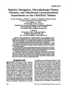
control strategies. Fig. 1 illustrates decentralized control of a distributed
computes
satellite
the satellite
relative
in the formation
decentralized,
centralized,
[Zyla
positions 93].
by
The state
or hierarchical
formation
a possible concept for using this approach to support satellite formation. In this case, each satellite independently
computes its absolute state vector using GPS and possibly "GPS-like" intersatellite measurements and transfers it via an intersatellite communications link to every other satellite in the formation. Each satellite computes its relative position to the other satellites by state uses this relative state to plan and execute formation maintenance maneuvers position
within
the formation.
control
strategies.
[Carp 00] discusses
• GPS/Intersatellite Tracking • Absolute State Vector Estimation • Absolute State Vector Differencing for Relative Navigation
a recent
investigation
Via Intersatellite Link State Vector N Via Intersatellite Link
Differencing
Configuration
with Decentralized
The absolute state vector computation can be performed method or a real-time filtered algorithm. The typical computes
the
real-time
solving a set of simultaneous of four GPS space vehicles solutions.
The
ionospheric ephemerides of the time) position
major
delays
the
of
error
Selective
on the order
filtered
Control
either an instantaneous Standard Positioning
spacecraft
position
in the
GPS
Availability
SPS
(SA)
and
measurements
corruption
point solution Service (SPS)
receiver
algorithm,
of 150 meters
arise
applied
to limit geometric solutions to approximately 100 meters when SA is enabled. Typically, GPS receiver vendors
accuracy
A real-time
three-dimensional
using GPS
Formation
time
bias
by
equations constructed using pseudorange measurements to a minimum (SVs). These products are often referred to as geometric or point
sources
and
formation
Satellite N
Satellite 1
receiver
of decentralized
• GPS/Intersatellite Tracking • Absolute State Vector Estimation • Absolute State Vector Differencing for Relative Navigation • Formation Maintenance
State Vector 1
J • Formation Maintenance
Fig. 1 State Vector
vector differencing and to maintain its desired
from
uncorrected
to the GPS
signals
and
(two-dimensional, 95 percent advertise three-dimensional
(lcr).
such as that implemented
in the GPS
Enhanced
Orbit
Determination
(GEODE) software [Godd 00], reduces the impact of the measurement errors by using an extended Kalman filter in conjunction with a high-fidelity orbital dynamics model. In addition to the simple state
vector
increasingly •
•
more
complex
approach,
the
relative
navigation
Simultaneous
estimation
measurements
between
Simultaneous
estimation
using •
differencing
GPS
measurements
Simultaneous estimation satellites and "GPS-like"
of the the local
real-time
local
filtered
can
support
the
following
approaches and
remote
and remote
of the local
approach
satellites
using
singly-differenced
GPS
SV measurement
biases
satellites
and remote
satellites
and GPS
from all satellites of the local measurements
and remote satellites using GPS measurements between the local and remote satellites 2
to all
It is anticipatedthat the more complex approacheswill provide more accuraterelative navigation solutions(for example,see[Axel 86], [Gald93], [Zyla 93], [Binn 97], [Cora98]). 3 - PERFORMANCE SIMULATION PROCEDURE The formation studied consists of four satellites maintained in eccentric Earth orbits at an inclination of 80 degrees with altitudes of approximately 500 kilometers at perigee by 7000kilometers at apogee.All satelliteshavenearly identicalsurfaceareasof 0.6613meters2 and massesof 200 kilograms.Eachsatelliteis offset from the othersatellitesby a total of approximately 10to 30 kilometers,in and/orout of the orbit plane,forming a tetrahedron.To quantify the level of absoluteand relative navigationperformancethat is achievable,GPSand"GPS-like" intersatellite measurementswere simulatedfor the two satellitesthat are in the sameorbital planeand usedto estimatetheir absoluteandrelativepositionsandvelocities. Realistic GPS pseudorangeand "GPS-like" intersatellitemeasurementswere simulated for each satellitebasedon truth ephemeridescomputedusing the GoddardTrajectoryDeterminationSystem (GTDS), which is the primary orbit determinationprogramusedfor operationalsatellite supportat GSFC. The truth ephemerideswere computedusing a high-fidelity force model that includeda 70 by 70 Joint GoddardModel (JGM)-2 for nonsphericalgravity forces,Jet Propulsion Laboratory Definitive Ephemeris200 for solar and lunar gravitational forces, a Harris-Priesteratmospheric density model, and solar radiation pressureforces. Table 1 lists the measurementsimulation options. Table 1.MeasurementSimulationParameters Parameter Measurement
.....
data rate
_Valu-e
............................
ii _ __
'_:_-_:i_ _-_-
-_i._-_i -_ ..... -
GPS: Every 1 minute from all visible GPS SVs lntersatellite: Every 3 minutes from each transmitting satellite
GPS SV ephemerides
Broadcast ephemerides
GPS signal characteristics: SA errors Transmitting antenna pattern
for July 19-22, 1998
25 meter (1-sigma) GPS L-band pattern, modeled from 0 to 90 degrees down from boresight
Transmitted power User antenna models:
28 dB-Watts in maximum gain direction
Visibility constraints
• •
Earth blockage with 50 km altitude tropospheric mask GPS SV transmitting antenna main beam and receiving antenna horizon masks
•
No constraints on intersatellite link
•
9 channels for GPS
•
3 channels for intersatellite link
•
35 dB-Herlz receiver acquisition threshold
Hemispherical
Receiver characteristics
GPS antenna: anti-nadir pointing Maximum gain : 4.9dBic Horizon mask: 85 degrees from boresight
Receiver clock bias white noise spectral density
9.616 x 10.2osecondsz per second
Receiver clock drift rate white noise spectral density Random measurement errors
1.043
Ionospheric
21.3 meters at 500 kilometer height 3.4 meters at 1000 kilometer height
The GPS
and the GPS Block
signal
I! signal
configuration strength
antenna
secondsz per seconds3
GPS pseudorange: 2 meters (1-sigma) Intersatellite pseudorange: 3 meters (1-sigma)
delays
constellation
x 10 27
was based
at the GPS receiver's
pattern
(including
on the GPS location
both the main
broadcast
was modeled
attenuation
model
that was
used
provides
realistic
for the
assuming
and side lobes).
hemispherical GPS antenna, with boresight anti-nadir pointing. threshold was set at 35 dB-hertz, consistent with the performance SV signal
messages Each
user
epoch
date
the nominal satellite
GPS
had
one
The GPS receiver's acquisition of most space receivers. The GPS
signal
acquisition
predictions
[More
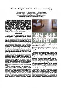
99]. The numberof simultaneousmeasurements waslimited to nine GPS(selectedbasedon highest signal-to-noiseratio) and three intersatellite,consistentwith the use of a twelve-channel GPS transreceiver.No constraintswereplacedon acquisitionof the intersatellitesignal. Fig. 2 showsthe numberof GPSSVsvisible asa function of time andaltitude.The satellites'single hemisphericalantennaconsiderablylimits GPS visibility at high altitudes.The periods of lowest visibility (4 or fewer) occur when the satellitesare at altitudesabove 5500 kilometers,where the visibility is highly dependenton the exactposition of the GPS SVs within eachorbit plane. The periodsof best visibility with 6 or morevisible GPSSVs occurwhen the satellitesarewithin the main lobe of the GPSsignal(i.e. below approximately3000kilometers). 14
12
....
-4
_10 g)
! i,
! ;
0 0.2
0.4
0.8
0.8
80OO
i-s°°°................. ?000
I-
t-I I
I
p
_,ooo -
i ....................
--
t_
I ....... I
g
30OO 2O0O
........
_ ........
1000
,--_. .......
_
V
0 0.2
0.4
0.6
0.8
Elapsed Days
Fig. 2. GPS Selective
Availability
level, using the model was used errors
when
function
(SA)
errors
were
as a Function
applied
Lear4 autoregressive integrated with a 2-meter (1-sigma) error
SA is disabled,
of the
SV Visibility
height
which
of the signal
and Altitude
measurements
at a 25-meter
(1-sigma)
moving average time series model [JSC 93]. This level to model the residual SPS ephemeris and clock
above
computed for the test orbit using the Bent noise was simulated assuming a highly-stable of 0.16(109). A twice-integrated simulate the clock bias and clock
to the GPS
is expected path
Time
by 2005. the Earth,
Ionospheric which
ionospheric model crystal oscillator
random walk model, drift noise contributions
was
delays based
were
modeled
on ionospheric
as a delays
available in GTDS. Receiver clock with a l-second root Allan variance
which is based on [Brow to the GPS measurement
97], was errors.
used
to
To minimize potentially large biases in the intersatellite measurements, each transmitting satellite would estimate its clock offset from GPS time and frequency offset from nominal based on GPS measurements and steer its clock to be synchronized to within 100 nanoseconds (30 m) with GPS time. whole
Each
transmitting
millisecond,
Alternately,
satellite
synchronized
the transmitting
part of its navigation expected intersatellite estimates were not
would
transmit
with GPS
satellite
could
a pseudorandom
Time
to within
provide
message and these biases pseudorange measurement included in the preliminary
its clock
noise
the accuracy offset
(PN)
code
of its clock
and frequency
starting offset
bias
could be included in the measurement biases in the transmitter and receiver analysis reported in this paper.
at the estimate.
estimates
as
model. The clock offset
The GPSpseudorangemeasurementsetswereprocessedusing both the point solution methodand the real-time filtered algorithm that is availablein the GEODE flight software.GEODE was also used to process measurementsets that included intersateUitemeasurements.The absolute navigationerrorswerecomputedby differencingthe truth andestimatedabsolutestatevectors.The estimatedrelative statevectorswerecomputedby differencingthe estimatedabsolutestatevectors for the two satellites.The relative navigationerrorswerecomputedby differencingthe true relative statevectorsandthe estimatedrelative statevectors. 4 - RELATIVE
NAVIGATION
PERFORMANCE
BY DIFFERENCING
POINT
SOLUTIONS This
section
method
presents
the absolute
for computation
and relative
of the
absolute
navigation
state
results
vectors.
obtained
The point
absolute position vector and receiver clock bias for each satellite which a minimum of four GPS measurements is available. This pseudorange The
measurements
left-hand
side
from
of Fig. 3 shows
errors of the point solutions The left-hand side of Fig. representative antenna, there
up to a maximum the
is five or fewer
absolute
and the geometrical
solution
provides
the
at every measurement time for method uses all available GPS
root-mean-square
(RMS)
with SA enabled. every orbit when
distribution
and
maximum
position
six or more GPS SVs are visible. position error versus time for a Using a single anti-nadir pointing fewer than four measurements are
available and point solutions cannot be computed. With or without errors of more than 1 kilometer occur for solutions near apogee, satellites
the point
method
of nine GPS SVs.
with and without SA enabled, when 4 shows the absolute point solution
set of individual point solutions are periods of about 70 minutes
using
solution
is poor.
SA enabled, where the During
the peak absolute number of visible
periods
of good
visibility
(i.e. six or more visible GPS SVs), the absolute radial, in-track, and cross-track (RIC) RMS position errors are 47 meters, 20 meters and 17 meters, respectively. Elimination of the SA-induced GPS ephemeris meters, This
and clock 5.4 meters
point
velocity
significantly
method
were
vectors,
approximately
significantly
and 4.5 meters,
solution
vectors
position
errors
10 larger
computed
meters errors
the absolute
not provide
absolute
by differentiating at
per when
RIC RMS
position
errors
to about
19
respectively.
does
computed
reduces
a
1-second
second fewer
during
velocity
a quadratic
solutions
directly.
polynomial
spacing.
This
produced
periods
with
6 or more
The
fit to the RMS
velocity
visible
GPS
absolute
four
nearest
errors SVs,
of with
than 6 GPS SVs are visible.
Absolute Position Error
Relative Position Error
700 600 500
II'-] RMS
(meters)
I
Maximum
(meters)]
400 300 200 100 0
r
>6 SVs With SA
26 SVs Without
SA
99.8% With SA
94% With SA
Percent of GPS
Fig. 3. Absolute
and Relative Satellite With Six or More
55% With SA
99.8% Without
SVs in Common
Position Errors Using Visible GPS SVs
Point
Solutions
SA
...............
250
-T-°t--al-A-bs°iu_te-P.-°-s-l-t!.°--n-En'--°r-I_ete_-
2OO o
•
:_
150
_ _
u
• •
•*
•
100 -'; .... [..o •
• ,
i
•
,
o
80
i
•
•
•
_ ;
•
Total
Relative
Position
o_
'*°
•
so ...................
I
•
i
o;
° ]
•
s :
",
"11,_
•
f'_
_
I
?.
,',
o
_
°.
,p 1.5
0.5
Elapsed
Fig 4. Absolute The right-hand
o
Satellite
for each common
solution
versus
error
navigation
error
_
time
is significantly
relative
navigation
Position
Errors
With
the relative
When
the
absolute
correlated is enabled
when
the percentage
solutions primarily
smaller
would
solutions solution
but
significant.
still
to the relative
are used
in the computation
5 - RELATIVE
equal
obtained
absolute
identical
•
..
errors
position
the
without relative error
of the absolute
NAVIGATION
errors
absolute
error.
g
e
•
2
2.5
Days
Using
obtained
GPS
Point
Solutions
by differencing
SVs is high
When
the
(99.8%
with
of common
from measurement error cancellation
would occur if the absolute point from common GPS SVs. In this of the individual
SA are differenced, position
with
the percentage
error contribution are differenced,
due to ionospheric
RMS
11;
visible GPS SVs, varying the percentage side of Fig. 4 shows the relative point
of common
the root sum square
The
.
are differenced, the solution error contributions from to SA and ionospheric delay) cancel and the relative
than
(primarily
.
1.5
SA Enabled
solution
largest relative navigation error measurement sets that are not
errors
•
1
GPS SVs used by each satellite decreases, less of the solution error is correlated. In these cases when the absolute solutions significantly less. The were computed using
.
0.5
3
satellite with six or more GPS SVs. The right-hand
the absolute errors (due
i •
0
2.5
of Fig. 3 summarizes
SA). In this case when correlated measurement
_,
Elapsed
absolute point solutions of measurements from position
"_i
**.
i
•
Days
and Relative
side
•
2
.
20 •
0
i
•
o
0
(mete_)
"
-:-v ;- "_)o:-
•
Error
t
$
• •
0o ! i
o_"_ ._ *_ .... __ : ..... •
• i
......................
RMS
error
errors)
without
(7 meters),
solutions case, the
position
cancellation
delay
SA enabled
absolute
of the
when
SA (6 meters) only
errors.
remaining
is less than
when
is
SA
is nearly
common
SVs
state vectors.
PERFORMANCE
BY DIFFERENCING
FILTERED
SOLUTIONS This section algorithm available sets,
as
GEODE in the offset
presents
well
as
processing
simulated
and relative
navigation
parameters.
sets
that
Atmospheric
included
intersatellite
pseudorange
left hand
obtained
using
a real-time
measurements.
drag and solar radiation
pressure
Table forces
measurements and clock
that were
measurement
side of Fig. 5 compares
performed. Ensemble solutions obtained by
created
by the varying
filtering
filter algorithm measurement 2 lists
were
using atmospheric drag and solar radiation pressure coefficients and 3 percent respectively from the values used in the truth
A Monte Carlo error analysis was for absolute and relative navigation
for the SA, random,
results
of the absolute state vectors. The extended Kalman flight software was used to process the GPS pseudorange
measurement
state propagation by 10 percent
generation. accumulated
The
the absolute
for computation in the GEODE
the
included that were ephemeris
error statistics were processing 50 sets of
the random
number
seeds
errors.
the steady-state
time-wise
ensemble•
true RMS
and maximum
errors of the RMS/maximum
absolute position estimates, error is the RMS/maximum
with and without SA enabled. The ensemble of the true error (difference between the estimated
true and
the true state) wise ensemble
at each time computed across all 50 Monte Carlo solutions. The steady-state timetrue RMS/maximum error is the RMS/maximum along the time axis of the ensemble
true errors,
omitting
RMS
of the absolute
error
the initial
and with SA disabled,
convergence
position
period
(l day).
and velocity
estimates
2. GEODE
Processing
Figures
6 and 7 show
for representative
with
Value
Earth Gravity model
30x30 Joint Goddard Model (JGM)-2
Solar and lunar ephemeris
Low-precision analytical ephemeris 100 meters
Initial position error in each component Initial velocity error in each component
0.1 meter per second
drag coefficient error
0.22 (10 percent)
Solar radiation pressure coefficient error Initial receiver time bias error
0.042 (3 percent) 100 meters
Initial receiver time bias rate error
1 meter per second
Estimated state
= •
GPS SV ephemerides Intersatellite transmitter ephemerides
Broadcast GPS ephemerides for July 19-22, 1998 Real-time filtered solution for same period
Ionospheric
500 kilometer minimum height of signal path
editing
Measurement
processing rate
User position and velocity GPS receiver time bias and time bias drift
GPS: All available pseudoranges
every 3 minutes
Intersatellite: All available pseudoranges
30
Absolute
SA enabled
Parameters
Parameter
Atmospheric
cases
true
respectively. Table
Nonspherical
the ensemble
Position
Error
Relative
Position
every 3 minutes
Error
25 mRMS meters) m Maximum (meters)]
2O 15 10 5 0 With
SA
Without
SA
99.8%
with
SA
94% with
SA
55% with
SA
99.8%
without
55% without
SA
SA
Percent of GPS SVs in Common
Fig. 5. Absolute
Total
and Relative Steady-State Using Filtered Solutions
RMS Position
Error
Time-Wise Ensemble True with GPS Measurements Total
(meters)
,4
__-_U_-2_-_-_I-TU_L--_TgT-T]UL----.----IT-U21T2_L'In
,_
12
....................................................
12
,o
I
Error
(millimeters
Errors
per second)
' ............ F-A-.---I.......... --i ,o
'I 6
4 t_i
RMS Velocity
Position
6
................................................
4
.,
0.5
1
1.5 Elapsed
Fig 6. Absolute
2
_Relatlvs 0.5
2.5
Error 1
,
, 1.5
Elapsed
Days
2
and Relative Ensemble True RMS Position and Velocity Errors Using Filtered Solutions with 99.8% GPS SVs in Common 7
2.5
Days
With
SA Enabled
3
Total Total RMS Position ................................... -
• 14
!
12
Absolute
Error
(mete=rs_! ............... -
Error
"
= i
14
i
12
Error
(millimeters
per second} J
'
_
RMS Velocity
.....
-
i
i
lo
i
8
8
6
6
4
4
-_i -t_" -If 0
,_ ___E.,_r-._...,'--tit
0.5
1
1.5 Elapsed
Fig 7. Absolute
With
2 2
2.5
2.5
1.5 Elapsed
Days
the absolute
filtered
point solution position errors shown meters, and 2.0 meters, respectively.
entire
1
position
errors
are
significantly
3
Days
and Relative Ensemble True RMS Position and Velocity Errors Using Filtered Solutions with 99.8% GPS SVs in Common
SA enabled,
velocity second,
O.S
3
With
smaller
SA Disabled
than
the
absolute
in Fig. 2, with RIC RMS position errors of 2.6 meters, 5.9 The filtered solutions also provide reliable, high-accuracy
estimates with RIC RMS velocity errors of 3.6 millimeters per second, 1.4 millimeters and 1.2 millimeters per second, respectively. The level of accuracy is consistent over orbit,
insensitive
SA-induced
GPS
approximately
to the number
ephemeris
2.8 meters,
and
of visible
GPS
errors
reduces
clock
4.5 meters
and
1.3 meters,
SVs at any the
specific
absolute
time.
RIC
RMS
filter
compute
the absolute
processing
was
synchronized
filter solutions
so that a high percentage
were
relative position errors of 0.17 meters, errors of 0.36 millimeter per second,
from
of the
position
errors
to
respectively.
The right hand side of Fig. 5 summarizes the relative solution errors obtained absolute filtered solutions for each satellite. The lowest relative errors were absolute
Elimination
per the
common
of the measurements
SVs (99.8%
0.56 meters, and 0.17 meters, 0.09 millimeter per second,
by differencing obtained when
with SA),
yielding
the the
used RMS
to
RIC
and RMS RIC relative velocity and 0.I millimeter per second,
respectively. Fig. 6 also shows the relative ensemble true RMS position and velocity errors versus time when the percentage of common GPS SVs is high (99.8% with SA). In this case, when the absolute solutions are differenced, the error contributions from correlated measurement and dynamic errors cancel and the relative navigation errors. Since the satellites are in nearly the same and
a large
percentage
of the
dynamic
error
accuracy is significantly better than the absolute orbits, the dynamic errors are highly correlated,
contribution
cancels
in all of these
cases.
When
the
percentage of common GPS SVs used by each satellite decreases, less of the measurement error is correlated. Consequently, the absolute error cancellation in the differenced solutions is less and relative errors increase as the percentage of common GPS SVs decreases. With SA disabled (99.8% without
SA),
complete
the RMS
satellite
A preliminary measurements state vector pseudorange
relative
synchronization
position
errors
(99.8%
are comparable
to the
SA-enabled
from the other
with
nearly
with SA).
assessment was made of the impact of augmenting with "GPS-like" intersatellite measurements. In the approach of the local satellite was estimated independently using measurements
case
satellites
in the formation.
the GPS evaluated, GPS and
This simulation
pseudorange the absolute intersatellite assumed
that
a navigation message containing the absolute state vector of each of the transmitting satellites would be provided to the receiving satellite using the intersatellite communications link and used to model the intersatellite measurements and to compute the relative state vector by the state vector differencing by estimation absolute and measurements.
method.
When
the ephemeris
provided
using only GPS measurements relative solution errors are When
the
true
ephemeris
for each transmitting
(with RMS comparable
of each
transmitting
satellite
was
that obtained
position errors of about 8 meters), the to those obtained using only GPS satellite
was
provided,
the
absolute
solutionerror for the local receivingsatellitedecreased to below2 metersbut the relative navigation increaseddueto the reductionin the cancellationof the solutionerror contributionsfrom correlated dynamic and measurementerrors. Thesepreliminary results indicate that high accuracyrelative navigation solutions using cross-link measurements will requirethat cross-link measurementsbe includedin the solutionsfor all the satellitesin formation, in orderto maximizethe cancellationof the absoluteerrorcontributions. 6 - CONCLUSIONS AND FUTURE DIRECTIONS This study assesses the feasibility of using statevector differencingfor relative navigation.When SA is enabled,relativenavigationaccuraciesof betterthan 10metersRMS areachievablewhen six or more GPSSVs aremutually visible by differencingpoint solutions,if only measurementsfrom GPS SVs commonto both satellitesare usedin the absolutesolutions.However, the use of point solutionsis not suitablefor continuousreal-timenavigationin configurationswhere fewer than six GPS SVs are visible during significant portions of the orbit. For the 500 by 7000 kilometer formationusedin this study,reliable pointsolutionswould beavailableonly about50 percentof the time using a single hemisphericalantenna,improving to about90 percentof the time using an omnidirectional antennaconfiguration.Becausepoint solutions do not provide accuratevelocity estimates,they arenot suitablefor applicationsin which statevector informationmust be predicted aheadin time, e.g.,to supportautonomousmaneuverplanning. If the absolutestate vectors are computedusing a high-accuracyfilter, the relative navigation accuracyimprovesto betterthan 1 meterand0.5 millimeter per secondRMS if only measurements from GPS SVs common-to both satellites are used in the absolute solutions. This level of performanceis maintainedover the entireorbit, insensitiveto the numberof visible GPSSVs at any specific time. This relative accuracy satisfies the most stringent navigation requirementsfor autonomousmaneuverplanning of the formation studied.The relative accuracydegradesas the percentageof measurementsfrom commonGPSSVsthatareusedin the point solutionsdecreases. In formationsfor which the separationdistancesarelessthan 100kilometers,suchasthe formation studied in this report, GPSSV visibility will be nearly identicalfor all usersatellites.In this case, restrictingthe measurements processedto thosefrom commonGPSSVs is not unreasonable. Future directions will initially focus on a detailedinvestigation of improvementsto be realized throughthe simultaneousestimationof the local andremotesatellitestatevectors.Expectationsare that the relative navigation performancewill be improved through the processingof singledifferenced measurementsor the estimation of GPS-SV-relatedbiases and the processing of intersatellitemeasurements to simultaneouslyestimatethe locationof all satellitesin the formation. The GEODE flight software, which has recently been enhancedto support multiple satellite estimationandadditionalmeasurement types, will be used in these studies. The relative navigation version of GEODE is being integrated GSFC GNCC. This formation-flying in GNCC's
formation-flying
into a low cost GPS satellite receiver receiver will be used to demonstrate
being developed by the end-to-end performance
test bed.
REFERENCES [Axel
86]
P. Axelrad and J. Kelley, "Near using GPS," Proceedings of Conference,
[Baue
99]
F. Bauer Enhanced
November
Earth Orbit Determination the 1986 1EEE Position
Navigation Navigation
1986, pp. 184-191.
et al., "Enabling Spacecraft Autonomy Technology,"
September
and Rendezvous Location and
Formation Proceedings
Flying Through Spacebourne GPS and of the ION GPS-99, Nashville, TN,
1999
[Binn
97]
P. Binning, Proceedings
"Satellite to Satellite Relative Navigation of the 1997 ION National Technical Meeting,
[Braz
96]
J. Brazzel, et al. "Flight Test Results from STS-69," Space Flight Mechanics 1996, AAS 9
Real-Time Publications
Using January Relative Office,
GPS Pseudoranges," 1997, pp.407-415. GPS Experiment San Diego, CA
on
¢
1
[Brow
97]
R. G. Brown Filtering,
[Carp
00]
J. R.
and P. Y. C. Hwang,
Third
Carpenter,
Formations,"
[Gald
98]
93]
"A
March
T. Corrazini,
John Wiley
264
20-22,
et al.,
at
Signals
and Applied
Kalman
1997
Invetigation
presented
of Decentralized
the
IEEE
Control
Aerospace
for
Satellite
Conference,
Big
Sky
2000
"Experimental
Formation
Flying
Spacecraft,"
J. Galdos,
et al.,
"A GPS
Capture,"
to Random
and Sons,
Preliminary
Paper
Montana, [Cora
Edition,
Intro_htction
Proceedings
Demonstration
Navigation, Relative
of the
of GPS
45(3),
ION
Sensor
for
pp. 195-207.
Navigation
1993
as a Relative
Filter
National
for Automatic
Technical
Rendezvous
Meeting,
and
January
1993,
pp.83-94. [Godd
00]
Goddard
Space Enhanced
Version
5, T. Lee
February [Gram
94]
C.
J.
[Kama
[More
99]
98]
the
99]
Global
Space Charles
Kamano,
Flight
et
al.
1999
Moreau
Moreau
and
Space [Zyla
93]
H.
et
al.,
GPS
Flight
System
Specifications,
Sciences
Corporation,
L. Zyla Vehicle
"GPS
Evaluation
Receiver
1998,
of
Autonomous AIAA
of STS-80
AAS Publications
and M. Montez, "Use of Two Orbital Rendezvous," Proceedings
301-312
10
Filters,
William
Docking
Conference,
Portland,
Analysis
Nashville, and
Eccentric
Relative
Mechanics
Rendezvous
GN&C
Post-flight
Massachusetts,
Flight
Spacecraft
19-2 l, 1997, pp. 123-133
GPS Navigation
Architecture
in Highly
Theory
1994, pp.253-267
of the
May
for
Flight
1993
of the 1999 "RGPS
17-19,
of the SSTI/Lewis
3345,
of the ION GPS-98,
Cambridge
et al. "Results
June
(TONS)
MechanicsEstimation May
Proceedings
Bias Models
Proceedings
System
Navigation
(GPS),
Laboratory,
Marcille,
Flight 3265,
Publication
Range
Navigation
Mechanics
of the
System
Conference
and
Navigation
Publication
"Autonomous
Proceedings
ION Meeting,
E. Schiesser,
Proceedings
"Result
OR, August
Autonomous
98]
Positioning
Mathematical
by Computer
Onboard
Conference
Draper
of ETS-VII,"
M.
prepared
"TDRSS
Center,
Stark
Experiment G.
Global
(GEODE)
(CSC),
Positioning
1997, NASA
M. Lear,
Annual [Schi
al.,
and T. Lee,
Demonstrations," [More
A. Long
NASA
A. Long,
Johnson
I.
CSC-96-968-01ROUD1,
Determination
Experiment,"
Symposium [JSC 93]
et
1994,
R. Hart, Using
and
Gramling
Symposium 97]
Center,
Orbit
2000
Qualification
[Hart
Flight
(GPS)
Expected
Orbits,"
June 28-30, GPS Office,
of
ARP-K
TN, September
Flight 1998
Performance
Proceedings
of the
for 55th
1999
Navigation San Diego,
Flight
Experiment,"
CA
GPS Receivers in Order to Perform Space of the ION-GPS-93, September 1993, pp.