Autonomous Satellite Formation Assembly and Reconfiguration with Gravity Fields 1 Ella Atkins
[email protected]
Yannick Penneçot
[email protected]
University of Maryland Space Systems Laboratory Neutral Buoyancy Research Facility, Building 382 College Park, MD 20742 Abstract— Spacecraft formation flight may increase data coverage area and accuracy for a myriad of space-based experiments. To prevent ground operations support from scaling with number of satellites, we propose a control architecture that describes a formation as a virtual body, such that the operator controls the group as if it were a single entity. We overview the components of a satellite formation flying architecture then outline a constrained multi-agent planning approach to decompose the specified formation geometry into an optimized set of synchronized satellite waypoint sequences. To illustrate our approach, we describe a two-satellite planar Earth-orbiting formation for far-field interferometry and show results from path optimization for circular and elliptical orbits.
collection areas larger than existing ground-based observatories. Astronomy -based formation flight missions have been proposed to perform black hole spectral analysis, gravitational waves detection, and extrasolar planetary observation. In addition to far-field observations, we can gain significant understanding of our own planet by pointing the formation sensors inward from low-Earth orbits(LEO). With such formations, meteorologists and climatologists will greatly enhance their understanding of atmospheric patterns through long-term observations of atmospheric phenomena impossible to continuously monitor with existing single-satellite data collection platforms.
TABLE OF CONTENTS 1. 2. 3. 4. 5. 6. 7.
INTRODUCTION BACKGROUND FORMATION SPECIFICATION TRAJECTORY PLANNING A STRODYNAMICS "PLANNING EXPERTS" CASE STUDY: 2-SATELLITE INERTIAL FORMATION SUMMARY AND FUTURE W ORK
1. INTRODUCTION In recent years, spacecraft formation flying has become a topic of increasing interest for both the astronomy and Earth science communities. Spacecraft volume and mass pose hard constraints, so by necessity onboard instrumentation possesses limited capabilities. A proposed solution to enhance coverage area and data resolution is to utilize several coordinated spacecraft as a "virtual" science platform, providing capability analogous to ground-based systems such as the radio telescope very large array (VLA). Several science mission types can benefit from this new approach to formation-based data collection. A coordinated array of astronomical observation spacecraft can observe targets without the distortion of Earth's atmosphere but also with the advantage of apparent 1
0-7803-7231-X/01/$10.00/© 2002 IEEE, Paper #296
To be specific, we define the term formation flight to reference a group of satellites or spacecraft whose relative state (position and motion) is constrained to meet mission goals. In the general case, we define two formation classes, the Virtual Rigid Body (VRB) and the Virtual Flexible Body (VFB) [9] configurations. As their names suggest, the former will require fixed relative position between each satellite and an overall formation reference coordinate frame, while the latter will permit the specification of relative motion between satellites and the overall formation "body". Maintaining a formation may require some vehicles to follow non-Keplerian [artificial] orbits. This type of motion can only be achieved by active control to counter gravitational field forces. Moreover, for some applications, extremely high accuracy for all six translational and rotational degrees of freedom (DOF) is required. We are working as part of a research team to define an overall architecture that allows accurate formation specification and control from mission operator all the way down through 6-DOF spacecraft controller and state estimator. For some missions, the distance between satellites may be relatively small, especially during transition between virtual body shapes. To decompose a specified formation geometry and task set
into a waypoint-based path, we require several capabilities. First, if not pre-determined by uniqueness of spacecraft instrumentation, we must match individual satellites with elements in the VRB/VFB. Next, we must compute waypoint paths to both assemble and maintain our formation in the presence of gravitational fields. Throughout, we must verify that satellite paths satisfy problem constraints, including fuel usage and minimum separation (for closely-spaced formations). The overall problem of automated formation management is quite extensive, so we have narrowed our research focus to the orbit/path planning problem. Our planner contains a search engine coupled with specialized astrodynamics algorithms as "planning experts" to optimize both overall formation and individual spacecraft trajectories so that they minimize fuel consumption. This formation planner considers two distinct scenarios: assembly and maintenance. For assembly, the user defines satellite initial states (e.g. after launch vehicle release), maximum formation assembly time, and final formation shape (e.g. VRB "nodes"). To situate the formation in space, the user specifies a formation "centroid" frame V with respect to an orbiting or fixed target coordinate frame T. Maintenance consists of satisfying long-term spatial and temporal formation constraints. For a VRB, a controller must accurately maintain a fixed shape, while for a VFB, a trajectory mu st meets mission goals while satellites move in a prescribed fashion with respect to their centroid. We begin this paper with a brief overview of existing practice for satellite operations. We define our formation flying architecture as well as the [limited] set of astrodynamics algorithms used to minimize overall fuel cost over each observation. Finally, we present examples of an Earth-orbiting formation where the two component satellites act as an interferometer to observe a distant astronomical object.
2. BACKGROUND Most active satellites require a minimum of one ground support staff to compute orbit corrections, monitor onboard anomalies/faults, and monitor onboard data collection as well as the critical communications link. Researchers are progressing toward an "on-call" response strategy for repetitive operations [4] but still require experts whenever orbit adjustments must be executed. To conserve fuel, most satellite operations are conducted from natural (drift) orbits with onboard attitude (pointing) control supplemented by occasional orbit disturbance corrections dictated by ground personnel. When a satellite must shift to a new orbit, the operator must compute an efficient and accurate burn sequence, which is tested in simulation then finally transmitted to the satellite. This manual orbit calculation and simulation process is time-consuming for one satellite and prohibitively support-intensive for a large satellite group.
Formation flight introduces another challenge with relative position constraints. To-date, research has emphasized GPS and laser-based sensing techniques with an ambitious goal of picometer accuracy. It will be essential to support such sensing technology with actuators and an active closed-loop position control strategy that can handle this accuracy requirement. With the "continuous thrust" paradigm shift arises new challenges in the form of fuel management, since even small corrections executed over a long observation time period may exhaust fuel supplies with surprising speed. The tradeoff between accurate control and fuel conservation suggests careful specification of conditions under which active control versus drift will best serve long-term mission goals. NASA has begun a series of flight experiments with a simple chaser-follower formation (EO-1) in which all satellite orbits are "natural", meaning that active control is required only to counter perturbations rather than "fight" gravitational forces. This experiment has been designed and will be controlled manually. ESA is also working on a project of satellite formation XEUS. This project consists of a large space telescope with a focal length so large (50 meters) that it is not realistic to have both elements rigidly attached.
3. FORMATION SPECIFICATION Our goal is to enable a satellite formation to be assembled and maintained given arbitrary initial states and formation geometrical and orbital constraints. We assume the user defines the mission, then the system optimizes trajectories for all formation satellites. To prevent scaling difficulties as formation group size increases, we provide an interface that allows the user to specify high-level formation parameters then employ automatic planning and trajectory generation techniques to develop efficient paths for each satellite. Formation parameters include geometry, orbital constraints, and attitude, supplemented by individual satellite attitude and relative motion as necessary. Waypoint selection minimizes fuel expenditure subject to synchronized timing constraints for the satellites. As shown in Figure 1, computation of the waypoint trajectories is ground-based to facilitate high-speed processing and adjustable planner autonomy levels from manual to fully-automated. Once desired waypoint trajectories have been computed in terms of coordinate frames and waypoint sequences (plans), they are transmitted to each satellite. Onboard each [simulated] satellite, waypoints are interpolated to yield individual satellite trajectories. The 6-DOF controller calculates the thrust levels, and the simulator outputs resulting satellite trajectories using a high-fidelity dynamic model. See [10] for more details on the formation flying architecture and its implementation.
STK™ 3-D VO
GUI Mission Parameters
Waypoint Planner
Frames Plans
Trajectory Synthesis
Control Laws
Thrust Levels
Satellite Dynamics State
State
Satellite-1 Ground station
Trajectory Synthesis
Control Laws
Thrust Levels
Satellite Dynamics State
State
Satellite-n
Figure 1 - Formation Flying Control Architecture To precisely specify coordinated geometry and motion of multiple bodies in 3-D space, we define a set of coordinate frames and a waypoint plan specification language. For any formation, we first define a "target" coordinate frame T to be tracked by the entire formation. T frame orbital parameters specify its translational motion, while attitude is defined with respect to either inertial or LVLH (Earth-pointing) coordinates. The actual position of the overall formation is frame V, defined relative to the T frame. Generally, these frames will be aligned when considering a single formation flight mission. However, the separation of V and T frames allows our system to represent multi-body tracking operations such as rendezvous and docking. We define a set of coordinate frames Dk that specify individual satellite positions and attitudes relative to the V frame. Figure 2 illustrates the frame attachments we have defined for formation flight. T-frame D1 frame
D3 frame
V- frame I-frame
D2 frame
Figure 2 - Formation Frame Attachment In the simplest case, a formation specifies a virtual rigid body (VRB) [9] in which the overall formation body may
translate but individual elements maintain a fixed position and attitude with respect to each other. This case would be utilized by astronomical missions in which multiple satellites are used to form a "very large array" in space. For a true VRB, the Dk are constant, being used only to define the static formation shape. In this case, individual satellite trajectories are fully specified by rigid transformations from a single V frame motion sequence. A direct extension of the VRB is a pseudo-VRB in which formation shape is rigid but individual satellite attitudes vary. A pseudo-VRB is illustrated by a telescope mirror, in which individual segments can be "tuned" to focus the image. The translational component of an associated waypoint plan is still fully specified by a V frame motion sequence. However, for each satellite k that rotates relative to V, an additional 3-DOF attitude waypointbased motion sequence for Dk must be specified. The most general and complex class of formation we represent is a virtual flexible body (VFB), in which the overall formation may change shape and orientation, enabling arbitrary individual satellite (Dk ) and formation (V) motion to be represented. Waypoint plans require 6-DOF V frame and Dk frame motion sequences. The VFB allows localized satellite motion within the formation to broaden data collection area or improve accuracy. In the limiting flexible case that assumes a liberal definition for the term "formation", V and T frames are aligned, while individual satellites follow arbitrary waypoint paths relative to V. This strategy may be used to define any combination of satellite orbital motions and may simply be used to synchronize satellite activities (e.g., orbital periods) without also subjecting these satellites to relative geometric constraints.
In order to specify the formation, the user provides: • The T frame definition, including its [natural] orbital parameters and its attitude. Attitude may reference either the central body or an inertial frame. • The position and orientation of the V frame relative to the T frame. The orientation of the V frame can be constant or a function of time/orbital position. • The location of the Dk frames in the V frame. This set of frames specifies the geometry of the formation as it is going around the central body. Dk frames are typically specified with respect to the V frame. For example, given a two-satellite formation pointing at a distant galaxy, the attitude/pointing of the T frame will be inertial. The V frame will be fixed in the T frame (and may match T precisely for simplicity). The two Dk frames will be positioned so that satellites are at the appropriate distance from each other, with attitude matching the V and T frames to collect data from the observation target.
4. TRAJECTORY PLANNING From a planning perspective, the simplest strategy for formation flight is to assemble the desired geometric configuration and continuously maintain this shape until commanded to alter the formation. For a VRB in flat space (i.e., no gravitational effects), this approach is intuitive and effective. This method also succeeds in gravitational fields provided the formation may be formed from "natural" or near-natural orbits (e.g., chaser-follower formations such as the EO-1 mission). However, arbitrary formation geometries, most easily visualized for the VRB, will require fuel expenditure both to assemble and maintain the formation. Because onboard satellite fuel is limited and costly, we must trade off formation assembly and maintenance time with fuel expenditure. To-date, this tradeoff has led to the manual computation of clever orbital designs with near-natural orbits that automatically assemble the satellite formation for limited time per elliptical orbit (e.g., near apogee and/or perigee). We wish to capture this design technique in our path planner, such that it can perform the search for a valid set of satellite trajectories based on a cost function to trade off mission data collection constraints with expected fuel utilization. From the fuel perspective, each satellite should have a natural orbit, while accurate formation maintenance in the general case will require substantial fuel expenditure to counter gravitational effects (and/or acceleration). Our architecture supports three types of control modes: drift, impulsive (∆v) thrust, and 6-DOF active (controlled) trajectory following. During drift, no actuation forces are applied to the spacecraft. Impulse maneuvers are computed by the path planner and assumed instantaneous for our analysis to-date. When entering a data acquisition pass, the impulse is used to match formation (V frame) velocity for a VRB or individual Dk frame velocities for a VFB. When entering a drift orbit, an
impulse is used to set spacecraft velocity so that a = natural orbit brings all formation satellites to their next observation stations synchronously. The job of the path planner is to define the space of possible observation segments that meet mission constraints and use drift orbits to connect these observation segments in a fuelminimizing fashion. Three-dimensional multi-agent path planning techniques range from A* or dynamic programming [11] in which space is discretized to cost-based optimization [4] for boundary-value problems. These techniques may be straightforwardly mapped to satellite formation flying under the assumption that gravitational field effects are not significant. As an example, consider formation assembly for n-satellites. A centralized search engine matches satellites to goal locations based on travel distance and collision avoidance. The planner search space is defined by the combinatorial mappings from satellite initial states to goal locations, while constraints are based on fuel limitations, reconfiguration time, and collisions. In curved space, traditional path planning assumptions may not apply. For example, distance from initial to goal position cannot approximate either fuel cost or travel time. We have coupled a discrete-space path planner with astrodynamics "planning experts" (e.g. Lambert algorithm [3]) to both match satellites to waypoints and build efficient paths through gravitational fields to reach these waypoints. The cost for one satellite to reach the goal is no longer the distance between two locations. Instead, cost is a complex function of the initial and goal orbits, as well as the time to transfer for formation synchronization purposes. Search-space complexity also increases, as illustrated by the command "move to orbit X", which incurs fuel costs based both on variations of the six orbital elements and also formation synchronization constraints given that goal states are non-stationary. For this initial research, we have implemented a bruteforce (uninformed [11]) search strategy to identify optimal orbits. The user manually specifies formation parameters as illustrated below in Section 7, then the search engine exhaustively searches through the parameter space for the set that minimizes the userdefined cost function, typically dominated by spacecraft fuel usage. Below, we describe the simple set of "planning experts" utilized by the planner and describe results from a 2-satellite interferometry "case study" that illustrate the optimization process.
5. ASTRODYNAMICS "PLANNING EXPERTS" The ultimate set of "planning experts" could compute optimal trajectories given arbitrary gravity fields for any set of satellite initial states, final states, and transfer times. However, such calculations in the general case are computationally complex, and numerical solutions
methods do not always guarantee an optimal result. We opted to build our initial astrodynamics library from optimal techniques at the cost of limiting the set of orbits that could be modeled. Specifically, we have employed the Lambert's solution method [2], capable of computing optimal transfers between in-plane orbits, as our sole planning expert. This method provides a basis for formation optimization in a variety of cases and can be supplemented in future work by other experts that would accommodate perturbation models or even multi-body problems (around Lagrange points for example). Ideally, all satellites in a formation could be maintained in natural, approximately Keplerian, orbits. Such formations require zero fuel to maintain except for disturbance rejection. This approach is possible when a formation admits zero-fuel design, such as for a chaser-follower configuration, a formation near a Lagrange point, or a formation such as LISA where the orbits have been cleverly chosen in three-dimensional space so that the distance between the satellites is constant and the plane of the formation always points at the central body (i.e. the Sun). For cases where natural orbits cannot satisfy mission objectives, the job of the planner is to select orbital parameters for each satellite that minimize the overall fuel required.
expert[3][2].2 This function examines the transfer between two position vectors. It uses the “Lambert theorem” that states: "the orbital transfer time to traverse an elliptic arc depends only upon the semi -major axis, the sum of the distances of the initial and final points of the arc from the center of force, and the length of the chord joining these points." Our function takes the two radii vectors that start and finish the elliptic arc and the time of transfer as input and outputs the required speed vector at the beginning and the end of the elliptical arc. Several different algorithms exist to solve this problem. We chose the strategy described by Battin [3] because this routine does not suffer from the 180º-degree transfer difficulty plagued by other Lambert’s routine implementations [11] Distant Object
Yi Controlled Segment
?
ω
Maintaining a satellite on a non-Keplerian orbit can be tremendously expensive in fuel over time. Moreover, the observation target may be occluded by earth for some period of time. There is no need to actively control the formation during this period. Additionally, as we later demonstrate, careful selection of orbit segment (e.g. near apogee) may significantly reduce fuel required for satellites to maintain non-Keplerian formation geometries for extended time periods. Our VRB representation includes a hybrid orbit configuration where only part of the orbit is actively controlled while satellites drift during the rest of the orbit. Consider the limiting cases. If active control occurs throughout the orbit, the formation VRB will be maintained continuously but at potentially high fuel cost. If only natural orbits are used, then arbitrary formations will assemble only periodically (e.g., at apogee) and even then for brief time periods. Allowing alternate periods of drift-active control allows us to conserve fuel but also achieve non-Keplerian formations for data acquisition. Consider the case in which we allow one control and one drift segment per orbit. Because formations are periodic, the members of the formation exit drift mode precisely where active control (thus data acquisition) begins. In this case, the spacecraft must leave the controlled portion of their orbit coordinated in time and in space with the other members of the formation at the end of the drift. This coordination is achieved by giving the satellites an impulse in the direction computed by the Lambert
Reference Orbit
θ ?
Figure 3 - Search space parameters for an elliptical formation. To capture VRB constraints, the formation must maintain the desired shape (i.e. position of the Dk frames in the V frame), in the desired pointing orientation, within defined orbital altitude constraints and for sufficient data collection time. We are then free to search through orbital parameters (shown in Figure 3) to select activelycontrolled orbit regions and the specific T frame definition that minimizes fuel expenditure and maximizes observation time. For generalized planar formations, we define the search parameters as follows: λ, the portion of the orbit where the formation is actively maintained, where 0< λ =360. If λ is 0 then the satellites will be aligned for an instantaneous time (e.g., at apogee), and there is no actively controlled mode. If λ is 360 degrees, the formation is controlled during the entire orbit, so no hybrid orbit solution is required.
2
We ignore burn time and reorientation maneuvers required to apply main engine impulsive thrust. Such costs will be incorporated in future work.
Xi
?, the angle from the semi-major orbit axis to the center of the controlled orbit segment, as shown in Figure 3. This angle fixes the position of the controlled portion of the formation. When ? is 0, the controlled portion centers on perigee, or when ? is 180, the controlled portion centers on apogee. d, the offset of the V-frame with respect to the T frame in the direction of the two farthest satellites. This parameter is 0 when V and T are aligned. Although we consider radial distance only in this initial work, d will generally be a three-dimensional vector offset. tdrift , the time during which the formation drifts per orbit. The formation begins drift with an impulse (for each satellite) to achieve synchronized Lambert's solution orbit segments when the origin of the V frame reaches the end of active control region λ. After tdrift , a final impulse is applied to each satellite to reassemble the formation for the next control period. Note that tdrift will generally not match the time associated with the equivalent T frame drift orbit segment, since we adopt the tdrift that minimizes fuel expended by all satellites for the initial and final impulse maneuvers. Once we find the optimal parameter set (λ, ξ, d, tdrift ), the required trajectory for each satellite can easily be found. In the controlled portion, each Dk frame position is found by a rigid coordinate transformation from the T and then V frames. For the drift portion, we know the orbit of each satellite from the Lambert expert; the trajectory can then be computed from the defined orbital elements. As discussed previously, this trajectory is downloaded to the controller as a waypoint sequence that includes mode (e.g., active, impulse, drift), velocity, angular velocity (in general), and time. Generally, spacecraft will utilize different thruster types for impulsive versus continuous thrust. High thrust engines used to achieve impulsive maneuvers typically have low specific impulse (Isp ), while high Isp , low thrust engines may be utilized for continuous active control. thruster for active control since there is no need to apply a great force on the satellite for active control, but the force has to be applied for a relatively long period of time. For this research, our impulsive thrust magnitudes are relatively low, and we presume the use of the same Isp for all maneuvers when converting from required ∆v to mass. These results can trivially be recomputed given a different specific impulse set.
6.
2-SATELLITE INERTIAL FORMATION
To ground our discussion, we analyzed a planar formation with two satellites. We defined this formation on an equatorial orbit to avoid Earth oblateness effects. This formation is the first step to analysis of larger-scale formations; its simplicity enables intuitive understanding of the impact of each variable (λ, ξ, tdiff, d) on path cost.
This understanding will assist our exploitation of symmetries and orbital phenomena (e.g., apogee corrections require less fuel than their perigee equivalents) for more complex formations with n satellites. Both circular and elliptical orbits have been simulated in this study. Our goal is to demonstrate the complete planning process from defining the formation and optimality criteria to identifying the globally-optimal solution via exhaustive parameter search. Since our VRB architecture strives to minimize the work of the ground controller, we intentionally minimize the number of parameters the user must specify. In our system, the user first specifies orbital elements of the Tframe (a T, eT, ωT). The user also specifies the position of the Dk frames relative to the V frame, which translates to distance between satellites in our two-satellite interferometry example. Formation geometric parameters yield tradeoffs between scientific yield and fuel expenditure. For example, increased separation distance improves measurement accuracy for sensors such as an interferometer. Decreased separations in arbitrary formations also tend to decrease fuel required for formation maintenance, with the limit (d=0) permitting a point formation that follows the T frame naturally. We require the user to specify precise geometry currently, but in future work, we will allow the user to specify a range of viable values and optimize fuel costs over that range. The four parameters described above (λ, ξ, d, tdrift ) form the search space of this case study. Parameters λ and ξ have full range from 0 to 360 degrees. Currently, the user defines d explicitly, and our Lambert's solution module searches tdrift to find the optimal value. The granularity of the grid is constant for each parameter. Angular resolution is tenths of radians, and the time is divided into tenth of seconds for geo-stationary orbits. The offset of the V frame from T is examined every 100 m (ranging from sat-1 aligned with T to satellite-2 aligned with T) to determine optimal placement of the satellite pair relative to the reference orbit. As seen in Figure 4, the total quantity of fuel expended in both satellites for continuous thrust depends very little on V frame offset so long as it stays within boundaries (i.e. , Dk frames on either side of the T frame). Of course, the further a satellite from its natural orbit, the more fuel it will require to follow its non-Keplerian trajectory. This parameter is extremely important both to minimize overall fuel use and to equalize the amount of fuel in the satellites relative to each other.
orbits. To illustrate these approximate calculations, we apply Newton’s 2nd law. Applied forces include gravitational attraction by the central body and the force induced by spacecraft thrusters. To maintain VRB shape, each satellite must follow exactly the same trajectory as the T frame with constant offset given by Dk. This implies that the acceleration of the satellite is the same as the acceleration of the T frame. We can compute the value of T frame acceleration by observing that the naturallyorbiting T frame has balanced centripetal acceleration and gravitational forces. The thruster force for any satellite is then given by Equation (1):
Ft =
Figure 4 - Fuel expended during continuous thrust as T frame offset varies relative to each satellite.
µ .m µ .m − 2 2 ( Rref + ∆r) Rref
(1)
where ∆ r is the difference between the altitude of the satellite and the altitude of the T frame, Rref is the altitude of the T frame with respect to the center of the attracting force, and m is the mass of the satellite (see Figure 7). Assuming Rref>>∆r, this expression can be simplified to Equation (2):
Ft ≈− m sat1+sat2
1+
µ Rref
(2)
2 .∆r ∆r
sat1
sat2
Distant Object
Rref
Figure 5 - Mass of fuel expended for impulsive thrust as a function of tdrift , all the other variables fixed Figure 5 illustrates the dependence between drift time and impulsive thrust fuel required for each satellite's associated Lambert's solution. Note that the x-axis is offset by the time required for a satellite to drift on target orbit T for orbit interval (360 – λ). As shown in Figure 5, there exists a region where the total fuel cost (sat1+sat2) varies minimally for both satellites. We can select any near-minimum point in this valley to equalize the fuel quantity in the formation satellites without altering the fuel expended during active control mode. In the following paragraphs, we study independently the cost in active control mode and the cost of the ∆V. Then, we combine the two to find a globally-optimal solution over the entire orbit. First we compute the continuous thrust cost. From basic orbital mechanics, we can intuitively discern that minimum fuel will be expended for a satellite if the Dk frame is very close to the T frame. Moreover, one can hypothesize that formations far from the central body will be less expensive than low-altitude
R1 R2
Rref
*NOT TO SCALE
Figure 6 - Different parameters involved in the amount of fuel needed for the continuous thrust Equation (2) verifies our assumptions. Formations far from Earth (i.e., large Rref) will require less thruster force (Ft ) than those close to Earth, and satellites close to the T frame in altitude (i.e., small ∆r) will require less force (fuel) than those far from T. This simplified analysis indicates that two primary parameters will determine the amount of fuel to be spent for the continuous thrust: Rref, and ∆r. The following describes how these crucial values vary with other parameters.
Consider orbit eccentricity (e) and its effects on fuel cost (or equivalently thruster force to maintain the formation). When e=0 (i.e., T frame is on a circular orbit), Rref is constant throughout the orbit, and ∆r is minimum when the formation is on the line from the earth to the distant object, as shown in Figure 7. When e > 0 (the T-frame is on an elliptical orbit), Rref is no longer constant, varying from a minimum at perigee to a maximum at apogee. A high orbital altitude minimizes fuel, so if the semimajor axis is aligned with the distant object (for interferometry), the ξ for a given λ that minimizes overall fuel utilization is at apogee (ξ=180 degrees). If the vector d connecting the two satellites is along any other direction, then the problem is not so trivial. For an object 90 degrees from the semi-major axis, for example, Rref will be maximum at apogee, but then ∆r will be minimum, so the optimal solution ξ may reside in an intermediate location.
entire orbit is actively controlled, so the cost is no longer dependent on ξ. Figure 9 shows an analogous plot but with e=0.5. For this plot the observed object is aligned with the eccentricity vector (semi-major axis). So, as predicted, the minimum occurs when ξ=180 degrees (apogee), where Rref is maximum and ∆r is minimum. At perigee (ξ=0), the satellite is as close as possible to the earth. Since Rref is small the fuel required grows dramatically as one approaches perigee. However, ∆r is also small at perigee, thus it produces a local minimum. Note that Rref (50000 km for this example) dominates the fuel effects given the relatively small value of ∆r (10 km). As λ increases, the plot is flattened since more of the orbit is actively controlled. For λ=360, the plot will be completely flat as a function of ξ, since formation is maintained throughout the orbit.
B
ξ A
A
B
Figure 7 – Variation of Rref, and ∆r, along a circular orbit Now consider the parameter λ. It is evident that the longer the formation is maintained, the more fuel will be expended. However, long-duration observations may be desirable for many scientific missions. In Figure 8, we plot the amount of fuel required for active control mode of both satellites divided by the time during which the formation is maintained as a function of ξ, and λ. In this figure we see fuel cost (expressed in fuel mass per second of observation time) results for a circular orbit. When λ is small, we obtain the anticipated result; fuel expended per second of observation is maximum when the formation is centered at 90 and 270 degrees, corresponding to the case for maximum overall ∆r. The minima are also as expected (ξ at 0 and 180) because the satellites are close to their Keplerian altitude. For values of λ above 180 degrees, the minima and maxima are inverted. This condition is illustrated by the former minimum case of ξ=180. With λ>180, the only region where the formation is not actively controlled is near the zero-degree area, which represents the other minimum fuel orbital segment. For λ=360, the
Figure 8 - Continuous thrust fuel mass per second of observation (e=0, ω=0, θ=0).
Figure 9 - Continuous thrust fuel mass per sec of observation (e=0.5, ω=0, θ=0)
Figure 10 shows fuel required per second of observation given a target oriented in a direction perpendicular to the eccentricity vector (θ=90 degrees). The maximum amount of fuel required is at perigee, since the satellites are both close to Earth and have maximum ∆r. In this case, the minimum is at ξ=180 for any value of λ, illustrating the dominance of changes in Rref over our small ∆r for highlyelliptical orbits.
trailing satellite assumes a lower (faster) orbit. In the second case (ξ=90 degrees) minimum fuel is required for λ=180 degrees because the satellites more naturally drift synchronously to their respective final altitudes 180 degrees later.
Figure 11 - Mass of fuel for the impulse both at the beginning and the end of the drift mode (e=0, ω=0, θ=0) Figure 10 - Continuous thrust fuel mass per sec of observation (e=0.5, ω=0, θ=90) Now consider fuel expenditure for the impulsive thrust maneuvers required to initiate and conclude the Lambert's solution transfer orbits. The quantity of fuel required for the impulsive thrust is not quite so intuitive as for active control mode. A large number of parameters play a role in the computation of impulsive thrust cost: satellite positions with respect to the Keplerian orbit for T, the velocity before the maneuver, the velocity required after drift, and the time of drift (tdrift ). Figure 11 shows the total impulsive fuel required for the complete Lambert's solution orbit as a function of λ and ξ for the two-satellite circular orbit case. For small values of λ, the satellites will drift most of the orbit. In this case, both satellites will have to return to almost their departure positions. To first order, satellite drift orbits must have the same semi-major axis to enable synchronization since the period of one orbit is a function of semi-major axis. This yields two minima and two maxima for small λ. When the satellites are close to the T frame orbit (i.e., minimum ∆r), we observe minima. For interferometry, this condition occurs at ξ=0 and 180 degrees. Another critical case occurs at λ=180. At this point, the satellites drift over half of each orbit. This means that when one satellite is in directly in front of the other at the beginning of drift, it becomes last at the end given fixed VRB orientation. Alternatively, when drift is initiated at 90 degrees (i.e., one satellite directly above the other) , the higher satellite must become the lower at the end of drift. In the first case, the satellites require impulse to boost the first satellite to a higher orbit (slower), while the
Figure 12 - Mass of fuel for the impulse both at the beginning and the end of the drift mode (e=0.5, ω=0, θ=0)
Figure 13 - Mass of fuel for the impulse both at the beginning and the end of the drift mode (e=0.5, ω=0, θ=90)
Figure 12 shows the elliptical orbit case in which the observation target is aligned with the semi-major axis. The primary distinction from Figure 11 is the shift in peaks. For λ < 180, minimum fuel is again required when the formation is centered near apogee (ξ=180 degrees). When λ>180, for ξ near 180 degrees, the active control region extends such that impulse maneuvers are executed relatively close to perigee. This results in increased fuel use over analogous maneuvers executed close to apogee, illustrated in Figure 12 by the closely-spaced maxima near ξ=180 for large λ. Of course in all cases, as λ approaches 360, minimal impulse is required. In Figure 13, we observe total fuel use for an elliptical orbit with distant object perpendicular to semi-major axis (θ=90 degrees). For small λ, the satellites drift most of the orbit. When the formation is centered at perigee (ξ=0), both satellites are far from their Keplerian orbit and are very close to Earth. If the impulsive maneuvers are conducted near this location (i.e., small λ), the maximum fuel usage results by a significant margin. For small λ, as the controlled portion moves away from perigee (e.g., ξ=90), the satellites approach the T frame altitude and velocity. In this case orbital periods nearly match that of T so minimum impulse is required. Although of much less magnitude due to increased distance from the central body, when the center of active control ξ approaches apogee, satellite altitude again moves away from the T frame, resulting in a local maximum.
Figure 14 - Total mass of fuel per orbit (e=0, ω=0, θ=0)
The remaining outstanding Figure 13 feature is a maximum at ξ=180, λ=270. This results from the fact that the formation inner satellite is closer to the Earth (higher angular speed) and the outer one is farther (lower angular speed), and they effectively must achieve the opposite condition following a 90-degree drift orbit near perigee. This condition may be mediated somewhat by swapping satellite positions (i.e., effectively rotating the VRB by 180 degrees in this case). However, an evaluation of this possibility is not considered crucial for this two-satellite formation. Although it may decrease the magnitude of maxima such as that described in this paragraph, it will not generally improve minima, at which satellites will not benefit from swapping. Additionally, for observation missions beyond interferometry, satellite instruments may be unique such that swapping is not feasible regardless of fuel savings.
Figure 15 - Total mass of fuel per orbit (e=0.5, ω=0, θ=0)
Figures 14 through 16 show the total amount of fuel required per orbit for maintenance of the formation, summing the previous impulsive and continuous thrust results. For all three configurations, we find a trivial minimum for λ=0, indicating that the formation will require minimum fuel if no active control is applied (i.e., data acquisition occurs instantaneously during each orbit).
Figure 16 -Total mass of fuel per orbit (e=0.5, ω=0, θ=90) For many scientific experiments, longer duration measurements may be required. To emphasize observation duration, we propose as a cost function (Equation (3)) the amount of fuel expended per second of observation time. In this equation, mimp_i is the fuel mass expended by satellite i for its ∆V per orbit, mcont_i is the continuous thrust fuel mass expended by satellite i per
orbit, tcont is the total time of observation per orbit, which corresponds to the period associated with active control region λ. Jimp , and Jcont are weights to allow the user to bias the optimization toward minimizing fuel for impulsive or continuous thrust. As stated, this function will return a cost in terms of mass of fuel required per second of observation. However, Equation (3) does not take into account additional factors such as differences in fuel quantities remaining in different satellites. This function can be easily altered with such features to yield the user-defined optimal solution, provided the parameters are contained within our search space. N N C = J imp * ∑ mimp _ i + J cont * ∑ mcont _ i / tcont 1 1
satellite formation. We expect cost to further decrease as eccentricity increases beyond 0.5.
(3)
For our two-satellite example, the Equation (3) cost is computed by dividing each total fuel mass from Figures 14 through 16 by the duration of the active control period per orbit, tcont. Note that in this work, we do not differentiate between impulsive and continuous thrust technologies, so we set Jimp and Jcont to unity. Figures 1719 show total mass of fuel per second of observation for our three two-satellite formations: circular, elliptical with θ=0, and elliptical with θ=90 degrees. Note that for a given λ in the circular case, observation time is constant. However, observation time is a function of both λ and ξ for any elliptical case, so we observe asymmetric behavior indicating lower fuel cost near apogee (ξ=180 degrees). From these plots, we can find the minimum for each or our three orbit test cases given the fuel per observation second cost function. Figure 17 indicates a minimum occurring at λ=360 deg and ξ=0 deg for the circular orbit case. The cost associated with this minimum is 2.5e-6 kg/s with a total mass of fuel per orbit of 0.28 kg. The time of continuous observation per orbit is equal to the orbital period, 31.1 hours. Figure 18 shows a minimum for the elliptical orbit case (θ=0) at λ=5.8 degrees and the predicted apogee location ξ=180 degrees. The associated cost is equal to 9.82e-7 kg/s and a total mass of fuel per orbit of 4.6e-3 kg. Observation time is 1.3 hours per orbit. Finally, Figure 19, the elliptical orbit case with θ=90 degrees, depicts a minimum for λ=120 degrees and ξ=180 degrees. The associated mass of fuel per second of observation is 1.4839e-6 kg/s and a total mass of fuel per orbit of 0.11 kg. Observation time is 20.6 hours per orbit. Given our cost function, we can conclude that the elliptical orbit with θ=0 yields the minimum overall fuel cost per section of observation. However, this result yields less continuous observation time per orbit, especially compared to orbital period, indicating the satellite must be deployed for a significantly longer period to obtain a given amount of data. Overall, given that fuel is generally more critical than time, an elliptical orbit with small active observation will yield the most efficient 2-
Figure 17 – Total mass of fuel per second of observation (e=0, ω=0, θ=0).
Figure 18 - Total mass of fuel per second of observation. (e=0.5, ω=0, θ=0)
Figure 19 - Total mass of fuel per second of observation. (e=0.5, ω=0, θ=90)
For all results, required fuel mass is dependent on specific impulse values selected. As stated previously, we chose a single Isp value (2000 sec) for both impulsive and continuous thrust for both satellites. Changing the magnitude of this value will simply scale the plots. However, changing the relative values of impulsive vs. continuous thrust, for example, will alter the choice of optimization points. To examine these effects, one would rescale the continuous results (Figures 8-10) versus the impulsive results (Figures 11-13), and then sum the rescaled values to obtain total mass estimates. For all cases presented in this paper, the minimum-fuel formation is always centered on the apoapsis. But this is not generally the case. For example, with the circular orbit case, there is not always a minimum for θ=180. A gradual increase in ellipticity will show migration of the minimum to the apoapsis . However, this migration is tempered by increases in distance between formation satellites, particularly when satellite orbital positions (as in the θ=90 case) move satellites closer to the target orbit T away from apoapsis .
7. SUMMARY AND FUTURE WORK Spacecraft formation flying will enhance space-based d ata collection dramatically but will also stress our mission management as well as control and sensing capabilities. We have described a modular architecture for formation management that may enable a single operator to control the motion of an entire formation by casting its overall shape and motion as either a virtual rigid body (VRB) or virtual flexible body (VFB). We describe a hybrid mode switching technique for long-duration observations that minimizes fuel usage. With this strategy, the trajectory planner specifies alternate periods of active data collection (continuous thrust) and drift for each orbit. Using a Lambert's solution model as an astrodynamics "expert", we search through orbital and temporal parameter values to optimize over absolute fuel usage or alternatively fuel usage per second of observation time. This work only begins to explore the variety of techniques required to conquer the formidable "general" problem of autonomous formation management and control. In order to perform a preliminary study of the proposed strategies, we have conducted simulation-based tests with a twosatellite Earth-orbiting planar formation conducting an interferometry mission. We utilized brute-force search to identify cost minima for this simple two-satellite formation. This approach is time-consuming and impractical for larger-size formations, especially when incorporating additional search parameters such as orbit inclination, ellipticity, semi-major axis orientation, etc.. In future work we plan exp ansion of our search engine to capitalize on symmetries and prune search paths to
minimize search time without loss of a globally-optimum result. For this research, we also assumed the satellites have been placed on or near the T orbit and ignore fuel costs associated with formation assembly. This assumption is valid when formations are maintained long-term, but for short-term formations assembly costs may dominate. In future research, we will couple the assembly and maintenance optimization problems, introducing far more search parameters to both allow flexible low-cost assembly maneuvers unique for each satellite and to enforce orbit synchronization constraints for formation entry. We have recently expanded our planner to model inclined orbits as well as equatorial orbits and are in the process of comparing our Keplerian-based results with simulation results obtained from a higher-fidelity dynamic model with realistic onboard controller operating at 10Hz. On Earth, hardware simulation testbeds are demonstrating small-scale formation guidance, navigation, and control strategies. The SPHERES project [9] has demonstrated GPS relative navigation capabilities but may find demonstration of long-term 6-DOF control algorithms difficult in its primary air bearing test environment. The SCAMP [1] neutral buoyancy free-flying robotic vehicles also are progressing toward 6-DOF control in a formation flight environment. We hope to incorporate our VRB architecture on the SCAMP testbeds as well as NASA GSFC's hardware-in-the-loop GPS/spacecraft simulator for further validation of our results.
ACKNOWLEDGEMENTS The authors would like to thank University of Maryland collaborators Dr. Robert Sanner and Suneel Sheikh for their extensive work on the representation, control, and simulation components of this project. This research was partially supported under NASA research grant NAG59961.
REFERENCES [1] Atkins, E., Lennon, J., and Peasco, R.,"Vision-based Following for Cooperative Astronaut-Robot Operations," to appear in Proceedings of the IEEE Aerospace Conference, Big Sky, MT 2002. [2] Bate, R., Mueller, D., and White, J., Fundamentals of Astrodynamics, Dover Publications, 1971. [3] Battin, R. H. An introduction to the mathematics and methods of astrodynamics, AIAA education series, 1987. [4] Betts, J.T., “Survey of Numerical Methods for Trajectory Optimization,” Journal of Guidance, Control and Dynamics, Vol. 21, 1998.
[5] Breed, J., Baker, B., Chu, K., Starr, S., Fox, J. and Baitinger, M., "The Spacecraft Emergency Response System (SERS) for Autonomous Mission Operations," 3 rd Int'l Symposium on Reducing the Cost of Spacecraft Ground Systems and Operations, Taiwan, 1999. [6] Guinn, J., "Precise Relative Motions of FormationFlying Space Vehicles," AIAA, 1998. [7] A. Jonsson, P. Morris, N. Muscettola, and K. Rajan, "Planning in Interplanetary Space: Theory and Practice," in Proceedings of the Fifth International Conference on Artificial Intelligent Planning and Scheduling (AIPS), American Association for Artificial Intelligence (AAAI), 2000. [8] Li, S, Mehra, R., Smith, R., and Beard, R.,"MultiSpacecraft Trajectory Optimization and Control Using Genetic Algorithm Techniques," IEEE, 2000. [9] Miller, D., et. al., "SPHERES: A Testbed For Long Duration Satellite Formation Flying in Micro-Gravity Conditions," Proceedings of 2000 AAS/AIAA Space Flight Mechanics Meeting, AAS 00-110, American Astronautical Society, 2000. [10] Penneçot, Y., Atkins, E., and Sanner, R. "Intelligent Spacecraft Formation Management and Path Planning," to appear in Proceedings of AIAA Aerospace Sciences Conference, Reno, NV, January 2002. [11] Russell, S. and Norvig, P., Artificial Intelligence, a Modern Approach, Prentice Hall International Editions, 1995.
[11] Battin, R., Vaughan, R. “Elegant Lambert Algorithm” AIAA Astrodynamics conference, Lake Placid, NY, 1984.
Ella Atkins is an Assistant Professor of Aerospace Engineering at the University of Maryland, where she leads projects in satellite formation flying, autonomous space robotic technologies, and expendable UAV (Uninhabited Aerial Vehicle) operations. Dr. Atkins earned S.B. and S.M. degrees in Aeronautics and Astronautics from MIT. She worked as a structural dynamics test engineer at SDRC, after which she returned to school, earning M.S. and Ph.D. degrees in Computer Science and Engineering from the University of Michigan.
Yannick Penneçot is a graduate research assistant at the University of Maryland Space Systems Laboratory, where he is researching algorithms for planning satellite formation flying missions. He obtained an S.B. degree from France at EPF école d’ingénieurs in 2001 and is pursuing a master's degree in Aerospace Engineering.