Grand Challenge [1], [2], the autonomous vehicle from Stan- ford University [3], and Google's self-driving car [4]. There are a lot of problems involved in building ...
AMBIENT 2012 : The Second International Conference on Ambient Computing, Applications, Services and Technologies
Autonomous Wheelchair: Concept and Exploration Rafael Berkvens, Wouter Rymenants, Maarten Weyn, Simon Sleutel, and Willy Loockx Dept. of Applied Engineering: Electronics-ICT Artesis University College Antwerp Antwerpen, Belgium {rafael.berkvens, wouter.rymenants}@student.artesis.be {maarten.weyn, simon.sleutel, willy.loockx}@artesis.be
Abstract—This paper is part of a larger project with as goal the construction of an autonomous wheelchair. We implemented some existing algorithms and made the first hardware setup for the project. We found that a lot of optimization is still necessary, but could indicate in what direction this research should first be aimed. For our localization approach, using FastSLAM, landmark data association is key. We use Vector Field Histograms as obstacle avoidance planning algorithm, which still has problems with local extrema. With these problems will be dealt in future research. Keywords-Autonomous wheelchair; sensor fusion; FastSLAM; curvature scale space; obstacle avoidance.
I. I NTRODUCTION Autonomous vehicles have had major breakthroughs in recent years. This is shown in, among others, the DARPA Grand Challenge [1], [2], the autonomous vehicle from Stanford University [3], and Google’s self-driving car [4]. There are a lot of problems involved in building a vehicle that can fully autonomously drive through an urban environment. Most crucial in the process are the planning, the control, and the perception of the vehicle [1]–[4]. This paper is part of a larger project with as goal the construction of an autonomous wheelchair. The project starts with a simple electrical wheelchair and attempts to equip this with various sensors and actuators. These sensors and actuators are then intelligently managed by a computer program, such as happens in regular autonomous vehicles. Other research on autonomous wheelchairs, such as the ones described by Yanco [5], has been focused on navigating in small environments, assisted driving, and human-AI interface. In contrast, this project is focused on opportunistic outdoor navigation and obstacle avoidance. Concretely this means the wheelchair will use detailed information about the environment if it is available, but can also work without this information. This should not influence anything but navigation performance. The goal of this research is to make a first implementation of the wheelchair, both in hardware and software. This is done by assembling the hardware and getting it operational as well as implementing the intelligence framework. The intelligence framework is a collection of existing algorithms
Copyright (c) IARIA, 2012.
ISBN: 978-1-61208-235-6
that are commonly used in autonomous vehicles to perform the steering, localization, and planning. In Section II, we describe how we implemented these existing algorithms. First is the obstacle avoidance in Section II-A, using the Vector Field Histogram (VFH) [6]. Second is the localization in Section II-B, using landmarks extracted from a laser range measurement in the FastSLAM [7] algorithm. The last algorithm, in Section II-C, is an implementation of A* search [8] to perform planning. Section III gives the performance of the obstacle avoidance and localization algorithms. These tests do not represent the overall performance of the algorithms. The main goal of the paper was collecting the algorithms and find out where optimization is needed. In Section IV, we conclude by describing how the tested algorithms must be extended or altered to optimize their performance in our application. II. M ETHODS We developed a program that cycles through three modules: localization, steering, and navigation. The navigation module performs a routing algorithm and decides which path to take on a global level. The steering module attempts to follow parts of the route at a time, dictated by the navigation module on a local level. In addition, the wheelchair will also avoid obstacles detected by the laser. The program accomplishes moving and avoiding, by sending commands to an IC that translates the high level commands into amounts of power to each motor. After the wheelchair performs the commands by the mobilization module, the localization module then calculates the location of the wheelchair. The hardware setup is shown in Figure 1. A. Obstacle Avoidance Since wheelchairs are often used in an urban environment, avoiding obstacles is an important issue. The problem, however, is complex as obstacles have to be detected and the distance to the object needs to be calculated. Moreover the program has to identify whether the wheelchair is on a collision course. Moving objects further complicate obstacle avoidance. How complex the obstacle avoidance algorithm needs to be depends mostly on the application. For a primitive
38
AMBIENT 2012 : The Second International Conference on Ambient Computing, Applications, Services and Technologies
Laser Computer IC H-bridge
H-bridge
Motor
Motor
Figure 1.
Wheelchair hardware setup
wheelchair, it could be sufficient to come to a full stop when an obstacle is detected. More sophisticated algorithms can decide on the position and size of an object, and plan a route around it (e.g., edge detection methods [9]). The set-back is that long computation times are necessary. In addition implementation is often complex. For some algorithms it is even necessary to stop the wheelchair to calculate the alternate route, before the wheelchair can resume its activities. The solution utilized in this paper is the Vector Field Histogram (VFH) [6], which is an improvement on the Virtual Force Field (VFF), of the same author [10]. This method utilizes the concept of imaginary forces that influence the entity, in our case a wheelchair. This idea was first introduced by Khatib [11], and it lends itself very well to an effective way of avoiding obstacles. Any obstacle that is detected, will emit a force towards the wheelchair that repels it, the closer the object, and the higher the certainty of their actually being an object there, the stronger the force. On the other hand there is a goal, which attracts the wheelchair towards it’s position. The combination of all these forces will decide the bearing of the wheelchair. 1) Vector Field Histogram: VFH implements this in three steps: Creating a belief state in the form of a 2D cartesian Histogram, a data reduction by transforming the 2D histogram to a 1D polar histogram, and finally using this data to create a new bearing for the wheelchair. In the 2D Cartesian Histogram representation, each object in the world is mapped in a 2D grid. Each cell represents a part of the space, and holds the probability of there being an obstacle in that position. Whenever a new sample of sensor data suggests an obstacle in a certain cell, the probability of there being an obstacle increases. The wheelchair and the destination also hold a position in this grid, the 2D Cartesian histogram is an entire overview of the area of operation.
Copyright (c) IARIA, 2012.
ISBN: 978-1-61208-235-6
This grid is also implemented in the VFF algorithm. A problem with using just the information on this grid to map to a wheelchair’s bearing lies in the discrete nature of the grid. When the wheelchair moves to another cell on the grid, the force vectors will change direction and magnitude very sudden, causing fluctuations in the steering. Smoothing is wanted, but also slows down the algorithms reaction to sudden changes to the world. The solution proposed in the VFH algorithm is doing a second data reduction to a 1D Polar histogram, and smoothing this histogram instead. This will lower the impact of smoothing on the wheelchair’s reaction to sudden changes, but will solve the fluctuations in the steering. The polar histogram contains information on the the obstacle density in a certain direction (sector). Sectors with a low object density are called valleys, while sectors with a high object density are called peaks. This density is smoothed using a moving average filter, because of the data reduction this smoothing will have a lot less impact than doing it on the 2D Cartesian Histogram. Valleys are directions the wheelchair should consider taking, where as peaks are directions that are too cluttered with objects. Consequently it can be said that peaks repel the wheelchair, and valleys attract it. Which direction will be chosen further depends on the proximity of valleys to the sector of the destination. This is illustrated in Figure 2. The dashed fields in the circle are peaks, and the wheelchair should avoid moving towards them. The empty fields are valleys, which are available routes that should be considered. The dot in the upper right corner is the destination. Which valley is the most optimal is finally decided by their proximity to the object. The bearing that differs the least from the direct path will be best suited. However, to avoid paths that are too narrow for the wheelchair, the path that is finally chosen will not be the optimal path, but the optimal path + a constant. On the figure, the lines towards the wall in front of the destination would be the optimal path, where the arrows would be the actual chosen paths. B. Localization To calculate the wheelchair’s new position after a movement, a laser rangefinder is used. In an environment of which no prior knowledge is available to the wheelchair, this problem is similar to the Simultaneous Localization and Mapping (SLAM) [12] problem. A map of the environment is assumed to be available in our setup. Using this assumption it is possible to perform SLAM on abstract, natural landmarks that are easily matched in subsequent observations of the environment. It is harder to identify these abstract landmarks as parts of the environment such as wall corners. This is not of concern here, since no map of the environment must be constructed. The localization thus happens by finding landmarks in the environment. These landmarks are stored as their position
39
AMBIENT 2012 : The Second International Conference on Ambient Computing, Applications, Services and Technologies
Laser range scan of e-lab 16
Target
14
Range (m)
12 10 8 6 4 2 0
0
50
100
150
200
250
Bearing (degrees)
Figure 4. Measurement of the LMS100 laser rangefinder. The horizontal axis depicts the bearing of the measurement, the vertical axis depicts the range at that angle.
Figure 2.
Vector Field Histogram imaginary forces and decisions.
in the environment, calculated from their position relative to the wheelchair. The movement of the wheelchair is then applied reversely to the landmarks, simulating wheelchair movement. When at the new position landmarks are detected, they are matched with the simulated location. These steps are visible in Figure 3.
Gaussian is used to identify good landmarks, the convolution with the smaller Gaussian is used to localize a landmark. The complete algorithm is described below. 1) Landmark Extraction: The curvature scale space representation of the laser range scan is obtained by Equation (1). For a complete description of how the curvature κ(s, σ) is derived, see [15]. ˙ ¨ σ)Y˙ (s, σ), κ(s, σ) = X(s, σ)Y¨ (s, σ) − X(s,
(1)
where:
A
B
C
Figure 3. Localization using landmarks. A: Find landmarks, calculate their position in the environment. B: Simulate movement on landmarks, calculate position to wheelchair. C: Check found landmarks at new position with simulated locations of landmarks.
Our wheelchair searches for landmarks in the environment using a SICK LMS100 [13] laser rangefinder. Figure 4 shows a sample measurement of this device. It has a 18 meter range and operating angle of 270 degrees, scanning at every half degree [14]. To find distinctive landmarks in the range scan an algorithm based on the curvature scale space is used [15], [16]. The range scan is first parameterized to a curve based on the path length parameter. This curve is then convoluted with a Gaussian of varying scales. The convolution with the wider
Copyright (c) IARIA, 2012.
ISBN: 978-1-61208-235-6
˙ X(s, σ) = x(s) ⊗ g(s, ˙ σ) Y¨ (s, σ) = y(s) ⊗ g¨(s, σ)
(2)
¨ σ) = x(s) ⊗ g¨(s, σ) X(s, Y˙ (s, σ) = y(s) ⊗ g(s, ˙ σ)
(4)
(3)
(5) 2 2 1 (6) g(s, σ) = √ e−s /2σ σ 2π 2 2 ∂g(s, σ) −1 g(s, ˙ σ) ≡ = √ se−s /2σ (7) 3 ∂s σ 2π � � h s i2 2 2 1 ∂ 2 g(s, σ) = √ − 1 e−s /2σ g¨(s, σ) ≡ 2 ∂s σ σ 3 2π (8)
The curve x(s), used in (2) and (4), is a parameterization of the bearing of the range scan, see the dashed curve in Figure 5. The curve y(s), used in (3) and (5), is a parameterization of the range of the range scan, see the solid curve in Figure 5. The parameterization is done by creating the path length parameter s. The parameter depends on the distance between two subsequent data points, normalized from 0 to 1. Two new curves are constructed depending on this parameter as such: {(xi , si ), (yi , si ); i = 0, 1, . . . , m} with s0 = 0, sm = 1. These curves are convoluted with derivatives of a Guassian g(s, σ), see Equation (6). The first derivative of this
40
AMBIENT 2012 : The Second International Conference on Ambient Computing, Applications, Services and Technologies
Parameterized bearing x(s) and range y(s) 16
250
12 10
150
8 100
6
Range (m)
Bearing (degrees)
14 200
these landmarks [17]. Thus, these local extrema at both ends must be matched to each other. This matching is visible in Figure 7 as the lines. These lines range from the bottom, were the wider scales are and landmarks are selected, to the top where they are localized.
4
50
2
0 0
0.2
0.4 0.6 Path parameter s
0.8
1
0
Figure 5. Parameterized curves of bearing and range. The left vertical axis depicts the bearing of the measurement, the right vertical axis depicts the range of the measurement. The horizontal axis depicts the path length parameter s.
Gaussian, Equation (7), is needed in (2) and (5). The first fifty points of this Gaussian are given as the dashed curve in Figure 6. The second derivative of this Gaussian, Equation (8), is needed in (4) and (3). The first fifty points of this Gaussian are given as the solid curve in Figure 6. Other points of these curves are all negligible close to zero. Since the Gaussians depend on the path length parameter s, which ranges from 0 to 1, they only exist over the positive side of the horizontal axis. These Gaussians are scaled by varying σ. The scales range from σ = 5 × 10⁻⁴ to σ = 1.05 × 10⁻² with a step width depending on the desired number of scales. Since four convolutions are needed to calculate the curvature of one scale, the number of scales is, however heuristically chosen in our implementation, a non-trivial number to choose.
Figure 7. Curvature scale space of laser range scan with 64 scales. At the top of the figure are the curvatures with smaller scale, at the bottom are the curvatures with wider scale.
After selection and localization, the landmarks are used in a SLAM algorithm. 2) FastSLAM: FastSLAM is one modern algorithm to perform SLAM using landmarks [7], [18]–[20]. A landmark is in fact a feature of the environment saved as the range and bearing to that feature. By predicting the location of the landmarks after movement and matching this to the actual measurement, it is possible to select a most probable explanation. The FastSLAM posterior is defined as follows [7]: p(st , θ|z t , ut , nt ) = p(st |z t , ut , nt )
400,000 300,000 200,000
st
complete path of the wheelchair
θ
set of all n landmark positions set of all observations
u
t
set of all controls
n
t
set of all data associations
N
total number of landmarks
100,000
0
0 -100,000
-1000
-200,000 -300,000
-2000 0
(9)
where:
First and second derivative of Gaussian at
1000
p(θn |st , z t , ut , nt )
n=1
zt 2000
N Y
5
10
15
20
25 30 samples
35
40
45
50
-400,000
Figure 6. Gaussian derivatives with which the parameterized curves are convoluted. The left vertical axis depicts the first derivative of the Gaussian, the right vertical axis depicts the second derivative of the Gaussian.
The wheelchair path posterior, the first term in (9), is computed using a particle filter in order to pursue multiple possible paths and select the most probable. For each particle a set of N Extended Kalman Filters (EKFs) is maintained to calculate the landmark position posteriors, the second term in (9). The control in our system is expressed as a traveled distance and turn, thus the motion model incorporates distances instead of speeds: 0
st,x ∼ st−1,x + cos(st−1,θ )N (ut,d , α1 ut,d ) Local extrema at larger scales are used to select landmarks that are expected to be easily identified again in subsequent scans. Local extrema at smaller scales are used to localize
Copyright (c) IARIA, 2012.
ISBN: 978-1-61208-235-6
0
st,y ∼ st−1,y + sin(st−1,θ )N (ut,d , α1 ut,d ) 0
st,θ ∼ st−1,θ + N (ut,θ , α2 ut,θ )
(10) (11) (12)
41
AMBIENT 2012 : The Second International Conference on Ambient Computing, Applications, Services and Technologies
III. R ESULTS
where: 0
st
predicted current state of the wheelchair
st−1
previous state of the wheelchair
ut,d
distance in current control
ut,θ
turn in current control
Equations (10) and (11) predict a new location of the wheelchair after moving a certain distance ut,d . Equation (12) predicts the new heading of the wheelchair after turning a certain angle ut,θ . In this model, it is assumed that the wheelchair first drives the distance and then turns in place. The variance of the error is captured in the α parameters. Landmarks are then incorporated using EKFs. The measurement function g(st , θnt ) is defined as: � � r(st , θnt ) g(st , θnt ) = φ(st , θnt ) # (13) " p 2 (θnt ,x −�st,x )2 + (θ� nt ,y − st,y ) = θ ,y −st,y tan− 1 θnnt ,x −st,x − st,θ t
The range r and bearing φ to a landmark θnt from wheelchair position st are calculated in (13). More elaborate discussions of the EKF used in FastSLAM can be found in [7]. C. Navigation The idea of the navigation module is to find an optimal route between this location and a given destination in a global manner. With this we mean it needs to be able to plan a general route, but the navigation in itself is not responsible for avoiding obstacles on the way. It will calculate a set of ordered waypoints that, when connected, provide the optimal route with the provided information. These waypoints are usually connected with a straight line, which doesn’t reflect reality since there will be obstacles along this route that need to be avoided. The navigation module does nothing to avoid these obstacles, it only provides a general bearing, the steering around obstacles is a responsibility for another module. The algorithm we choose for routing is A* search [8]. A* search is a form of breadth-first search which calculates its cost with a heuristic. Rather than only having the cost of the path so far g, there is also a cost which is an estimate of how much the cost will increase from that node towards the destination. This cost is called the heuristic h. An example of what a heuristic cost could be is the Euclidean distance from the current position to the goal position. This way, the algorithm tries to keep the path cost small, but also takes the distance that has yet to be traveled into account, and will make the tree search a lot faster in most cases. The formula for the total cost is then: cost = g + h. This cost will be used to decide which node to expand next.
Copyright (c) IARIA, 2012.
ISBN: 978-1-61208-235-6
In a complete setup, the wheelchair is able to drive around in a closed environment. The established actuators can make it turn in place and drive straight ahead. The planning and localization modules are able to intelligently update new controls for the wheelchair. Their performance must yet be optimized. When turning, the wheelchair will deviate 2.1 % of the angle given by the steering module. This means that α2 = 0.021. When driving straight ahead, the wheelchair will deviate 1 % of the distance commanded by the steering module. This means that α1 = 0.01. This data is collected by letting the wheelchair perform a controlled movement a meaningful number of times. A calibrated accelerometer, with a maximum error of 3, was used to measure the angles. Our implementation of the VFH algorithm has only been tested through simulation, in player-stage. It was tested using a map of an office environment. The simulated wheelchair then got objectives from a user it had to attempt to reach. The implementation avoids objects and tries to find a path to a certain destination. However, local minima and maxima can put the wheelchair in a loop, which means that he will do the same things over and over without realizing that it’s not getting any closer to it’s goal. The test results showed that obstacles are avoided. In addition, the destination can be reached if the following conditions are met: There are no local minima/maxima close by, the destination is not situated in a corner, and all objects are stationary. How close to an object the destination is allowed to be further depends on how the parameters were chosen. Changing these parameters will influence performance on other areas, such as avoiding collisions, so is not always a good idea. In the localization, data association happens by matching simulated landmarks to newly discovered landmarks. The only feature for this matching is location. Due to movement noise, a simulated landmark and an actual landmark will not be at exactly the same location. If the simulated and actual landmark are near to each other, they will be matched. In our current implementation this matching does not happen often enough for FastSLAM to decide on a most probable path followed by the wheelchair. This can be solved by increasing the maximum distance landmarks will be matched, however, this could also increase incorrect matching. Another solution which seems more promising, is to use additional features. Depending on the features chosen this could greatly improve our localization. Extracting landmarks from the laser range scanner has a time complexity depending on the number of scales used, O(n) with n the number of scales. On 128 scales the algorithm takes an average of 14.11 seconds, while on four scales the algorithm takes only 0.48 seconds on average. The landmarks differ only 3.49 cm and 2.82 degrees on average. In subsequent scans, up to 80% of matching landmarks
42
AMBIENT 2012 : The Second International Conference on Ambient Computing, Applications, Services and Technologies
are identified, but the localization is prone to errors. Since no other data association but location is performed, false new landmarks are usually created and most particles have the same, unlikely probability. IV. C ONCLUSION We successfully build an electric wheelchair that is able to drive in a way a computer program asks it to. A computer formulates a command and transfers it to an Integrated Circuit, which translates the command to power on the motors and emits a PWM signal. This PWM signal is transferred to the motors through H-bridges. The computer program is a system that was made by combining existing algorithms that are are responsible for the localization, the obstacle avoidance, and the navigation. These algorithms can successfully plan a route to a known destination, using the data that the wheelchair’s sensors detect. This system combined with the working hardware, is the base for the project to construct an autonomous wheelchair and is a good first step towards achieving this goal. However, there is still a lot of optimization needed. The localization is inaccurate and unstable, we discoverd that it is impossible to do FastSLAM with only a laser finder and data association using only location as feature. Since the wheelchair uses this location for it’s planning and it’s obstacle avoidance, this needs to be improved upon. We believe this can be done by extended data association in the landmark detection. The data association is now only dependent on the location of the landmark to the vehicle. Extracting more features from the landmark should improve the association. Although obstacle avoidance is working, it’s not colliding with objects, the wheelchair’s main goal is to get to it’s destination. However, due to local minima and maxima the robot sometimes locks in a loop which stops it from getting any closer to it’s goal. A simple solution can be to also keep track of the wheelchair’s path, and if an action is repeated more than once without a better result, then the wheelchair needs to try something different. Finally, the hardware is able to receive commands and do a reasonable attempt to carry them out. Although it is not necessary that these attempts are very accurate, we need to have a better insight in the error on them. In addition, researching this will also give a better insight in how to increase control accuracy. R EFERENCES [1] T. Luettel and M. Himmelsbach, “Autonomous Ground Vehicles Concepts and a Path to the Future ,” IEEE Transactions on Robotics, 2012. [2] U. Franke, D. Gavrila, S. G¨orzig, F. Lindner, F. Paetzold, and C. W¨ohler, “Autonomous driving goes downtown,” Intelligent Systems and their Applications, IEEE, vol. 13, no. 6, pp. 40– 48, 1998.
Copyright (c) IARIA, 2012.
ISBN: 978-1-61208-235-6
[3] J. Levinson, J. Askeland, J. Becker, J. Dolson, D. Held, S. Kammel, J. Z. Kolter, D. Langer, O. Pink, V. Pratt, M. Sokolsky, G. Stanek, D. Stavens, A. Teichman, M. Werling, and S. Thrun, “Towards Fully Autonomous Driving: Systems and Algorithms,” IEEE Intelligent Vehicles Symposium, no. IV, 2011. [4] E. Guizzo, “How google’s self-driving car works,” October 2011, [retrieved: August, 2012]. [Online]. Available: http://spectrum.ieee.org/automaton/robotics/ artificial-intelligence/how-google-self-driving-car-works [5] H. Yanco, “Integrating robotic research: a survey of robotic wheelchair development,” in AAAI Spring Symposium on Integrating Robotic Research. Citeseer, 1998, pp. 136–141. [6] J. Borenstein and Y. Koren, “The vector field histogramfast obstacle avoidance for mobile robots,” Robotics and Automation, IEEE Transactions on, vol. 7, no. 3, pp. 278– 288, 1991. [7] M. Montemerlo and S. Thrun, FastSLAM A Scalable Method for the Simultaneous Localization and Mapping Problem in Robotics, B. Siciliano, O. Khatib, and F. Groen, Eds. Berlin: Springer, 2007, vol. 27. [8] S. Russel and P. Norvig, Artificial Intelligence A Modern Approach, 3rd ed. Upper Saddle River: Prentice Hall, 2010. [9] J. Crowley, “World modeling and position estimation for a mobile robot using ultrasonic ranging,” in Robotics and Automation, 1989. Proceedings., 1989 IEEE International Conference on. IEEE, 1989, pp. 674–680. [10] J. Borenstein and Y. Koren, “Obstacle avoidance with ultrasonic sensors,” Robotics and Automation, IEEE Journal of, vol. 4, no. 2, pp. 213–218, 1988. [11] O. Khatib, “Real-time obstacle avoidance for manipulators and mobile robots,” The international journal of robotics research, vol. 5, no. 1, pp. 90–98, 1986. [12] M. Dissanayake, P. Newman, S. Clark, H. Durrant-Whyte, and M. Csorba, “A solution to the simultaneous localization and map building (SLAM) problem,” IEEE Transactions on Robotics and Automation, vol. 17, no. 3, pp. 229–241, Jun. 2001. [13] SICK, “Operating Instructions Laser Measurement Systems of the LMS100 Product Family,” Waldkirch, pp. 1–110, 2009. [14] ——, “Laser Measurement Systems of the LMS100 Product Family,” p. 8, 2009. [15] R. Madhavan and H. Durrant-Whyte, “Natural landmarkbased autonomous vehicle navigation,” Robotics and Autonomous Systems, vol. 46, no. 2, pp. 79–95, Feb. 2004. [16] F. Mokhtarian and A. Mackworth, “Scale-Based Description and Recognition of Planar Curves and Two-Dimensional Shapes,” IEEE transactions on pattern analysis and machine intelligence, vol. 8, no. 1, pp. 34–43, Jan. 1986. [17] H. Asada and M. Brady, “The Curvature Primal Sketch,” IEEE Transactions on Pattern Analysis and Machine Intelligence, vol. 8, no. 1, pp. 2–14, 1984.
43
AMBIENT 2012 : The Second International Conference on Ambient Computing, Applications, Services and Technologies
[18] M. Montemerlo, S. Thrun, D. Koller, and B. Wegbreit, “FastSLAM: A factored solution to the simultaneous localization and mapping problem,” in Proceedings of the National conference on Artificial Intelligence. AAAI Press, 2002, pp. 593–598. [19] M. Montemerlo and S. Thrun, “Simultaneous Localization and Mapping with Unknown Data Association Using FastSLAM,” in Robotics and Automation, 2003. Proceedings. ICRA’03. IEEE International Conference on. IEEE, 2003, pp. 1985–1991. [20] S. Thrun, W. Burgard, and D. Fox, Probabilistic Robotics. Cambridge: The MIT Press, 2006.
Copyright (c) IARIA, 2012.
ISBN: 978-1-61208-235-6
44