Autotuning Stencil-Based Computations on GPUs Azamat Mametjanov∗ , Daniel Lowell∗ , Ching-Chen Ma† , Boyana Norris∗ ∗
Mathematics and Computer Science Division Argonne National Laboratory, Argonne, IL 60439 {azamat,dlowell,norris}@mcs.anl.gov † Computer Science & Software Engineering Rose-Hulman Institute of Technology, Terre Haute, IN 47803
[email protected]
Abstract—Finite-difference, stencil-based discretization approaches are widely used in the solution of partial differential equations describing physical phenomena. Newton-Krylov iterative methods commonly used in stencil-based solutions generate matrices that exhibit diagonal sparsity patterns.To exploit these structures on modern GPUs, we extend the standard diagonal sparse matrix representation and define new matrix and vector data types in the PETSc parallel numerical toolkit. We create tunable CUDA implementations of the operations associated with these types after identifying a number of GPU-specific optimizations and tuning parameters for these operations. We discuss our implementation of GPU autotuning capabilities in the Orio framework and present performance results for several kernels, comparing them with vendor-tuned library implementations. Index Terms—autotuning, stencil, CUDA, GPU
I. I NTRODUCTION Exploiting hybrid CPU/GPU architectures effectively typically requires reimplementation of existing CPU codes. Furthermore, the rapid evolution in accelerator capabilities means that GPU implementations must be revised frequently to attain good performance. One approach to avoiding such code reimplementation and manual tuning is to automate CUDA code generation and tuning. In this paper, we introduce a preliminary implementation of a CUDA backend in our Orio autotuning framework, which accepts a high-level specification of the computation as input and then generates multiple code versions that are empirically evaluated to select the best-performing version for given problem inputs and target hardware. In our prototype, we target key kernels in the PETSc parallel numerical toolkit, which is widely used to solve problems modeled by nonlinear partial differential equations (PDEs). A. Motivation Increasing heterogeneity in computer architectures at all scales presents significant new challenges to effective software development in scientific computing. Key numerical kernels in high-performance scientific libraries such as Hypre [11], PETSc [3], [4], [5], SuperLU [13], and Trilinos [22] are responsible for much of the execution time of scientific applications. Typically, these kernels implement the steps of an iterative linear solution method, which is used to solve the linearized problem by using a family
of Newton-Krylov methods. In order to achieve good performance, these kernels must be optimized for each particular architecture. Automating the generation of highly optimized versions of key kernels will improve both application performance and the library developers’ productivity. Furthermore, libraries can be “customized” for specific applications by generating versions that are optimized for specific input and use characteristics. Traditionally, numerical libraries are built infrequently on a given machine, and then applications are linked against these prebuilt versions to create an executable. While this model has worked well for decades, allowing the encapsulation of sophisticated numerical approaches in applicationindependent, reusable software units, it suffers from several drawbacks to achieving high performance on modern architectures. First, it provides a partial view of the implementation (either when compiling the library or the application code using it), limiting potential compiler optimizations. Because the library is built without any information on how exactly it will be used, many potentially beneficial optimizations are not considered. Second, large toolkits such as PETSc and Trilinos provide many configuration options whose values can significantly affect application performance. Blindly using a prebuilt library can result in much lower performance than achievable on a particular hardware platform. Even when a multitude of highly optimized methods exist, it is not always clear which implementation is most appropriate in a given application context. For example, the performance of different sparse linear solvers varies for linear systems with different characteristics. Our goal is to tackle the challenges in achieving the best possible performance in the low-level fundamental kernels that many higher-level numerical algorithms share through application-aware code generation and tuning. Several components are required in order to provide these code generation capabilities. • A mechanism for defining the computation at a sufficiently high level • Application-specific library optimizations • Automatic code generation and tuning of computationally significant library and application functionality • Ability to use nongenerated (manual) implementations when desired
B. Background This work relies on and extends two software packages: the autotuning framework Orio and the Portable, Extensible Tolkit for Scientific Computation (PETSc). We describe them briefly in this section. 1) Orio: Orio is an extensible framework for the definition of domain-specific languages, including support for empirical autotuning of the generated code. In previous work we have shown that high-level computation specifications can be embedded in existing C or Fortran codes by expressing them through annotations specified as structured comments [10], [17], as illustrated in Figure 1. The performance of code generated from such high-level specifications is almost always significantly better than that of compiled C or Fortran code and for composed operations it far exceeds that of multiple calls to optimized numerical libraries. Annotated C Code
Transfomed C Code
Annotations Parser
Sequence of (Nested) Annotated Regions
Code Generator Empirical Performance Evaluation
Code Transformations Search Engine
best performing version
Fig. 1.
Tuning Specification
Optimized CUDA Code
Orio autotuning process.
2) PETSc: PETSc [3], [4], [5] is an object-oriented toolkit for the numerical solution of nonlinear PDEs. Solvers, as well as data types such as matrices and vectors, are implemented as objects by using C. PETSc provides multiple implementations of key abstractions, including vector, matrix, mesh, and linear and nonlinear solvers. This design allows seamless integration of new data structures and algorithms into PETSc while reusing most of the existing parallel infrastructure and implementation without requiring modification to application codes. In terms of applications, our focus is on finite-difference, stencil-based approximations, supported by the Newton-Krylov solvers in PETSc, which solve nonlinear equations of the form f (u) = 0, where f : Rn → Rn , at each timestep (for time-dependent problems). The time for solving the linearized Newton systems is typically a significant fraction of the overall execution time. This motivates us to consider the numerical operations within the Krylov method implementations as the first set of candidates for code generation and tuning. C. Approach In this paper we present our approach to addressing several of the challenges introduced in Section I-A. Existing implementations of key kernels (e.g., matrix-vector products) can be generated from relatively simple specifications, either in a domain language such as MATLAB or by expressing them as simple C loops operating over arrays. Previous work
on generating optimized code for composed linear algebra operations [17] demonstrates that the generated code performance can greatly exceed that of collections of calls to prebuilt libraries. The key challenges are to associate different underlying matrix and vector representations with the highlevel kernel specification. At a high level, our solution consists of the following steps. • Define optimized data structures for stencil-based computations. • Create high-level specifications for key numerical kernels. • Implement CUDA-specific transformations and code generation. From the point of view of a library or application developer, using these capabilities requires the following steps. • Provide application-relevant inputs to numerical kernels. • Specify desired transformations and associated parameters. • Perform empirical tuning on the target architecture. • Build the library and application incorporating tuned kernels and use for production runs. The first two steps can be at least partly automated, as discussed briefly in Section VI; but at present, the input specification is manual. In this paper we focus on the implementation of the CUDA code generation and autotuning capabilities. The main goal of this work is to enable sustainable high performance on a variety of architectures while reducing the development time required for creating and maintaining library and application codes without requiring complete rewriting of substantial portions of existing implementations. While for a small set of numerical kernels a vendor-tuned library provides a great solution, available tuned libraries do not cover the full space of functionality required by applications. Hence, we are pursuing code generation and autotuning as a complementary solution, which can be used when vendor-supplied libraries do not satisfy the performance or portability needs of an application. a) Summary of contributions: In this paper, we present new functionality implemented in the Orio framework that supports the following. • Automation of code optimizations targeting GPUs that exploit the structure present in stencil-based computations • GPU autotuning approach that can be integrated into traditional C/C++ library development • Ability to generate specialized library versions tuned for specific application requirements II. S TENCIL -BASED DATA S TRUCTURES This work was motivated by initial exploration of compact matrix representations for stencil-based methods [9]. Here, we briefly summarize the standard data structures used in stencilbased methods. Finite-difference methods approximate the solution of a differential equation by discretizing the problem domain and approximating the solution by computing the differences of the model function values at neighboring inputs based on one of several possible stencils. An example is the heat equation where the domain is uniformly partitioned and the temperature
is approximated at discrete points. Adding a time dimension to the problem domain provides a model of heat dissipation. The standard approach to solving such problems is to apply stencils at each point such that the temperature at a point in one timestep depends on the temperature of a set of neighboring points in a previous time step. The set of neighboring points is determined by the dimensionality of the problem domain d ∈ {1, 2, 3}, the shape of a stencil s ∈ {star, box}, and the stencil’s width w ∈ N . For example, in a star-shaped stencil of width one applied to a two-dimensional domain (2dStar1), each point interacts with four of its neighbors to the left, right, above, and below its position within the grid. Depending on the domain’s model, the points on the boundaries of the grid can satisfy Dirichlet, periodic, or other boundary conditions. Stencil-based point interactions are captured in an adjacency (Jacobian) matrix, which is very sparse for small-size stencils. The sparsity pattern is diagonal, with the main diagonal capturing self-interactions of grid points. Interactions with other grid points are represented by diagonals that are offset to the left or right of the main diagonal. For example, the 2dStar1 stencil will generate a matrix with five diagonals—two at each side of the main diagonal. In order to store and use the Jacobian matrix efficiently in iterative updates, the matrix can be compressed into the diagonal (DIA) format represented by two arrays: a twodimensional values array, where each column represents a diagonal, and a one-dimensional offsets array, which stores offsets of diagonals from the main diagonal. Negative offset values represent subdiagonals, and positive offsets represent superdiagonals: for example, [−1, 0, 1] for the 1dStar1 stencil. Off-diagonals are padded at the top or bottom to ensure uniform height. The primary advantage of this storage format is the reduction of the memory footprint of the matrix due to the implicit column indexing. The column index of an element within a diagonal is computed by adding to the element’s (row) index the offset of the diagonal. For example, the element at position 4 in the leftmost diagonal of a 1dStar1 stencil has matrix index (4, 3). Figure 2 illustrates a two-dimensional grid G, its corresponding 2dStar1 adjacency matrix A, and the matrix representation in DIA format. Entries marked with @ represent placeholders for neighbors under Dirichlet or periodic boundary conditions. Note that the standard DIA format for Dirichlet boundary conditions explicitly stores values used to pad the diagonals for uniform height. In this work, we reduce DIA’s memory footprint further and do not store the padding values that lie outside the matrix. The savings in storage can be substantial. For example, given a grid with dimensions dims = [m, n, p], the height of the main diagonal of a matrix is m ∗ n ∗ p. In the typical case of a star-shaped width-1 stencil with degrees of freedom dof , the amount of padding for a D-dimensional grid is the following.
A=
1 1 0 1 0 0 0 0 0
1 G= 4 7
2 5 8
3 6 9
2 2 2 0 2 0 0 0 0
0 5 0 5 5 5 0 5 0
0 0 0 0 6 0 0 7 6 0 6 @ @ 7 0 7 6 0
0 3 3 @ 0 3 0 0 0
values =
4 0 @ 4 4 0 4 0 0
@ @ 1 2 4 @ 1 2 3 5 @ 2 3 @ 6 1 @ 4 5 7 2 4 5 6 8 3 5 6 @ 9 4 @ 7 8 @ 5 7 8 9 @ 6 8 9 @ @
0 0 0 0 8 0 8 8 8
0 0 0 0 0 9 0 9 9
offsets = [−3, −1, 0, 1, 3] Fig. 2.
D 1 2 3
Compressed DIA format.
Size of values m*dof*3 m*n*dof*5 m*n*p*dof*7
Padding P1 =2*dof P2 =P1 +2*m*dof P3 =P2 +2*m*n*dof
A. SeqDia: A New PETSc Matrix Implementation Having extended the standard DIA sparse matrix representation, we implemented a new PETSc matrix data type. This implementation is similar to PETSc’s AIJ sparse matrix format in that it defines the same abstract matrix data type and operations; however, the compression scheme is based on the DIA, rather than CSR, matrix storage format. Standard matrix operations such as matrix-vector multiplication y = Ax (MatMult) can take advantage of the diagonal sparsity structure of the matrix A using the new implementation. An application that uses PETSc can choose the new matrix implementation by selecting the command-line option -mat type seqdia at runtime (no application implementation change is required). III. AUTOTUNING ON GPU S One of the leading frameworks for programming GPUs is the CUDA parallel programming model [16]. In this model, an application consists of a host function that allocates resources on a GPU device, transfers data to the device, and invokes kernel functions that operate on the data in the singleinstruction, multiple-data (SIMD) manner. At invocation, the kernel is programmed to be executed by a grid of thread blocks. The CUDA runtime manages the details of scheduling warps (groups of 32 threads) to execute on the device.
A typical NVIDIA device is organized as an array of streaming multiprocessors (SMs), each of which consists of an array of streaming processors (SPs) or cores, which execute the threads [14]. Each core has its own ALU and a (shared) FPU. Data is stored in a memory hierarchy of thread-level registers, thread-level L1 cache, block-level shared memory, grid-level L2 cache, and off-chip device-level global, constant, and texture memories. The hardware capabilities of a device depend on its architecture version, which currently is one of Tesla (1.x compute capability), Fermi (2.x), or Kepler (3.x) architectures. Our approach to accelerating a C code is to parallelize hot-spot functions by transforming an existing function into a host function that invokes a CUDA kernel derived from the function’s core code. Since the CUDA model is based on extensions of C, the derivation of kernel code is based on a direct mapping from the existing C code. To ensure efficiency of the derived code we explored several optimizations, which we summarize next. A. Optimizations The NVIDIA GPU has different types of memory. Global memory is the largest; however, it also has the lowest bandwidth. Hence, strategies must be devised to keep global memory accesses to a minimum. Since Tesla devices have quite a few registers available per thread, an obvious first step is to look for per thread data reuse and explicitly move those operations to register storage. For the two Tesla GPUs we tested, the Telsa 1060 has 16,384 registers per device and each thread utilizes a maximum of 124, whereas the Tesla 2070 has 32,768 registers with a maximum register per thread of 63 [19]. Because the number of registers in use per thread is explicitly restricted, CUDA allows registers to spill over into its memory hierarchy. In the Fermi architecture, register spill proceeds through the cache hierarchy, unlike the Telsa 1060 where registers spill directly to the thread-local memory, located in the global memory [19]. Another strategy for avoiding and delaying global reads and writes is to offload values into shared memory. This is especially applicable to kernels that feature high data reuse across a thread block or must share data between threads within a block. Shared memory is limited, and its use can limit the size of a kernel launch; however, the performance gain from the use of shared memory can be significant compared with the use of global memory. When global memory accesses are required in a kernel, those accesses must be coalesced into continuous reads or writes. On the Tesla 1060, shared-memory reads from global memory are executed per half-warp, that is, 16 threads at a time from a single warp of 32 threads. If reads are made from contiguous memory locations from global memory, they are performed concurrently through 16 hardware banks. Additionally, if all threads in a half-warp request access to a single global memory address, this request will also be broadcast to the entire half-warp in a single instruction. Memory accesses
on the Tesla 1060 are processed in either 32, 64, or 128byte segments. For coalesced accesses, the accesses to global memory must be aligned with these segments; otherwise, multiple accesses will be serialized. Contrasting with the Tesla 1060, the Fermi architecture has 32 banks, allowing for a single global memory read to populate a full warp or to broadcast to a full warp from a single memory location. The Fermi architecture has a cache-based memory hierarchy, which relaxes the time penalty for uncoalesced and misaligned memory accesses. However, the techniques cited above are still important for increasing memory performance within a kernel. B. OrCuda: Autotuner for CUDA Orio provides an extensible framework for transformation and tuning of codes written in different source and target languages. Current support includes transformations from a number of simple languages (e.g., a restricted subset of C) to C and Fortran targets. We have extended Orio with transformations for CUDA, called OrCuda, where code written in restricted C is transformed into code in CUDA C. Since loops take up a large portion of program execution time, our initial goal is to accelerate loops. In line with Orio’s approach to tuning existing codes, we annotate existing C loops with transformation and tuning comments (specifications). Transformation specs drive the translation of annotated code into the target language code. The translated code is placed into a template main function. The tuning specs provide all the necessary parameters to build and execute an instance of the transformed code. Transformations can be parametrized with respect to various performance-affecting factors, such as the size of a grid of thread blocks with which to execute a given CUDA kernel. Therefore, a transformation spec can generate a family of variant translations for each parameter. Each of the variants is measured for its overall execution time with the fastest chosen as the best-performing autotuned translation. This translation replaces the existing code to take full advantage of GPU acceleration. Example: To illustrate our transformation and tuning approach, Figure 3 provides an example of annotated sparse matrix-vector multiplication, where the matrix A respresents a DIA-compression of the sparse 2dStar1-shaped Jacobian matrix of a two-dimensional grid. Here, the outer loop iterates over the rows and the inner loop iterates over the diagonals of the sparse matrix. The column index is based on an element’s row index and the offset of the element’s diagonal. If the column index is within the boundaries of the sparse matrix, then the corresponding elements of the matrix and the vector are multiplied and accumulated in the result vector. Note that for simplicity, here we use the standard DIA compression scheme as opposed to the extended DIA format without padding. To accelerate this loop for execution on a CUDA-enabled GPU, we annotated it with a transformation and tuning specification. The transformation specs define a CUDA loop
void MatMult SeqDia(double∗ A, double∗ x, double∗ y, int m, int n, int nos, int dof) { int i , j , col ; /∗@ begin PerfTuning ( def performance params { param TC[] = range (32,1025,32); param BC[] = range (14,113,14); param UIF[] = range (1,6); param PL[] = [16,48]; param CFLAGS[] = map(join,product([’’,’−use fast math ’], [’’,’− O1’,’−O2’,’−O3’])); } def input params { param m[] = [32,64,128,256,512]; param n[] = [32,64,128,256,512]; param nos = 5; param dof = 1; constraint sq = (m==n); } def input vars { decl static double A[m∗n∗nos∗dof] = random; decl static double x[m∗n∗dof] = random; decl static double y[m∗n∗dof] = 0; decl static int offsets [nos] = {−m∗dof,−dof,0,dof,m∗dof}; } def build { arg build command = ’nvcc −arch=sm 20 @CFLAGS’; } def performance counter { arg repetitions = 5; } ) @∗/ int nrows=m∗n; int ndiags=nos; /∗@ begin Loop(transform CUDA(threadCount=TC, blockCount=BC, preferL1Size=PL, unrollInner =UIF) for ( i=0; i