Auxiliary Parameter in the Variational Iteration Method ...

©Freund Publishing House Ltd., International Journal of Nonlinear Sciences & Numerical Simulation 11(7): 502-509, 2010

.Auxiliary Parameter in the Variational Iteration Method and its Optimal Determination M. M. Hosseini1, Syed Tauseef Mohyud-Din*2, H. Ghaneai1 and M. Usman3 1

Faculty of Mathematics, Yazd University, P.O. Box 89195-74, Yazd, Iran

2

Department of Basic Sciences, HITEC University, Taxila Cantt, Heavy Industries Taxila Education City, Taxila Cantt, Pakistan 3 Department of Mathematics, University of Dayton, 300 College Park, Dayton, OH 45469-2316, USA Abstract In this paper, an auxiliary parameter is introduced into the well-known variational iteration algorithm. Three examples are given to elucidate the solution procedure and how to choose optimally the auxiliary parameter. Comparison with the results obtained by the standard variational iteration algorithm shows that the present ones have remarkable accuracy.

Keywords: Variational iteration method; Auxiliary parameter; Evolution equations. 1. Introduction The rapid development of nonlinear sciences witnesses number of new analytical and numerical methods. Most of these introduced techniques are of some inbuilt deficiencies including complicated and lengthy calculation, divergent results, limited convergence, small parameter assumption and non-compatibility with the physical nature of the problems. In Ref.[1], Ji-Huan He gave a very lucid as well as elementary discussion of the variational iteration method, the method was further developed by the originator himself[2-7]. The main property of the method is its flexibility and ability to solve nonlinear equations accurately and conveniently, the solution procedure is simple, and results are acceptable and have been applied to a wide class of nonlinear problems [8-19]. Hesameddini and                                                               ∗

Corresponding author. [email protected]  

Latifizadeh[8] reconstructed the variational iteration algorithm using Laplace Transform, the convergence of the variational iteration algorithm was proved by Salkuyeh[9]. The method can be effectively applied to fractional calculus [10-12], hyperchaotic system [13], inverse problems [14], differential-difference equation [15], and integro-differential equations [16]. There are also many modifications of the variational iteration method[20-24], among which Herisanu and Marinca’s modification (an optimal variational iteration algorithm) [20] is much more attractive, where the variational iteration method is coupled with the least squares technology, and only one iteration leads to ideal results; The variational iteration algorithm using He’s polynomials[21] admits the advantage of simple treatment of the nonlinear terms; Yilmaz and Inc’s modification [22] has also been caught much attention, where an auxiliary parameter was introduced to adjust the convergence rate , but Yilmaz and Inc did not give a general rule for choice of the auxiliary parameter. Recently, He, Wu and Austin [5] summarized various variational

ISSN: 1565-1339 International Journal of Nonlinear Sciences & Numerical Simulation 11(7) 502-509, 2010

iteration algorithms for various nonlinear equations including fractionaldifferential equation, fractal -differential equation, and differential -difference equations. Other analytical methods were systemically sumarized in Refs.[5,6,25]. In this paper Yilmaz and Inc’s modification[22] is further extended, and a convenient way is suggested how to choose an optimal auxiliary parameter.

2. The Variational Iteration Method Hereby we briefly recapitulate the standard solution procedure of the variational iteration method. Consider the following functional equation:

Hu = Lu + Ru + Nu − g ( x) = 0

(1)

where L is the highest order derivative that is assumed to be easily invertible, R is a linear differential operator of order less than L , Nu represents the nonlinear terms, and g is the source term. The basic characteristic of He's method is to construct a correction functional for (1), which reads t

un +1 (t ) = un (t ) + ∫ λ ( s ) H un ( s ) ds 0

(2)

where λ is a Lagrange multiplier which can be identified optimally via variational theory [5], u n is the nth approximate solution, and u~n denotes a restricted variation, i.e., δ u~n = 0. After identification of the multiplier, an variational iteration algorithm is constructed, an exact solution can be achieved when n tends to infinite u ( x) = lim un ( x) n −>+∞

⎧u0 ( x)is an arbitrary function ⎪⎪ x ⎨un +1 ( x) = un ( x) + ∫ 0 λ ( s ) Hun ( s ) ds ⎪ ⎪⎩n ≥ 0

503

(4)

3. Auxiliary Parameter in the Variational Iteration Algorithm An unknown auxiliary parameter h can be inserted into the variational iteration algorithm, Eq.(4): ⎧u0 ( x)is an arbitrary function , ⎪ x ⎪u1 ( x, h) = u0 ( x) + h ∫ λ ( s ) Hu0 ( s ) ds 0 ⎪ ⎨ x ⎪un +1 ( x, h) = un ( x, h) + h ∫ λ ( s ) Hun ( s, h) ds 0 ⎪ ⎪⎩ n ≥ 1. (5) It should be emphasized that un ( x, h), n ≥ 1 can be computed by symbolic computation software such as Maple or Mathematica. The approximate solutions un ( x, h), n ≥ 1 contains the auxiliary parameter h . The validity of the method is based on such an assumption that the approximation un ( x, h), un ≥ 0 converges to the exact solution. It is the auxiliary parameter h that ensures that the assumption can be satisfied. In general, by means of the so-called h -curve, it is straightforward to choose a proper value of h which ensures that the approximate solutions are convergent[26]. In fact, the proposed technology is very simple, easier to implement and is cable to approximate the solution more accurately in a large solution domain.

(3)

In summary, we have the following variational iteration formula for (1):

4. Numerical Examples To elucidate the solution procedure, three examples are given. Example 3.1 Consider the following evolution equation [27]:

504

XXXXXXX: Variational Iteration Method for Re-formulated Partial Differential Equations

⎧ut + u xxxx = 0, ⎨ ⎩u ( x,0) = sin( x) ,

and in general,

t > 0, 0 ≤ x ≤ 10, 0 ≤ x ≤ 10.

un +1 ( x, t , h) = un ( x, t , h)

(6) It is easy to verify that u ( x, t ) = e − t sin( x) is the exact solution of (6). Take ( x, t ) ∈ [0,10] × [0,10] . According to the standard VIM, we have the following variational iteration formula:

un +1 ( x, t ) = un ( x, t ) t ⎧ ∂ u ( x, s ) ∂ 4 u n ( x, s ) ⎫ −∫ ⎨ n + ⎬ ds 0 ∂ x4 ⎭ ⎩ ∂s

(7)

t ⎧ ∂ u ( x, s , h ) ∂ 4 u n ( x, s , h ) ⎫ −h ∫ ⎨ n + ⎬ ds 0 ∂s ∂ x4 ⎩ ⎭

(8)

In order to find a proper value of h for the approximate solutions (8), we plot the so-called h -curve of ∂u10 ( x, t , h) / ∂t for the case x = 5 and t = 5 as shown in Fig. 2. According to this h -curve(see Fig.2), it is easy to discover the valid region of h , which corresponds to the line segments nearly parallel to the horizontal axis.

Beginning with u0 ( x, t ) = u ( x,0) = sin( x) , we stop the solution procedure at u10 ( x, t ) . Fig.1 is the

absolute

error

of

u10 ( x, t )

for

( x, t ) ∈ [0,10] × [0,10] , showing that the solution u10 ( x, t ) is not valid for large values of x and t , of course the accuracy can be improved if the iteration procedure continues and the exact solution can be obtained when n tends to infinite.

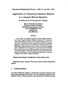
Fig.. 1: Absolute error for the 10th-order approximation by standard VIM for u ( x, t ) in example 3.1.

Fig.. 2: The h -curve of ∂u10 ( x, t , h) / ∂t given by (10) when x = 5 and t = 5 .

Fig.. 3: The error of norm 2 of r10 ( x, t , h) given

by (10) with respect to h in example 3.1.

Now, using the recursive scheme (5), we have

u0 ( x, t ) = u ( x,0) = sin( x) , u1 ( x, t , h) = sin( x) − h sin( x) t ,

Furthermore, according to (6) we define the residual function,

ISSN: 1565-1339 International Journal of Nonlinear Sciences & Numerical Simulation 11(7) 502-509, 2010

505

Fig.. 5: Absolute error for the 10th-order approximation by the standard VIM in example 3.2.

∂ u10 ( x, t , h) ∂ 4 u10 ( x, t , h) + r10 ( x, t , h) = ∂t ∂ x4 (9) for obtaining a suitable value of h . Fig. 3 shows the error of norm 2 of the residual function (9) for the 10th-order approximation, i.e.

⎛ 1 20 20 ⎛ ⎛ i j ⎞ ⎞ 2 ⎞ ⎜ ⎜⎜ r10 ⎜ , , h ⎟ ⎟⎟ ⎟ ⎜ (21) 2 ∑∑ ⎝ 2 2 ⎠ ⎠ ⎟⎠ i =0 j =0 ⎝ ⎝

1 2

(10)

with respect to h for ( x, t ) ∈ [0,10] × [0,10] . According to Figs. 2 and 3, we select h = 0.55 and the absolute error of u10 ( x, t ) reduces remarkably as shown in Fig. 4.

Example 3.2 Consider the following evolution equation [27]:

⎧ut + u x = 2 u xxt , ⎨ −x ⎩u ( x, 0) = e ,

t > 0, 0 ≤ x ≤ 10, 0 ≤ x ≤ 10. (11)

which admits the solution u ( x, t ) = e − x −t . We take the solution domain ( x, t ) ∈ [0,10] × [0,10] .

as

Similarly the absolute error of u10 ( x, t ) for

( x, t ) ∈ [0,10] × [0,10] tends to very large when time tends to 10, as illustrated in Fig.5. Using the iteration formulation, Eq.(5), we successively have

u 0 ( x, t ) = u ( x,0) = e − x , u1 ( x, t , h) = e − x + ht e − x , and in general, un +1 ( x, t , h) = un ( x, t , h)

Fig.. 4: Absolute error for the 10th-order approximation by the present technique when h = 0.55 in example 3.1

t ⎧ ∂ u ( x, s , h ) ∂ u ( x, s , h) ∂ 3 u n ( x, s , h ) ⎫ −h ∫ ⎨ n + n −2 ⎬ ds 0 ∂s ∂x ∂ x 2 ∂s ⎭ ⎩

We define the following residual function, r10 ( x, t , h) = −2

∂ u10 ( x, t , h) ∂ u10 ( x, t , h) + ∂t ∂x

∂ 3 u10 ( x, t , h) ∂ x 2 ∂t (12)

for obtaining suitable value of h . Fig. 6 shows the error of norm 2 of the residual function (12) for the 10th-order approximation, i.e.

506

XXXXXXX: Variational Iteration Method for Re-formulated Partial Differential Equations

⎛ 1 ⎜ ⎜ (21) 2 ⎝

⎛ ⎛ i j ⎞⎞ ⎜⎜ r10 ⎜ , , h ⎟ ⎟⎟ ∑∑ ⎝ 2 2 ⎠⎠ i =0 j =0 ⎝ 20

20

2

⎞ ⎟ ⎟ ⎠

1 2

(13)

with respect to h for ( x, t ) ∈ [0,10] × [0,10] . According to Fig. 6, we select h = −0.55 . The absolute error of u10 ( x, t ) in the solution domain ( x, t ) ∈ [0,10] × [0,10] is given in Fig. 7, the accuracy is remarkably improved by the optimal choice of h.

Example 3.3 Consider the following RLW equation [27]:

⎧ut − u xxt + u u x = 0, t > 0, 0 ≤ x ≤ 10, ⎨ 0 ≤ x ≤ 10. ⎩u ( x,0) = x ,

(14)

The exact solution of this problem is u ( x, t ) = x /(1 + t ) . Similarly we take the solution domain as ( x, t ) ∈ [0,10] × [0,4] . According to the standard VIM, we have the following variational iteration formula: un +1 ( x, t ) = un ( x, t ) t ⎧ ∂ u ( x, s ) ∂ 3 u n ( x, s ) ∂ u ( x, s ) ⎫ −∫ ⎨ n − + un ( x, s ) n ⎬ ds 2 0 ∂ x ∂s ∂x ⎭ ⎩ ∂s

u 0 ( x, t ) = u ( x,0) = x , we calculate the approximate solution till u 5 ( x, t ) .

Beginning with

The absolute error is shown in Fig.8, it is obvious that the same problem keeps unchanged.

Fig.. 6: The error of norm 2 of r10 ( x, t , h) given

with respect to h in example 3.2.

Fig.. 8: Absolute error for the 5th-order approximation by standard VIM in example 3.3

Now by the iteration algorithm, Eq.(5), we have

u 0 ( x, t ) = u ( x,0) = x , u1 ( x, t , h) = x − h x t , and in general, Fig.. 7: Absolute error for the 10th-order approximation by the present technique when h = −0.55 in example 3.2

ISSN: 1565-1339 International Journal of Nonlinear Sciences & Numerical Simulation 11(7) 502-509, 2010

un +1 ( x, t , h) = un ( x, t , h) − h ∫

t 0

507

∂ un ( x, s , h) ds ∂s

3 t ⎧ ∂ u ( x, s , h) ∂ u ( x, s , h ) ⎫ n −h ∫ ⎨− + u n ( x, s , h ) n ⎬ ds 2 0 ∂ x ∂s ∂x ⎩ ⎭

We define the residual function of u 5 ( x, t ) : ∂ u5 ( x, t , h) ∂ 3 u5 ( x, t , h) − ∂t ∂ x 2 ∂t ∂ u ( x, t , h ) + u5 ( x , t , h ) 5 ∂x

r5 ( x, t , h) =

(15)

for obtaining an optimal value of h . Fig.9 shows the error of norm 2 of the residual function (15) for 5th-order approximation, i.e.

⎛ 1 ⎜ ⎜ (31) 2 ⎝

⎛ ⎛ i 4 j ⎞⎞ ⎜⎜ r5 ⎜ , , h ⎟ ⎟⎟ ∑∑ ⎠⎠ i = 0 j = 0 ⎝ ⎝ 3 30 30

30

2

⎞ ⎟ ⎟ ⎠

1 2

Fig.. 10: Absolute error for the 5th-order approximation by the present technique when h = 0.43 in example 3.3.

5. Conclusion (16)

with respect to h for ( x, t ) ∈ [0,10] × [0,4] .

The present technology provides a simple way to adjust and control the convergence region of approximate solution for any values of t and x . An optimal auxiliary parameter can be obtained by the h -curve and the error of norm 2 of the residual function. Numerical results explicitly reveal the complete reliability, efficiency and accuracy of the suggested technique. It needs to be highlighted that the proposed variational iteration algorithm involving an auxiliary parameter is particularly suitable for inverse problems and differential-difference equations.

References

Fig.. 9: The error of norm 2 of r10 ( x, t , h) given

by (16) with respect to h in example 3.3. According to Fig.9, we select h = 0.43 . The absolute error reduces greatly for u 5 ( x, t ) ,

( x, t ) ∈ [0,10] × [0,4] as shown in Fig. 10.

[1] He JH. Variational iteration method - a kind of non-linear analytical technique: some examples, International Journal of Non-Linear Mechanics, 34 (4)(1999) 699-708 [2] He JH. Variational iteration method - some recent results and new interpretations, Journal of Computational and Applied Mathematics, 207(1)(2007): 3-17 [3] He JH, Wu XH. Variational iteration method: new development and applications, Computers & Mathematics with Applications, 54(2007): 881-894

508

XXXXXXX: Variational Iteration Method for Re-formulated Partial Differential Equations

[4] He JH. Non-perturbative methods for strongly nonlinear problems, Berlin: dissertation.de-Verlag im Internet GmbH, 2006 [5] He JH. Some asymptotic methods for strongly nonlinear equations, International Journal of Modern Physics B, 20 (10)(2006) 1141-1199 [6] He JH. An elementary introduction to recently developed asymptotic methods and nanomechanics in textile engineering, International Journal of Modern Physics B, 22(21)(2008): 3487-3578 [7] J. H. He, G. C. Wu and F. Austin, The variational iteration method which should be followed, Nonlin. Sci. Lett. A, 1 (2010), 1-30. E, Latifizadeh H. [8] Hesameddini Reconstruction of Variational Iteration Algorithms using the Laplace Transform, Int. J. Nonlin. Sci. Num., 10(2009): 1377-1382 [9] Salkuyeh DK. Convergence of the variational iteration method for solving linear systems of ODEs with constant coefficients, Computers & Mathematics with Applications, 56(2008): 2027-2033 [10] Khan NA, Ara A, Ali SA, et al. Analytical Study of Navier-Stokes Equation with Fractional Orders Using He's Homotopy Perturbation and Variational Iteration Methods, Int. J. Nonlin. Sci. Num., 10(2009): 1127-1134 [11] Ates I, Yildirim A. Application of variational iteration method to fractional initial-value problems, Int. J. Nonlin. Sci. Num., 10(2009): 877-883 [12] Das S. Solution of Fractional Vibration Equation by the Variational Iteration Method and Modified Decomposition Method, Int. J. Nonlin. Sci. Num., 9(2008): 361-366 [13] Goh SM, Noorani MSN, Hashim I, et al. Variational Iteration Method as a Reliable Treatment for the Hyperchaotic Rossler System, Int. J. Nonlin. Sci. Num., 10(2009): 363-371 [14] Chun C. Variational Iteration Method for a Reliable Treatment of Heat Equations

with Ill-defined Initial Data, Int. J. Nonlin. Sci. Num., 9(2008): 435-440 [15] Mokhtari R. Variational iteration method for solving nonlinear differential-difference equations, Int. J. Nonlin. Sci. Num., 9(2008): 19-23 [16] Saberi-Nadjafi J, Tamamgar M. The variational iteration method: A highly promising method for solving the system of integro-differential equations, Computers & Mathematics with Applications, 56(2008): 346-351 [17] Mokhtari R, Mohammadi M . Some Remarks on the Variational Iteration Method, Int. J. Nonlin. Sci. Num., 10(2009): 67-74 [18] Altintan D, Ugur O. Variational iteration method for Sturm-Liouville differential equations, Computers & Mathematics with Applications, 58(2009): 322-328 [19] Hemeda AA. Variational iteration method for solving wave equation, Computers & Mathematics with Applications, 56(2008) 1948-1953 [20] N. Herişanu and V. Marinca, A modified variational iteration method for strongly nonlinear problems, Nonlin. Sci. Lett. A, 1 (2) (2010), 183-192. [21] Noor MA, Mohyud-Din ST. Variational iteration method for solving higher-order nonlinear boundary value problems using He's polynomials, Int. J. Nonlin. Sci. Num., 9(2008): 141-156 [22] E. Yilmaz, M. Inc., Numerical simulation of the squeezing flow between two infinite plates by means of the modified variational iteration method with an auxiliary parameter, Nonlin. Sci. Lett. A, 1(3) (2010), 297-306. [23] Zayed EME, Rahman HMA. On solving the KdV-Burger's equation and the Wu-Zhang equations using the modified variational iteration method, Int. J. Nonlin. Sci. Num., 10(2009): 1093-1103 [24] Geng FZ, Cui MG. Solving Nonlinear Multi-point Boundary Value Problems by Combining Homotopy Perturbation and Variational Iteration Methods, Int. J. Nonlin. Sci. Num., 10(2009):597-600

ISSN: 1565-1339 International Journal of Nonlinear Sciences & Numerical Simulation 11(7) 502-509, 2010

[25] S. T. Mohyud-Din, M. A. Noor and K. I. Noor, Some relatively new techniques for nonlinear problems, Math. Prob. Eng. 2009 (2009), Article ID 234849, 25 pages, doi:10.1155/2009/234849. [26] M. M. Hosseini, S. T. Mohyud-Din, H. Ghaneai, On the coupling of auxiliary parameter, Adomian's polynomials and

509

correction functional, Math. Comput. Appl. (2010), In Press. [27] D. D. Ganji, Hafez Tari, M. Bakhshi Jooybari, Variational iteration method and homotopy perturbation method for nonlinear evolution equations, Comput. Math. Appl. 54 (2007) 1018–1027.