3 Web service availability: impact of recovery strategies and traffic models 61 ..... combine various types of information, a systematic and pragmatic modeling approach .... Security is a composition of the attributes: confidentiality, integrity and ...
N d’ordre : 2275
Année 2005
THÈSE préparée au Laboratoire d’Analyse et d’Architecture des Systèmes du CNRS en vue de l’obtention du Doctorat de l’Institut National Polytechnique de Toulouse Ecole doctorale : Systèmes Spécialité : Systèmes Informatiques par
Magnos MARTINELLO
Modélisation et évaluation de la disponibilité de services mis en œuvre sur le web - Une approche pragmatique Availability modeling and evaluation of web-based services A pragmatic approach
Soutenue le 4 novembre 2005 devant le jury : Président Directeur de thèse Rapporteurs Examinateurs
M. M. M. M. M. Mme.
Daniel Mohamed Yves András Nicolae Karama
NOYES KAÂNICHE DUTUIT PATARICZA FOTA KANOUN
Laboratoire d’Analyse et d’Architecture des Systèmes du CNRS 7, avenue du Colonel Roche, 31077 Toulouse Cedex 4
Rapport LAAS N 0000
In Memory of my grandmother Leocadia.
ii
Avant-propos Les travaux présentés dans ce mémoire ont été effectués au Laboratoire d’Analyse et d’Architecture des Systèmes du CNRS. Je remercie Messieurs Jean-Claude Laprie et Malik Ghallab, qui ont assuré la direction du LAAS-CNRS depuis mon entrée, de m’avoir accueilli au sein de ce laboratoire. Je remercie également Messieurs David Powell et Jean Arlat, Directeurs de Recherche CNRS, responsables successifs du groupe de recherche Tolérance aux fautes et Sûreté de Fonctionnement informatique (TSF), de m’avoir permis de réaliser mes travaux dans ce groupe. J’exprime ma profonde reconnaissance à Mohamed Kaâniche, Chargé de Recherche CNRS, pour avoir dirigé mes travaux de thèse, pour ses conseils, sa détermination impressionnante et notamment une méthodologie remarquable. Je suis également très reconnaissant à Karama Kanoun, Directeur de Recherche CNRS, pour ses orientations et ses critiques constructives. Je la remercie pour ses remarques pertinentes et pour avoir su canaliser mon énergie. J’ai tiré de nombreux enseignements de leur compétence et de leur expérience. Je remercie Monsieur Daniel Noyes, Professeur à l’École Nationale des Ingénieurs de Tarbes, pour l’honneur qu’il me fait en présidant mon jury de thèse, ainsi que: Monsieur Yves Dutuit, Professeur à l’Université de Bordeaux I Monsieur Nicolae Fota, Responsable du Pôle Safety à SOFREAVIA Monsieur Mohamed Kaâniche, Chargé de Recherche CNRS Madame Karama Kanoun, Directeur de Recherche CNRS Monsieur András Pataricza, Professeur à Budapest University of Technology and Economics
iii
iv pour l’honneur qu’ils me font en participant à mon jury. Je remercie tout particulièrement Messieurs Dutuit et Pataricza d’avoir accepté la charge d’être rapporteurs. Les travaux développés dans cette thèse ont été partiellement effectués dans le cadre du projet européen DSOS - Dependability Systems of Systems et financés en partie par la CAPES. J’exprime ma vive reconnaissance à la société brésilienne d’avoir soutenu mes études à travers la bourse de doctorat fournie par la CAPES. Je remercie vivement tous les membres du groupe TSF, permanents, doctorants et stagiaires. C’était un grand plaisir et je dirais un privilège d’échanger des idées, de discuter, de rigoler, enfin de vivre cette expérience parmi vous. J’associe à ces remerciements Joëlle, Gina et Jemina pour leur collaboration dans l’organisation de déplacements et, surtout, les derniers préparatifs de la soutenance. Les différents services techniques et administratifs du LAAS-CNRS, par leur efficacité et leur disponibilité, m’ont permis de travailler dans d’excellentes conditions. Je les remercie sincèrement. Il m’est impossible de ne pas mentionner le front philosophique de libération du bureau 20. J’ai trouvé de véritables compagnons de route qui ont su maintenir l’ambiance de travail plutôt décontractée et animée. Un grand merci à tous mes amis qui ont été toujours là, même virtuellement et avec qui j’ai partagé des moments formidables. Vous étiez une source de motivation et grâce à vous je me suis rechargé tout en gardant mon enthousiasme. Eu quero deixar um agradecimento especial à todos os brasileiros, latinos e agregados com quem eu pude passar vários momentos maravilhosos na França e fora da França. Eu posso dizer sinceramente que esta lista é enorme, e prefiro resumir dizendo que tive uma sorte imensa de encontrar pessoas como vocês, porque simplesmente vocês são fantásticos. Je remercie ma famille pour leur encouragement permanent, malgré l’océan qui nous sépare. Apesar de fisicamente estarmos distantes, vocês estiveram presentes em pensamento e graças à vocês eu cheguei onde cheguei. Enfin, mon amour, celle qui a tout partagé avec moi pendant ces années d’études. Robertinha, você é a minha fonte de inspiração e a pessoa mais especial deste mundo. Eu só posso te dizer do fundo do meu coração: obrigado por me amar.
Acknowledgments First of all, I would like to express my sincere gratitude to all the people who made this work together with me, participating intensively along these four years of adventure. Four years of intensive learning with a mix of excellent experiences and difficulties, but certainly a wonderful period of my live. My gratitude to the directors of the LAAS-CNRS, Jean-Claude Laprie and Malik Ghallab and also to David Powell and Jean Arlat the successive heads on dependable computing and fault tolerance research group (TSF), for their support allowing me to work in the best conditions. A very special thanks to the main responsibles of this adventure. Mohamed Kaâniche for being an advisor always ready to give all his energy with an inestimable determination and a remarkable methodology. Karama Kanoun for leading our discussions with her strategic vision, constant help and guidance in the research. I need to say that my multiple intrusions in their office were answered with availability and much attention. Moreover, the remarks and the way both conducted this work were not only fundamental to this thesis, but also they had a special value for me in the process of formation. My sincere thanks to the people of group TSF with whom I had the pleasure of interacting and collaborating not only on technical aspects but specially personally. I think the most important lesson learned is how to do scientific research. Special thanks go to my friends. For me, you are like brothers and sisters and an incredible source of motivation. Finally, I thank my family for their love and support during these years of study. My parents Darci and Silvia two of the most wonderful people in the world. Tiago and Diego who are fantastic brothers. My wife Robertinha, who is my inspiration and the most special person in the world. I just thank you from the bottom of my heart for loving me.
v
vi
Contents Introduction
1
1 Context and background
7
1.1 Context and motivation . . . . . . . . . . . . . . . . . . . . . . . . . .
7
1.2 Dependability concepts . . . . . . . . . . . . . . . . . . . . . . . . . . .
8
1.3 Dependability evaluation . . . . . . . . . . . . . . . . . . . . . . . . . .
9
1.4 Modeling process
. . . . . . . . . . . . . . . . . . . . . . . . . . . . .
11
1.4.1 Dependability measures . . . . . . . . . . . . . . . . . . . . . .
13
1.4.2 Model construction . . . . . . . . . . . . . . . . . . . . . . . . .
14
1.4.3 Model solution . . . . . . . . . . . . . . . . . . . . . . . . . . .
16
1.4.4 Model validation . . . . . . . . . . . . . . . . . . . . . . . . . .
16
1.5 Dealing with large models . . . . . . . . . . . . . . . . . . . . . . . . .
17
1.6 Related work on web evaluation . . . . . . . . . . . . . . . . . . . . . .
19
1.6.1 Measurements based evaluation . . . . . . . . . . . . . . . . . .
19
1.6.2 Modeling based evaluation . . . . . . . . . . . . . . . . . . . .
22
1.7 Conclusion . . . . . . . . . . . . . . . . . . . . . . . . . . . . . . . . .
23
2 Availability modeling framework
25
2.1 Problem statement . . . . . . . . . . . . . . . . . . . . . . . . . . . . .
26
2.2 Dependability framework . . . . . . . . . . . . . . . . . . . . . . . . .
28
2.2.1 User level . . . . . . . . . . . . . . . . . . . . . . . . . . . . . .
28
2.2.2 Function level . . . . . . . . . . . . . . . . . . . . . . . . . . . .
31
2.2.3 Service Level . . . . . . . . . . . . . . . . . . . . . . . . . . . .
31
2.2.4 Resource level
. . . . . . . . . . . . . . . . . . . . . . . . . . .
32
2.2.5 Availability modeling . . . . . . . . . . . . . . . . . . . . . . . .
34
vii
CONTENTS
viii
2.3 Travel Agency (TA) description . . . . . . . . . . . . . . . . . . . . . .
36
2.3.1 Function and user levels . . . . . . . . . . . . . . . . . . . . . .
37
2.3.2 Service and function levels
. . . . . . . . . . . . . . . . . . . .
40
. . . . . . . . . . . . . . . . . . . . . . . . . . .
45
2.4 TA availability modeling . . . . . . . . . . . . . . . . . . . . . . . . . .
46
2.4.1 Service level availability . . . . . . . . . . . . . . . . . . . . . .
46
2.3.3 Resource level
2.4.1.1
External services . . . . . . . . . . . . . . . . . . . . .
46
2.4.1.2
Internal services . . . . . . . . . . . . . . . . . . . . .
47
2.4.2 Function level availability . . . . . . . . . . . . . . . . . . . . .
51
2.4.3 User level availability
. . . . . . . . . . . . . . . . . . . . . . .
53
2.5 Evaluation results . . . . . . . . . . . . . . . . . . . . . . . . . . . . . .
53
2.5.1 Web service availability results . . . . . . . . . . . . . . . . . .
54
2.5.2 User level availability results . . . . . . . . . . . . . . . . . . .
56
2.6 Conclusion . . . . . . . . . . . . . . . . . . . . . . . . . . . . . . . . .
57
3 Web service availability: impact of recovery strategies and traffic models 61 3.1 Introduction . . . . . . . . . . . . . . . . . . . . . . . . . . . . . . . . .
62
3.2
63
Fault tolerance strategies in web clusters
. . . . . . . . . . . . . . . .
3.2.1 Non Client Transparent (NCT) recovery strategy
. . . . . . . .
63
3.2.2 Client Transparent (CT) recovery strategy . . . . . . . . . . . .
64
3.3 Modeling assumptions . . . . . . . . . . . . . . . . . . . . . . . . . . .
65
3.4
. . . . . . . . . . . . . . . . . . . . . . . . . . . . .
67
3.4.1
Availability model . . . . . . . . . . . . . . . . . . . . . . . . .
67
3.4.2
Performance model . . . . . . . . . . . . . . . . . . . . . . . .
68
3.4.2.1
Poisson Process Traffic . . . . . . . . . . . . . . . . .
68
3.4.2.2
Markov Modulated Poisson Process Traffic . . . . . .
69
Cluster Modeling
3.4.3
Composite Availability - Performance model
��
3.4.3.1
Loss probability due to buffer overflow
3.4.3.2
Loss probability due to server node failure
3.4.3.3
70
. . . . .
71
�� �
. .
72
Loss probability during the node failure detection time �� ..........................
72
Summary
. . . . . . . . . . . . . . . . . . . . . . . .
74
Evaluation Results . . . . . . . . . . . . . . . . . . . . . . . . . . . . .
74
3.5.1
77
3.4.3.4 3.5
. . . . . . . . . .
Sensitivity to MTTF . . . . . . . . . . . . . . . . . . . . . . . .
CONTENTS
3.6
ix
3.5.2
Sensitivity to MTTD . . . . . . . . . . . . . . . . . . . . . . . .
78
3.5.3
Sensitivity to service rate . . . . . . . . . . . . . . . . . . . . .
78
3.5.4
Impact of traffic model . . . . . . . . . . . . . . . . . . . . . .
80
3.5.4.1
Sensitivity to traffic burstiness . . . . . . . . . . . . .
82
3.5.4.2
Load effects on �� . . . . . . . . . . . . . . . . . . .
84
Conclusion . . . . . . . . . . . . . . . . . . . . . . . . . . . . . . . . .
85
4 Service unavailability due to long response time
87
4.1
Availability measure definition . . . . . . . . . . . . . . . . . . . . . .
88
4.2
Single server queueing systems
. . . . . . . . . . . . . . . . . . . . .
90
Modeling unavailability due to long response time . . . . . . .
90
4.2.1.1
Conditional response time distribution . . . . . . . . .
90
4.2.1.2
Service availability modeling . . . . . . . . . . . . . .
91
4.2.1
4.2.2
Sensitivity analysis
. . . . . . . . . . . . . . . . . . . . . . . .
92
4.2.2.1
Variation of response time . . . . . . . . . . . . . . . .
92
4.2.2.2
Effects of � and � on �� . . . . . . . . . . . . . . . .
94
4.2.2.3
95
Multi-server queueing systems . . . . . . . . . . . . . . . . . . . . . .
97
4.3.1
Modeling unavailability due to long response time . . . . . . .
97
4.3.1.1
Conditional response time distribution . . . . . . . . .
97
4.3.1.2
Service availability modeling . . . . . . . . . . . . . .
98
4.3.2
Sensitivity analysis
. . . . . . . . . . . . . . . . . . . . . . . . 100
4.3.2.1
Variation of response time distribution . . . . . . . . 100
4.3.2.2
Load effects on �� . . . . . . . . . . . . . . . . . . . 101
4.3.2.3 4.3.2.4 4.4
95
Approximation for �� . . . . . . . . . . . . . . . . . .
4.2.2.4 4.3
Finite buffer effects on �� . . . . . . . . . . . . . . .
Impact of aggregated service rate on �� . . . . . . . 102 Impact of the number of servers on �� . . . . . . . 103
Conclusion . . . . . . . . . . . . . . . . . . . . . . . . . . . . . . . . . 103
Conclusion
105
Appendix I
109
Appendix II
119
Bibliography
127
x
CONTENTS
List of Figures 1
Interdependence of chapters
. . . . . . . . . . . . . . . . . . . . . . .
3
1.1 A simplified view of the modeling process and its interactions with measurement based evaluation . . . . . . . . . . . . . . . . . . . . . .
12
2.1 Three key players of a web based system . . . . . . . . . . . . . . . . .
26
2.2 Hierarchical availability modeling framework . . . . . . . . . . . . . .
29
2.3 User’s operational profile . . . . . . . . . . . . . . . . . . . . . . . . . .
30
2.4 An example of Interaction diagram associated to a function . . . . . .
32
2.5 Example of configurations for a Web server
. . . . . . . . . . . . . . .
34
2.6 TA high-level structure . . . . . . . . . . . . . . . . . . . . . . . . . . .
36
2.7 User operational profile graph . . . . . . . . . . . . . . . . . . . . . . .
38
2.8 Interaction diagram of the Browse function . . . . . . . . . . . . . . .
43
2.9 Interaction diagram of the Search function . . . . . . . . . . . . . . . .
44
2.10 Interaction diagram of the Book function . . . . . . . . . . . . . . . . .
44
2.11 Interaction diagram of the Pay function . . . . . . . . . . . . . . . . . .
44
2.12 Basic architecture . . . . . . . . . . . . . . . . . . . . . . . . . . . . . .
45
2.13 Redundant architecture . . . . . . . . . . . . . . . . . . . . . . . . . .
46
2.14 Perfect coverage model . . . . . . . . . . . . . . . . . . . . . . . . . . .
49
2.15 Imperfect coverage model . . . . . . . . . . . . . . . . . . . . . . . . .
50
2.16 Web service unavailability with perfect coverage . . . . . . . . . . . . .
55
2.17 Web service unavailability with imperfect coverage . . . . . . . . . . .
55
2.18 User perceived unavailability with ��
. . . . . . . . . . . . . . .
58
3.1 Basic web cluster architecture . . . . . . . . . . . . . . . . . . . . . . .
66
3.2 Availability model of the web cluster . . . . . . . . . . . . . . . . . . .
68
xi
� �
LIST OF FIGURES
xii
3.3 A web cluster with � servers available and load balancing . . . . . . .
69
3.4 Markov Modulated Poisson Process modeling the request arrival process 70 3.5 Impact of MTTF on �� . . . . . . . . . . . . . . . . . . . . . . . . . .
3.6 Impact of failure detection duration on �� for both recovery strategies
77 79
3.7 Impact of service rate on �� . . . . . . . . . . . . . . . . . . . . . .
80
3.8 MMPP traffic models representing the traffic distribution along the day
81
3.9 Effects of the traffic burstiness on �� for both recovery strategies . . .
83
3.10 Effects of service load � on �� . . . . . . . . . . . . . . . . . . . . . . 4.1 4.2 4.3 4.4 4.5 4.6
� �� � � �� variation for single server queueing system . . . . . �� for an M/M/1 queue system model as a function of � . . . . �� for an M/M/1 queue system model as a function of � . . . . . The effect of finite buffer size � on �� . . . . . . . . . . . . . . . �� as a function of � using equation (4.8) and equation (4.11) � ��� � � �� variation for multi-server queuing systems . . . . .
84
. . .
93
. . .
94
. . .
95
. . .
96
. . .
97
. . . 101
List of Tables 2.1 Examples of functions provided by e-Business web sites . . . . . . . . .
31
2.2 TA user scenarios with associated probabilities �� . . . . . . . . . . . .
39
2.3 Profile of user class A
. . . . . . . . . . . . . . . . . . . . . . . . . . .
40
2.4 Profile of user class B
. . . . . . . . . . . . . . . . . . . . . . . . . . .
41
2.5 User scenario probabilities (in %) . . . . . . . . . . . . . . . . . . . . .
41
2.6 Scenario categories for user classes A and B . . . . . . . . . . . . . . .
41
2.7 Mapping between functions and services . . . . . . . . . . . . . . . . .
42
2.8 External service availability . . . . . . . . . . . . . . . . . . . . . . . .
47
2.9 Application and database service availability
. . . . . . . . . . . . . .
47
. . . . . . . . . . . . . . . . . . . . . . . . . .
52
2.11 Function level availabilities . . . . . . . . . . . . . . . . . . . . . . . .
53
2.12 Numerical values of the model parameters
. . . . . . . . . . . . . . .
56
2.13 User availabilities for classes A and B . . . . . . . . . . . . . . . . . . .
56
3.1 Closed-form equations for NCT recovery strategy . . . . . . . . . . . .
75
3.2 Closed-form equations for CT recovery strategy . . . . . . . . . . . . .
76
3.3 Numerical values of the model parameters
. . . . . . . . . . . . . . .
76
3.4 The MMPP models and traffic burstiness . . . . . . . . . . . . . . . . .
82
4.1 Closed-form equations for single server queueing systems . . . . . . .
92
4.2 Effects on �� as � increases for � � ���
. . . . . . . . . . . . . . . .
94
4.3 Closed-form equations for multi-servers queueing systems . . . . . . .
99
2.10 Web service availability
4.4 Configurations for an aggregated service rate of � � � requests/sec. 100 4.5 4.6 4.7
�� for an aggregated service rate of � � � requests/sec. �� for an aggregated service rate of � � requests/sec. �� in days:hours:minutes per year for � � ���. . . . . . . . xiii
. . . . . . 102 . . . . . . 102 . . . . . . 103
xiv
LIST OF TABLES
Introduction Deal with the faults of others as gently as with your own. Chinese proverb
O
the past years, the Internet has become an huge infrastructure used daily by millions of people in the world. The world wide web (www or web) is a publishing medium used to disseminate information quickly through this infrastructure. The web has had a rapid growth in size and usage, with an extensive development of web sites delivering a large variety of personal, commercial and educational material. Virtual stores on the web allow to buy books, cds, computers, and many other products and services. New web applications such as e-commerce, digital libraries, video on-demand and distance learning make the issue of dependability evaluation increasingly important, in particular with respect to the service perceived by web users. VER
Businesses and individuals are increasingly depending on web-based services for any sort of operations. Web-based services 1 connect departments within organizations, multiple companies and the population in general. In addition, the web is often used for critical applications such as online banking, stock trading, booking systems requiring high availability and performance of the service. In those applications, a temporary service unavailability may have unacceptable consequences in terms of financial losses. A period of service unavailability may cost millions to the site depending on the duration and on the importance of the period 2 . It may be very difficult to access a major newspaper or TV site after some important news due to site overload. Those periods are usually most important to the web service provider because unplanned 1 In this thesis, web services refer to the services delivered by a web application. Such services do not refer to the standards and protocols proposed by W3C and OASIS (both responsible for the architecture and standardization of web services). 2 According to [Patterson et al. 2002] well-managed servers today achieve an availability of 99.9% to 99%, or equivalently between 8 to 80 hours of downtime per year. Each hour can be costly e.g. $200,000 per hour for Amazon.
1
unavailability is more expensive than planned unavailability [Brewer 2001]. For instance, ebay web site was unavailable for a period of 22 hours on June 1999, leading to a lost revenue of approximatively 5 billion dollars. Dependability analysis and evaluation methods are useful to understand, analyze, design and operate web-based applications and infrastructures. Quantitative measures need to be evaluated in order to estimate the quality of service and the reliance that can be placed on the provided service. This evaluation may help web site designers to identify the weak parts of the architecture which can be used for improving the provided service. Dependability evaluation consists in estimating quantitative measures allowing to analyze how hardware, software or human related failures affect the service dependability. It can be carried out by dependability modeling with the goal of analyzing the various design alternatives in order to choose the final solution that better satisfies the requirements. Evaluation can be carried out using two complementary approaches: i) measurement and ii) modeling. Measurements provide information for characterizing the current and past behavior of already existing systems. Recently, much research effort has been devoted to the analysis of service availability using measurements based on monitoring of operational web sites. On the other hand, it is fundamental to anticipate future behavior about the infrastructure supporting the service. Modeling is useful to guide the development of a web application during its design phase by providing quantitative measures characterizing its dependability. In the context of web-based services, modeling has been mainly used for performance evaluation purposes. However, less attention has been devoted to the dependability modeling and evaluation of web-based services and applications, specially from the user perceived perspective. The user perceived availability of web-based services is affected by a variety of factors (e.g., user behaviors and workload characteristics, fault tolerance and recovery strategies, etc.). Due to the complexity of the web-based services and the difficulty to combine various types of information, a systematic and pragmatic modeling approach is needed to support the construction and processing of dependability models. The contributions presented in this thesis are aimed at fulfilling these objectives, introducing a pragmatic approach for analyzing the availability of such services from the user point of view. The traditional notion of availability is extended in order to include some of the main causes of service unavailability relying on a performability modeling approach. Our modeling approach is based on a combination of Markov reward models and queuing theory, in which we investigate the potential existing closed-form equations. In fact, analysis from pure performance viewpoint tends to be optimistic because it ignores the failure/repair behavior of the system. On the other hand, pure dependability analysis that does not include performance levels of service delivery tends to be too conservative. Therefore, a performability based approach is well suited to capture the various degraded states, measuring not only whether the service is up or down but also operational degraded states. The causes of service unavailability considered explicitly in our modeling based approach fall into the following categories: i) hardware and
2
software failures affecting the servers; and ii) performance-related failures including: overload, loss of requests, and long response time.
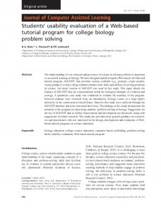
����� ��� � � The core of this thesis deals with web service availability modeling and evaluation and is structured in four chapters. Figure 1 presents the interdependence of chapters.
Introduction
Chapter 1 Context and background
Chapter 2 Availability modeling framework
Chapter 3
Chapter 4 Service unavailability due to long response times
Web service availability: impact of recovery strategies and traffic models
Appendix I
Appendix II
Proofs and implementation
Proofs and implementation
Conclusion Figure 1: Interdependence of chapters
3
Chapter 1 states the motivation and the context of the work. It briefly presents the theory and techniques for dependability modeling providing a background for our investigation. We provide a discussion on dependability modeling starting by the main concepts of dependability. A brief overview of dependability evaluation is presented with some existing methods useful to build and to solve models. Some approaches in the probabilistic evaluation domain are reported. Also, the related works are reviewed presenting prior studies and contributions on web availability evaluation including measurements and modeling approaches. The general problem addressed in this thesis is introduced in Chapter 2. This chapter presents the proposed framework using a web-based travel agency as example, illustrating the main concepts and the feasibility of the framework. The framework is based on the decomposition of the web based application following a hierarchical description. The hierarchical description is structured into four levels of abstraction. The highest level describes the dependability of the web application as perceived by the users. Intermediate levels describe the dependability of functions and services provided to the users. The lowest level describes the dependability of the component systems on which functions and services are implemented. Sensitivity analyses are presented to show the impact of users operational profile, the fault coverage and the travel agency architecture on user perceived unavailability. Chapter 3 provides a modeling based approach of web service availability supported by web cluster architectures. We are particularly interested in fault-tolerant web architectures. Our interest is justified by the fact that web clusters architectures are leading architectures for building popular web sites. Web designers require to find an adequate sizing of these architectures to ensure high availability and performance for the delivered services. Moreover, it is crucial to study the impact of recovery strategies supported by these architectures on web service availability. Thus, we address especially recovery strategies issues and traffic burstiness effects on web service availability. Web cluster architectures are studied taking into account the number of nodes, recovery strategies after a node failure and the reliability of the nodes. Various causes of request loss are considered explicitly in the web service availability measure: losses due i) to buffer overflow or ii) to node failures, or iii) during recovery time. Closed-form equations for request loss probability are derived for both recovery strategies. Two simple traffic models (Markov Modulated Poisson Process (MMPP) and Poisson) are used to analyze the impact of traffic burstiness on web service availability. From the user perspective, the service is perceived as degraded or even unavailable if the response time is too long compared to what the users are expecting. Certainly, the long response time has an impact on the overall service availability. To our knowledge, however, there has not been a quantitative evaluation of the long response time effects on service availability especially from the web user perspective. Chapter 4 introduces a flexible analytic modeling approach for computing service unavailability due to long response times. The proposed approach relies on Markov reward models and queuing theory. We introduce a mathematical abstraction that is general enough
4
��� �� ��� �
to characterize the unavailability behavior due to long response times. The computation of the service unavailability measure is based on the evaluation of the response time distribution. Closed-form equations are derived for conditional response-time distribution and for the service unavailability due to long response time, considering single and multi-server queueing systems. The developed models are implemented using tools such as gnu-octave and maple. Since we specifically focus on small models aiming to obtain closed-form equations as much as possible, these tools are enough for evaluating the obtained equations and for supporting the sensitivity analyses. Appendix I and II show the obtained equations proofs as well as the models implementation of the chapters 3 and 4.
�
��� �� ��� �
�
Chapter 1
Context and background All models are wrong. Some models are useful. Albert Einstein
T
chapter presents the motivation and the context of our work. We provide a discussion on dependability evaluation starting by the main concepts of dependability. A brief overview of dependability evaluation is presented through some existing methods useful to build and to solve models. Various approaches used in probabilistic evaluation domain are non-exhaustively reported, illustrating the considerable advances that have extended the capabilities of analytic models. HIS
We introduce the modeling process indicating its phases. The phases are described presenting some of the main problems and methods used in each phase. After that, two major problems related to models construction and processing are discussed: largeness and stiffness. We report some approaches useful to build large models. Finally, we review the related studies that form the basis for our investigation on web availability evaluation including measurements and modeling approaches.
�
������� � ��� � �� The web is an evolving system incorporating new components and services at a very fast rate. A large number of new applications such as e-commerce, digital libraries, video on-demand, distance learning have been migrated to the web. Many web site projects are built in three or four months because they need to beat competitors and quickly establish a web presence. This requirement of becoming visible online often
7
�� � �� ��� �� ��� �� �� ����
comes without a careful design and testing, leading to some problems on dependability and performance. Recently, many high-tech companies providing service on the web have experienced operational failures. Financial web services experienced intermittent outages as the volume of visitors has increased. A report presented in [Meehan 2000] showed that online brokerage companies were concerned with system outages and with the inability to accommodate growing numbers of online investors. During those outages, users and investors could not access real-time quotes. Such operational problems have resulted, in many cases, in degraded performance, unsatisfied users and heavy financial losses. Quantitative methods are needed to understand, analyze, design and operate such large infrastructure. Quantitative measures need to be evaluated in order to estimate the quality of service and the reliance that can be placed on the provided service. This evaluation may help system designers to identify the weak parts of the system that should be improved to support an acceptable dependability level for the provided service. Dependability evaluation consists in estimating quantitative measures allowing to analyze how hardware, software or human related failures affect the system dependability. It can be carried out by dependability modeling with the goal of analyzing the various design alternatives in order to choose the final solution that better satisfies the requirements. The rest of this chapter is structured as follows. Section 1.2 presents the main concepts of dependability. Section 1.3 outlines the main approaches that can be used for dependability evaluation. Section 1.4 reports some formalisms and tools used in the analytic modeling process. Section 1.5 describes some of the main problems related to large models and the existing techniques to deal with large models. Section 1.6 presents the related work on the evaluation of web-based services. Finally, section 1.7 summarizes the chapter.
��
����� � � �� �������� Dependability is defined as the trustworthiness of a computer system such that reliance can justifiably be placed on the service it delivers [Laprie 1995, Laprie et al. 1996, Avizienis et al. 2004]. It is a global concept which includes various notions that can be grouped into three classes: threats, means and attributes. Dependability goal is to specify, conceive and investigate systems in which a fault is natural, predictable and tolerable. The threats to dependability are: faults, errors and failures; they are undesired - but not in principle unexpected - circumstances causing or resulting from undependability. The means for dependability are: fault prevention, fault tolerance, fault removal and fault forecasting or prediction; these are the methods and techniques that enable one
�
���� � ����� ��� �� ������
a) to provide the ability to deliver a service on which reliance can be placed, and b) to reach confidence in this ability. The attributes of dependability are: availability, reliability, safety, confidentiality, integrity, maintainability and security. Reliability: continuity of correct service; Availability: readiness for correct service; Safety: absence of catastrophic consequences on the user(s) and the environment; Confidentiality: absence of unauthorized disclosure of information; Integrity: absence of improper system alterations; Maintainability: ability to undergo modifications and repairs; Security is a composition of the attributes: confidentiality, integrity and availability requiring the concurrent existence of a) availability for authorized actions only, b) confidentiality, and c) integrity with ’improper’ meaning ’unauthorized’. In this study, we concentrate our attention on the fault forecasting domain taking into account only accidental faults. Fault forecasting is conducted by performing an evaluation of the system behavior with respect to fault occurrence or activation. Evaluation aims to estimate the presence, the creation and the consequences of faults or errors on dependability.
��
����� � � �� � �� � �� Fault forecasting is performed using evaluations of the behavior of a system relative to the occurrence of faults and their activation. By adopting a structural view of a system, evaluation consists in reviewing and analyzing the failures of its components and their consequences on the system’s dependability. Evaluation can be conducted in two ways [Laprie et al. 1996]: Ordinal evaluation: aims to identify, list and rank failures, or the methods and techniques implemented to avoid them; Probabilistic evaluation: aims to evaluate in terms of probabilities the degree of satisfaction of certain attributes of dependability; The probabilistic evaluation is basically carried out using two complementary approaches: i) measurement based evaluation and ii) modeling based evaluation. In the area of measurement, it is possible to distinguish two techniques:
�
�� � �� ��� �� ��� �� �� ����
Fault injection: consists in injecting faults in a target system which is usually not operational, aiming to speed up its behavior in the presence of faults [Arlat et al. 1993]. This technique is based on controlled experiments which are subjected to a given workload; Operational observation: consists in collecting data characterizing the behavior of a target system during its operational execution. The estimation of the dependability measures is based on the statistical processing of failure and recovery events extracted from the data. Such analysis can be carried out based on the error logs maintained by the operating system [Simache & Kaâniche 2002, Simache 2004]; Measurements provide the most accurate information on already existing systems, although sometimes it is difficult to ensure by measurements that a system meets the dependability requirements. For example, in the case of highly reliable systems waiting for the system to fail enough times to obtain statistically significant samples would take years. Nevertheless, measurements data can be used for model validation, for instance to calibrate the input of the model parameters. In the case of a system that does not exist yet, the parameters could be estimated from measurements on similar systems. Consequently, the better is to combine both measurement and modeling as much as possible. Modeling is useful to guide the development of the target system during the design phase by providing quantitative measures characterizing its dependability. Various design alternatives can be analyzed in order to choose the final solution that better satisfies the requirements. In particular, models can enable the designers i) to understand the impact of various design parameters from the dependability point of view, ii) to identify potential bottlenecks, iii) to aid in upgrade studies. These reasons make the modeling attractive in the probabilistic evaluation. We can distinguish essentially two main modeling techniques: simulation and analytical modeling. Discrete-event simulation can be applied to almost all problems of interest, but the main drawback is that it can take a long time to run, mainly for large and realistic systems with high accuracy. In particular, it is not trivial to simulate with high confidence scenarios mainly in the presence of rare events [Heidelberger 1995, Heidelberger et al. 1992], even if rare events can be speeded up in a controlled manner using for example importance sampling techniques [Nicola et al. 1990]. A designer faces many issues that should be considered at the same time when choosing an adequate method. Simplicity, accuracy, computational cost and availability of information about the system under study are some factors that can be used to determine the well-suited method. Analytic-based approach favors simplicity allowing to cover essential aspects of the target system. Indeed, analytical models can be a costeffective alternative to provide relatively quick answers to ”what-if” questions giving more insights for the system being studied.
��
���� ��� ��� � ��
Clearly, analytical models often use simplifying assumptions in order to make them tractable. However, considerable advances have extended the capabilities of analytic models. Our work explores how analytic-based models can be used for dependability evaluation of web-based services.
��
�� �� �� ������� In the modeling process, it is possible to identify the major phases as well as the interdependencies among the phases. A modeling process can be structured basically into four phases as shown in the right side of Figure 1.1: choice of measures, model construction, model solution and model validation. The choice of measures consists in determining the measures of predominant importance reflecting the evaluation objective according to system characteristics and application context. The application context determines the type of information that should be represented. Also, there are certain requirements that are directly related to the choice of measures. System requirements can be defined as the desired qualities explicitly or implicitly specified that need to be taken into account. The second step consists in selecting the most adapted modeling technique allowing the evaluation of the desirable measures and the building of an adequate model. This step is referred to as model construction. Once a suitable model has been developed, we need to solve the model. Model solution corresponds to the computation of the model in order to evaluate the measures, e.g. in terms of probabilities. Model validation is the task of checking model assumptions and its correctness. It is executed in an iterative process involving experts trying to reach consensus into the validation of the model assumptions and results. Whenever possible, the computed measures should be compared against operational measures obtained from measurement based evaluation executed in a real environment as indicated in Figure 1.1. The measurement results are used not only for model validation but also for providing numerical values for the model parameters.
��
�� � �� ��� �� ��� �� �� ����
Measurement based evaluation
Modeling based evaluation Modeling environment
Real environment
Choice of measures Target System
Model construction
Measurements
Model Solution
Operational measures
Compare
Computed measures Model Validation
Figure 1.1: A simplified view of the modeling process and its interactions with measurement based evaluation
��
���� ��� ��� � ��
� � ���� ���� ��� �������� The life of a system is perceived by its user(s) as an alternation between two states of the delivered service relative to the accomplishment of the system function: Correct service, where the delivered service accomplishes the system function; Incorrect service, where the delivered service does not accomplish the system function; A service failure is an event that occurs when the delivered service deviates from correct service. A service failure is thus a transition from a state of correct service to a state of incorrect service. In contrast, the transition from incorrect to a correct service is a restoration. The period of delivery of incorrect service is an outage. Quantifying the alternation of correct-incorrect service enables some measures of dependability to be defined [Avizienis et al. 2004]: Reliability: a measure of the continuous delivery of correct service or, equivalently the time to failure; Availability: a measure of the delivery of correct service with respect to the alternation of correct and incorrect service. In other words, the system alternates through periods in which it is operational - the up periods - and periods in which it is down - the down periods; Maintainability: a measure of the time to restoration since the last failure, or equivalently, the continuous delivery of an incorrect service; However, a system might have various modes of service delivery. These modes can be distinguished, ranging from full capacity to complete interruption going through different states of degradation. The modes can be classified as correct or incorrect according to the service requirement of the applications. From the dependability evaluation point of view, it is possible to consider two classes of systems: Degradable systems for which there are several modes of service delivery; Non-degradable systems that have only one mode of service delivery; Fault-tolerant systems supporting recovery strategies with service restoration are examples of degradable systems. Such systems are usually capable of providing multi modes of service delivery achieving acceptable levels of performance (multiperforming systems). Dependability evaluation of those systems can be carried out considering different classes of service degradation. It is important to notice that modeling any system with either a pure performance model or a pure dependability model can lead to incomplete or even misleading results. Analysis from pure performance viewpoint tends to be optimistic since it ignores
��
�� � �� ��� �� ��� �� �� ����
the failure/repair behavior of the system. On the other hand, pure dependability analysis taking into account system component failures tends to be too conservative if it does not consider the performance levels related to different modes of service delivery. The combination of performance related measures and dependability measures is usually called performability [Meyer 1980, Meyer 1982], which is well suited to evaluate the impact of service degradation on system dependability. It allows to consider the performance of a given system based on its different modes of service delivery. Performability measures characterize the ability of fault-tolerant systems to perform certain tasks in the presence of failures, taking into account component failures and performance degradation. In the following sections, we discuss in more details some of the main problems and methods used in model construction, solution and validation phases.
� � ���� �� ��������
Model construction is usually based on analytical or graphical description of the system behavior. Either information about a real computer system is used to build the model, or experiences gained in earlier modeling studies are implicitly used. Certainly, this process is rather complicated and it needs both modeling and system expertise. Analytical modeling has proved to be an attractive technique. A model is an abstraction of a system that includes sufficient details to facilitate the understanding of the system behavior. Analytical models can be classified into state space models (e.g. Markov chains and extensions) and non-state space models (e.g. fault trees, reliability block diagrams and reliability graphs). Non-state space models are commonly used to study system dependability [Vesely et al. 1981, Trivedi 2002, Dutuit & Rauzy 2000, Dutuit & Rauzy 1998]. They are concise, easy to understand, and have efficient solution methods. However, features such as non-independent behavior of components, imperfect coverage, and combination with performance can not be captured easily by these models. In the performance modeling, examples of non-state space models are precedence graphs (see the book [Roche & Schabes 1997] for a formal definition) and product form queueing networks [Jackson 1963]. A precedence graph is a directed and acyclic graph that can be used to model concurrency for the case of unlimited resources. On the other hand, contention for resources can be represented by a class of queueing networks known as product form queueing networks, for which there are efficient solution methods [Buzen 1973, Baskett et al. 1975, Reiser & Lavenberg 1980] allowing to derive steady state performance measures. However, they cannot model concurrency, synchronization, or server failures, since these violate the product form assumptions [Popstojanova & Trivedi 2000]. State space models enable us to overcome the limitations of the non-state space models by modeling complicated interactions among the components taking into
��
���� ��� ��� � ��
account the stochastic dependencies [Rabah & Kanoun 2003, Fota et al. 1999]. Also, they allow evaluation of different measures of interest. This evaluation can provide useful tradeoffs. Markov chains are the state space models most commonly used for modeling purposes. They provide great flexibility for modeling dependability, performance, and combined dependability and performance measures. Markov chains can also have rewards assigned to states or to transitions between states of the model. Reward structures refine the possibilities of evaluation. Markov reward models have been used in Markov decision theory to assign cost and reward structures to states [Howard 1971a]. Meyer [Meyer 1980] adopted Markov reward models to provide a framework for an integrated approach to allow combined performance and dependability evaluation. By extension, it is equally well-suited to the evaluation of systems with several modes of service delivery, notably through the computation of performability type measures. In practice, modeling tools have been developed to deal with Markov reward models. For instance, TANGRAM-II [Carmo et al. 1998] supports performability-oriented analysis using object-oriented language [Berson et al. 1991]. Petri nets and their extensions (e.g. stochastic Petri nets, reward Petri nets) represent another formalism extensively used for model construction [Florin & Natkin 1985]. They provide a higher-level model specification from which a Markov chain is generated. When model specification becomes too complex (i.e., models become huge to handle manually), it is necessary to use a modeling tool. In the case of Petri nets and their extensions, there are a number of tools suitable for modeling and evaluation. Among these tools are the following: SURF2 [C.Béounes et al. 1993], SPNP [Ciardo et al. 1989], ULTRASAN [Couvillion et al. 1991] and DEEM [Bondavalli et al. 2000]. In addition to Petri nets, recent research studies have focused on the generation of dependability models from high level specification formalisms and languages such as UML [Bondavalli et al. 2001a, Pataricza 2002, Majzik & Huszerl 2002], ALTARICA [Signoret et al. 1998] and AADL [Rugina et al. 2005, Rugina 2005]. The objective is to integrate dependability modeling into the industrial development processes. It is achieved by i) the enrichment of the functional specification and design models with dependability related informations and assumptions and ii) the definition of transformation rules allowing to generate dependability evaluation models (fault trees, GSPNs, Markov chains) from the enriched model. In this dissertation, we rely on Markov chains and Markov reward models as an abstraction model representing web-based services. Nevertheless, combined approaches using state space and non-state space based models are used for taking advantage of the different methods (e.g., the mixed reliability block diagrams with Markov chains structured in a multi-level hierarchical way).
��
�� � �� ��� �� ��� �� �� ����
� � ���� �� ����
The algorithms for computation the state probabilities can be divided into those applicable for computing the steady-state probabilities and those applicable for computing the time-dependent state probabilities. The analyses presented in all chapters of this dissertation assume that the systems being studied are in operational equilibrium or at steady-state [Kleinrock 1975]. We compute the steady-state probabilities of the underlying model. The goal is to evaluate measures of interest, such as availability, reliability or performability. Most techniques commonly used for model solution at steady-state fall into the following categories: direct or iterative numerical methods. While direct methods yield exact results, iterative methods are generally more efficient, both in time and space. Disadvantages of iterative methods are that for some of these methods no guarantee of convergence can be given in general and the determination of suitable error bounds for termination is not always easy. Since iterative methods are considerably more efficient in solving Markov chains, they are widely used for larger models. For smaller models with less than a few thousand states, direct methods are reliable and accurate. Although closed-form results are highly desirable, they can be obtained for only a class of models. A comprehensive source on algorithms for steady-state solution is discussed in [Bolch et al. 1998]. There are many direct methods for solving the model at steady-state. Among the methods most applied are the well known Gaussian elimination and Grassmann algorithm or GHT algorithm[Grassmann et al. 1985]. In the case of iterative methods, among the most used are: SOR, Jacobi, Gauss-Seidel and Power methods. We do not discuss these issues because they go beyond the scope of this work. In fact, our focus is on smaller models with a few hundred states for which direct methods are reliable and accurate. We restrict ourselves to explore special structures of Markov chains investigating the potential existing closed-form equations.
� ���� �� ������
Model validation is the task of checking model correctness. Some properties of the model can be checked by answering the following questions: Is the model logically correct, complete and detailed? Are the assumptions justified? Are the features represented in the model significant for the application context? Model validation can be split into two subproblems [Laprie 1983]: Syntactic validation: consists in checking the model properties in order to verify if the model is syntactically correct;
��
���� � � ��� ���� � � ��� �
Semantic validation: consists in checking that the model represents the behavior of the system under consideration; The syntactic validation can be carried out before and after model processing. For instance, the evaluated measures must satisfy general properties, independently of the model such as: reliability is a non-increasing function of time that asymptotically tends to 0. This verification allows to validate the syntax after the model processing. The semantic validation aims to check the representation of a system behavior with respect to the events acting on it. Usually, for implementing a semantic validation, it is required to perform a sensitivity study 1 . This study depends on the particular system under evaluation. However, it is possible to distinguish two classes: Sensitivity on the model parameters: values and consistency of the rates; Sensitivity on the model structure: events that should be taken into account; These sensitivity studies may lead to model simplification, e.g., if large variations on the model parameters do not imply in a significant impact on the evaluated measures. If a real environment exists as in the left side of Figure 1.1, the errors can be found either in the measurement process or in the modeling environment. A model can also be considered valid if the measures calculated by the model match the measurements of the real system within a certain acceptable margin of error [Menascé & Almeida 2000] . The validation results can be used for modification of the model or for improving our confidence on its validity. Certainly, many interactions are required for this important task. Note that a valid model is one that includes the most significant effects in relation to the system requirements [Bolch et al. 1998].
��
�� � �� � �� � ��� �� ��� One of the main problems when building models for complex systems is the wellknown state explosion problem. In fact, the number of states in a given model representing a complex system can quickly become very large. Many techniques have been suggested to deal with large models. Techniques addressing this problem fall into the following categories: largeness avoidance and largeness tolerance [Trivedi et al. 1994]. Largeness avoidance technique consists in separating the original large problem into smaller problems and to combine submodel results into an overall solution. The results of the sub-models are integrated into a single model that is small enough to be processed. Among these techniques, there are e.g. state lumping [Nicola 1990], state truncation [Muppala et al. 1992], model composition 1 Also
called sensitivity analysis.
��
�� � �� ��� �� ��� �� �� ����
[Bobbio & Trivedi 1986], behavioural decomposition [Balbo et al. 1988], hybrid hierarchical [Balakrishnan & Trivedi 1995], etc . Largeness tolerance techniques deal with large models mastering the generation of the global system model through the use of concise specification methods and software tools that automatically generate the underlying Markov chain. The specification consists in defining a set of rules allowing an easy construction of the Markov chain. These rules may be either i) specifically defined for model construction (see e.g., [Goyal et al. 1986], [Berson et al. 1991]) or ii) formal rules based on Generalized Stochastic Petri Nets (GSPNs) and their extensions [Ciardo et al. 1989]. Several specification and construction methods based on model composition techniques have been developed. In particular for GSPNs based models, we can report the following modeling approaches [Betous-Almeida & Kanoun 2004, Kanoun & Borrel 2000, Bondavalli et al. 1999]. It is worth to note that both techniques are complementary and can be combined. Largeness avoidance can be used to complement efficiently largeness tolerance techniques using states truncation (i.e., states with very small probabilities) as in [Muppala et al. 1992]. Multilevel modeling is another interesting approach to combine both techniques. In this case, the target system is described at different abstraction levels with a respective model associated to each level. The flow of information needed among the submodels is organized in a hierarchical model. In [Kaâniche et al. 2003b] largeness avoidance is applied to the levels where independence or weak dependency assumptions hold, while largeness tolerance is used for constructing sub-models that exhibit strong dependencies. Other examples of hierarchical modeling approaches are presented in [Bondavalli et al. 2001b]. Another difficulty when processing large Markov models is the stiffness problem. It is due to the different orders of magnitude (sometimes �� times) between the rates of performance-related events and the rates of the rare, failure-related events. Stiffness leads to difficulty in the solution of the model and numerical instability. Research in the transient solution of stiff Markov models follows two main lines: stiffnesstolerance and stiffness-avoidance. The first one is aimed at employing solution methods that remain stable for stiff models (see the survey [Bobbio & Trivedi 1986]). In the second approach, stiffness is eliminated from a model solving a set of non-stiff submodels using aggregation and disaggregation techniques [Bolch et al. 1998]. Largeness and stiffness problems can be avoided by using hierarchical model composition [Popstojanova & Trivedi 2000]. Occurrence rates of failure/repair events are several orders of magnitude smaller than the request arrival/service rates. Consequently, we can assume that the system reaches a (quasi-) steady state with respect to performance related events between successive occurrences of failure/repair events. That is, the performance measures would reach a stationary condition between changes in the system structure. This leads to a natural hierarchy of models. The structure state model is the higher level dependability model representing the failure/repair processes. For each state in the dependability model, there is a reward model, which is a performance model having a stationary structural state.
��
���� �� � �� � �� � � �� ������
Several authors have used this concept for combined performance and dependability analysis [Haverkort et al. 2001, de Souza e Silva & Gail 1996, Trivedi et al. 1992, Smith et al. 1988]. This thesis explores the concept of composite performance and dependability approach [Meyer 1980, Meyer 1982] for modeling the dependability of web based services including hardware and software failures as well as performance degradation related failures. The performance model takes into account the request arrival and service processes relying on queueing theory. It allows to evaluate performance related measures conditioned on the states determined from the dependability model. The dependability model is used to evaluate the steady state probability associated to the states that result from the occurrence of failures and recoveries. The assumption of quasi steady state is acceptable in our context, since the failure/recovery rates are much lower than the request arrival/service rates.
��
�� �� ���! �� ��� � �� � �� The focus of our research is on the availability evaluation of web-based services. In this section, we review the studies that are basis for our investigation. We begin introducing some studies related to web measurements based evaluation. Web measurements provide important insights for the development of analytic models. Further, modeling approaches are briefly reported presenting prior studies with recent theoretical developments related to the web modeling based evaluation.
� � � ��������� �� ����� ��� �����
From a performance viewpoint, a significant body of work has focused on various aspects related to web performance measurements. An interesting aspect is the web traffic characterization which has received much attention. It has been evaluated in order to capture its most relevant statistical properties. Some of the properties considered in the literature deal with file size distributions [Arlitt & Williamson 1997], selfsimilarity [Crovella & Bestavros 1997] and reference locality [Almeida et al. 1996]. [Arlitt & Williamson 1997] identified some properties called invariants, for instance file sizes follow the Pareto distribution. [Almeida et al. 1996] showed that the popularity of documents served by web sites dedicated to information dissemination follows Zipf’s law. [Crovella & Bestavros 1997] pointed to the self-similar nature of the web traffic. Intuitively, a self-similar process looks bursty across several time scales. In contrast, there are other works suggesting that the aggregate web traffic tends to smooth out as Poisson traffic [Iyengar et al. 1999, Morris & Lin 2000]. Using measurement from traces of real web traffic, [Morris & Lin 2000] presented evidences that traffic streams do not exhibit correlation, that is, the aggregation of sources leads the web traffic to smooth out as Poisson traffic 2 . Two explanations are 2 These
results are useful mainly within the context of a busy hour.
��
�� � �� ��� �� ��� �� �� ����
given. First, there appears to be little correlation among users in their consumption of bandwidth. Second, individual web users consume differing amounts of bandwidth mostly by pausing longer between transfers. Modulated Markov Poisson Process (MMPP) has been shown to be well suited to capture some characteristics of the input traffic. Based on traffic traces, [Muscariello et al. 2004] showed how MMPP approximates the long-range dependency (LRD) characteristics. Also, MMPP based models have been often used for modeling the arrival rate. In [Chen et al. 2001], a multi-stage MMPP is used to describe the input traffic, capturing the arrival rate of requests varying according to the period of the day (daily cycles). In [Heyman & Lucantoni 2003], an MMPP is developed to study the multiple IP traffic streams. From a dependability viewpoint, many commercial providers today advertise four9’s or five-9’s for server availability (i.e., an availability of 99.99 or 99.999, respectively ). In fact, high available servers are not sufficient for providing a highly available service since many types of failures can prevent users to access services. Practical experiences [Merzbacher & Patterson 2002] have shown that advertised numbers reflect performance under optimal operating conditions, rather than real-world environment. For example, [Paxson 1997] has shown that "significant routing pathologies" prevent certain pairs of hosts from communicating about 1.5% to 3.3% of the time. [Kalyanakrishnan et al. 1999] have suggested that average availability of a typical web service is two-9’s. Therefore, in contrast with the 5 minutes per year of unavailability for a five-9’s system, a typical two-9’s web service will be unavailable for nearly 15 minutes per day from end users perspective. A failure affecting the web service might be due to problems with the remote host (e.g., the site is overloaded), problems with the underlying network (e.g., a proper route to the site does not exist) or problems with the user host (e.g., a failure in the user’s subnet preventing the access to the Internet). Recent studies has been devoted to measure the web service availability and reliability in order to characterize the failure behavior of web based systems. For instance, [Oppenheimer et al. 2003] have studied the causes of failures and the potential effectiveness of various techniques for preventing service failure using data from three large-scale web services. They suggest that the operator error is the largest cause of failures in two of the three services. Configuration errors are the largest category of operator errors and failures in front-end software are significant. They point out the fact that improving the maintenance tools used by service operators would decrease the time to diagnose and repair problems. [Chandra et al. 2001] proposed a failure classification based on location in which we can distinguish three types of failures: i) "near-user" ii) "in-middle" and iii) "nearhost". Near-user failures represent failures that disconnect a client machine or a client subnet from the rest of the Internet. Analogously, "near-host" failures make the web host unreachable from the outside world. "In-middle" failures usually refer to the Internet backbone connection malfunctions that separate the user and the specific service host, but the user may still visit a significant fraction of the remaining nodes on the Internet. Most notably, these failures represent an interruption of connectivity
��
���� �� � �� � �� � � �� ������
between a single pair of nodes that does not affect any other pairs’ to communicate. In reality failures in the middle of the Internet infrastructure will typically affect more than one pair of nodes [Labovitz et al. 1999]. [Labovitz et al. 1999] have explored route availability by studying routing table update logs. They found that only 25% to 35% of routes had an availability higher than 99.99% and that 10% of routes were available less than 95% of the time. They show that 60% of failures are repaired in thirty minutes or less and that the remaining failures exhibit a heavy-tailed distribution. There results are qualitatively consistent with the end-to-end analysis presented in [Dahlin et al. 2003] which provides additional evidence that connectivity failures may significantly reduce WAN service availability. [Dahlin et al. 2003] have analyzed connectivity traces in order to develop a model suitable for evaluating techniques dealing with unavailability. They focus on WAN connectivity model that includes average unavailability, the distribution of unavailability durations and the location of network failures. They provided a synthetic unavailability model in which average unavailability is 1.25% with a request-average unavailability varying from 0.4% to 7.4% and unavailability duration distributions appear heavy-tailed, indicating that long failures account for a significant fraction of failure durations. Finally, there are web sites today such as Netcraft (www.netcraft.com) that provide statistics based on remote measurements showing the quality of service supported by a wide variety of web sites in terms of availability and performance related issues. In practice, Netcraft is unable to detect the ’back end’ computers that are hosting a web service. In fact, Netcraft measure consists in determining how long the responding computer hosting a web site has been running, i.e., uptime based on server availability ("time since last reboot"). However, the availability of the responding computer does not necessarily reflect the service availability delivered by the web site, given the fact that the service is usually hosted on several computers that are locally or geographically distributed. Netcraft measurements are collected at intervals of fifteen minutes from four separate points around the Internet. The averages of the samples are calculated using an arithmetic mean over a time window period (default 90 days). The statistics are provided ordered by e.g. outage periods presenting a ranking of the fifty sites per month. We made a preliminary study using such statistics in which we found that 54% of the sites had an outage period in the order of 25 seconds per month or lower on average. Approximatively 18% of the sites had on average an outage of 4 minutes per month and 21% around 43 minutes per month. Finally, 6% of the sites had an outage in the order of 7 hours per month and 1% had an outage around 70 hours per month. The average unavailability was about 1 hour and 17 minutes per month. The data was obtained from the Netcraft’s site in the period of June to December 2003, using the ranking reports available in the site.
��
�� � �� ��� �� ��� �� �� ����
� � � ���� � � ����� ��� �����
While measurement based studies are essential for characterizing the current and past behavior of an existing system, it is also important to anticipate future behavior with different architecture configurations or under different workloads. In the context of web-based services, modeling has been mainly used for performance evaluation to support design decisions (capacity planning, scalability analysis, comparison of load balancing strategies, etc.). The proposed performance models are usually based on queuing theory and queuing networks, although recent theoretical developments have provided elegant theories such as network calculus [LeBoudec 1998], effective bandwidth [Elwalid & Mitra 1993] which have been used for analyzing the quality of service supported by the Internet [Firoiu et al. 2002]. The quantitative measures evaluated from the models include response time, throughput, queue length, blocking probability, etc. Queuing network (QN) models are basically a network of interconnected queues that represent a computer system. A queue in a QN stands for a resource (e.g. CPU, disk) and the queue itself stands for requests waiting to use the resource. A QN model may be classified as open QN or closed QN depending on whether the number of requests in the QN is unbounded or fixed, respectively. Open QNs allow requests to arrive, go through the various resources, and leave the system. Closed QNs are characterized by having a fixed number of requests in the QN. Various queuing models have been investigated for the performance evaluation of web servers, proxy servers, etc. The main differences between the proposed models concern the assumptions characterizing the arrival and service time distributions (e.g., M/M/1, M/M/c/k, M/G/1 etc.) as well as the level of detail of the models. In particular, two types of web server models can be distinguished: i) system level models where the web server is viewed as a black box or as a resource with a queue [Slothouber 1996, Andersson et al. 2003, Cao et al. 2003], and ii) component level models which take into account the different resources of the system (CPUs, memory, disks, threads, etc.) and the way they are used by distinct requests [Dilley et al. 2001, Menascé et al. 2001]. Recent efforts focused on the performance modeling of multi-tier web based applications and e-commerce sites [Urgaonkar et al. 2005, Reeser & Hariharan 2000, Menascé et al. 2001]. Such studies are aimed at taking into account various interactions among the different tiers involved in the processing of user requests (e.g. Web, Java, and database servers), considering various execution scenarios describing the users behaviors. The proposed models are generally based on a network of queues, where the queues represent different tiers of the applications. As regards dependability, to our knowledge, only a few studies have been devoted to the dependability modeling and evaluation of web-based services and applications. [Tang et al. 2004] presented an availability evaluation approach for a fault tolerant application server combining measurement and modeling analysis. The study deals with fault tolerant Sun Java System Application server, used for deploying web services
��
���� �� �����
in Java 2 Enterprise Edition 7 three-tier architectures. Under conservative assumptions used for building the model and estimating model parameters from experimental tests3 , they showed that the average availability of the target system was evaluated to be at the 99.999% level in the sun server environment. This availability level does not necessarily reflect the quality of service perceived by the users, given that the behavior of users was not taken into account in the model. [Xie et al. 2003] proposed a modeling approach for analyzing user-perceived availability based on Markov regenerative process models. Two different scenarios are considered: single-user/single-host and single-user/multiple-hosts. This study analyzes the dependency of the user perceived unavailability on parameters including the service platform failure rate, repair rate and user retry rate. The results suggest that the user perceived unavailability depends not only on the characteristics of the underlying infrastructure but also on the user’s behavior. In [Nagaraja et al. 2003], a two-phased methodology combining fault injection and analytical modeling is proposed to evaluate the performability of Internet services using cluster based architectures. A performability metric combining the average throughput and availability is defined for comparing alternative design configurations. The methodology is illustrated through the analysis of 4 versions of the PRESS cluster based web server [Carrera & Bianchini 2005, Carrera & Bianchini 2001] under 4 categories of faults (Network, disk, Node and Application), quantifying the effects of different design decisions on performance and availability. The models proposed in this study are based on the assumption that faults in different components are not correlated. The effects of multiple faults are combined into an average performance and availability metric based on the estimation of the average fraction of time spent in the degraded mode caused by each fault. An application of the methodology to analyze various state maintenance strategies in an online bookstore and an auction multi-tier Internet service is presented in [Gama et al. 2004, Nagaraja et al. 2005].
�"
������� �� Dependability is a key issue in web-based services and applications. The web is a large evolving infrastructure incorporating new components and services at a very fast rate. Recently many high-tech companies providing service on the web have experienced operational failures. Such operational problems have resulted in degraded performance, unsatisfied users and heavy financial losses. Quantitative methods are needed to understand, analyze, design and operate such a large infrastructure. Quantitative measures need to be evaluated in order to estimate the quality of service and the reliance that can be placed on the provided service. This chapter introduced the concepts of dependability as well as the required background including some approaches and techniques for web dependability evaluation. Our work relies on modeling based methodologies in order to provide a quantitative 3 Using
fault injections.
��
�� � �� ��� �� ��� �� �� ����
approach for evaluating the availability of web-based services. The models presented along the chapters are based on probability fundamentals, queueing theory and performability modeling approach. An overview of the modeling process indicating its phases was briefly discussed. The phases are described presenting some of the main problems and methods related to each phase. We reviewed the related studies that have driven most of the work presented along the chapters. First, we focused on web evaluation based on measurements results. After this discussion, some investigations based on web modeling evaluation were presented. All the studies outlined above are recent, illustrating the fact that this topic is not fully explored in the literature. While the proposed modeling approaches are useful to support dependability tradeoffs at the design stage, they are not sufficient to model the user perceived dependability of Internet based applications and services, taking into account the multiple interactions between the users and the various resources involved in the processing of user requests. Indeed, the user perceived dependability of webbased applications is affected by a variety of factors (e.g., user behaviors and workload characteristics, hardware and software distributed execution platforms, quality of service provided by the interconnection networks, fault tolerance and maintenance strategies, etc.). Also, both hardware and software failures as well as performance related failures have to be taken into account in the analysis. Due to the complexity of the target system and the difficulty to combine various types of information, a systematic and pragmatic modeling approach is needed to support the construction and processing of dependability models that can be used by the designers to further understand the dependability capabilities and limitations of their systems, under different workload scenarios and architecture configurations. The contributions presented in this dissertation are aimed at fulfilling these objectives. Our research builds on the multi-level modeling proposed in [Kaâniche et al. 2001, Kaâniche et al. 2003b] and presented in detail in Chapter 2. In the following chapters, we are particularly interested in the service availability and user perceived availability evaluation and modeling. The directive lines of this work are structured as follows. In chapter 2, an availability modeling framework is presented using a web-based travel agency as example illustrating the main concepts of the framework. Chapter 3 provides a modeling based approach of web service availability supported by web clusters architectures. We address especially recovery strategies and traffic burstiness effects on web service availability. Finally, chapter 4 introduces a flexible analytic modeling approach for computing service unavailability due to long response times.
��
Chapter 2
Availability modeling framework Prediction is fine as long as it is not about the future. Mark Twain
T
objective of this chapter is twofold i) define a multi-level modeling framework for the dependability evaluation of web based applications, ii) illustrate the main concepts and the feasibility of the proposed framework using a web-based travel agency as an example. This framework allows us to evaluate the user perceived availability. Modeling is carried out considering four levels, namely: user, functions, service and resource. The first level describes how the users invoke the application and the three remaining levels detail how user requests are handled by the application at distinct abstraction levels. HE
The user perceived availability measure takes into account the combined impact of performance related failures and traditional software and hardware failures. For illustration purposes, sensitivity analysis results are presented to show how user perceived availability performs considering various situations, e.g. the users operational profile, the travel agency architecture and the fault coverage.
25
�� � �� ���� ��� ��� ��� ��� � �� �� �
��
#������ �� ������ Web based services are implemented on largely distributed infrastructures, with multiple interconnected layers of software and hardware components, involving various types of servers such as web, application, and database. A typical web based service usually involves three key players shown in Figure 2.1: 1) the users, 2) the web application provider, and 3) external suppliers. The users interact through a web browser with the web application providing the service; The web application provider implements a set of e-business functions that are invoked by the users. These functions are based on a set of services and resources that are under the direct control of the application provider or are provided by external suppliers; The external suppliers contribute to the implementation of some of the functions and services provided by the web application;
Users
User 1
User 2
Supplier 1
External suppliers
Supplier 2
Internet
User N
Supplier M
Web application provider Figure 2.1: Three key players of a web based system
Every request initiated by a user is processed in several steps. It starts in the users browsers, flows through the Internet being executed in the web application provider (or shortly provider), and it can also be processed by the application using the external suppliers. For example, a provider can offer a book selling electronic service by outsourcing shipping, payment and billing to other external service providers (suppliers). At the provider level, the user requests and the interactions with the external suppliers are supported by a set of complex distributed applications and middleware such as web servers, application servers and database servers. Similar infrastructures are used at the external supplier sites. Users usually have different behaviors and they may invoke the various functions provided in the application site in different ways with variable frequencies.
��
���� �� � ���� � ��
Considering a travel agency, the classes of users (i.e. managers, operators, sellers, etc.) have distinct objectives requiring a variety of different features of the system. Indeed, even in the same class of users, the behavior may be completely dissimilar. For example, there are clients who buy very often while others may do extensive searching and browsing without buying anything. Definitely the types of functions invoked and the resources involved to support such functions are not necessarily the same. As a consequence, the user perceived availability is affected not only by the user operational profile (i.e. workload) but also by the state of the components supporting the functions. Generally, the service provider architecture is under direct control of web designers. Therefore, a detailed analysis of this architecture can be carried out to support design architectural decisions. However, only limited information is usually available about the infrastructure supporting the external suppliers. For the external suppliers, remote measurements should be performed in order to characterize the dependability of such services. These measures can then be incorporated into the models describing the impact of component failures and repairs on web service availability and also on user perceived availability. The discussion above shows that several issues should be taken into account for modeling the availability of web based applications as perceived by users. From the designers point of view, it is critical to understand how the different components of the distributed infrastructure supporting the provided service might affect the user perceived availability. Hierarchical modeling has proven to be well suited to support such analysis by describing progressively the target system at different abstraction levels, with a sub-model associated to each level. The availability measure can be computed based on the hierarchical composition of the sub-models. The multi-level modeling framework proposed in [Kaâniche et al. 2001, Kaâniche et al. 2003b] for analyzing the user perceived availability of web based applications has been developed following such hierarchical composition approach. The modeling is carried out in two steps: hierarchical description of the system and its interactions with the users, from the functional and structural viewpoints; hierarchical construction and solution of the availability models based on the information obtained from the first step; The rest of this chapter is structured as follows. Section 2.2 defines the main concepts of the modeling framework. Sections 2.3 and 2.4 present the travel agency example and its hierarchical description and modeling. Section 2.5 presents some sensitivity evaluation results either at web service availability level or at user perceived availability level. Finally, section 2.6 summarizes the chapter.
��
�� � �� ���� ��� ��� ��� ��� � �� �� �
���
����� � � �� $� �����! The information needed for dependability modeling and analysis can be structured into four levels as shown in Figure 2.2, where the dependability measure considered is availability. The user level describes the user operational profile in terms of the types of functions invoked and their probability of activation. The function level describes the set of functions available to the user level. The service level describes the main services needed to implement each function and the interactions among them. Two categories of services are distinguished: those delivered by the web application provider (internal services) and those provided by external suppliers (external services). The resource level describes the architecture on which the services identified at the service level are implemented. At this level, the architecture, fault tolerance and maintenance strategies implemented at the provider site are detailed. However, each service provided by an external supplier is represented by a single resource that is considered as a black box. The function and service levels describe according to a top-down approach, how the application software implementing the e-business logic is structured and decomposed, whereas the resource level describes the corresponding execution environment (software, hardware components, etc). The hierarchical decomposition proposed above builds on some concepts defined in [Menascé & Almeida 2000] to describe e-business applications and analyze their performance. However, since our framework is oriented to dependability modeling and evaluation from the user perspective, we have refined these concepts and extended them to fulfill the objectives of our study. In the following subsections, we present each of these levels describing how dependability modeling is carried out based on the hierarchical description, where the dependability measure considered is the availability.
� � � ���� ��� This level describes the user operational profile. It models the execution scenarios performed by the user when visiting the web site(s). Each scenario is defined by the set of functions invoked and the probability of activation of each function in the corresponding scenario. As illustrated in Figure 2.3, the user operational profile can be described as a graph with a set of nodes and transitions. A compact description of this graph is given by the matrix representation. The “Start” and “Exit” nodes correspond to the beginning and end of an user scenario when visiting the provider site(s). Each
��
���� � ����� ��� � �� �� �
User level User 1 Start Start 0 0 F1 ... 0 Fn 0 Exit 0
User 2 F1 0.5 0.1 0.1 0.3 0
... ... ... ... ... ...
Fn 0.2 0.2 0.2 0.3 0
Exit 0.1 0.4 0.3 0.4 1
User 3
Start Start 0 0 F1 ... 0 Fn 0 Exit 0
F1 0.3 0.1 0.1 0.3 0
... ... ... ... ... ...
Fn 0.1 0.2 0.5 0.3 0
A(user1) A(user2) ... A(usern)
Exit 0.2 0.4 0.2 0.1 1
Availability modeling at the user level
Function level F1
F2
...
Si1 ...
Sim Se1 ...
Fn
A(F1) A(F2)
Sep
...
A(Fn)
Availability modeling at the function level
F1
... Fn
Service level E-Business Provider Si1
Si2 Ri1
External suppliers
Sim Se1
Se2
... Rin
Sep
Re1
Si1 ...
Se1 ...
Sin
Sen
Ri1
Ri2
Rik
Availability modeling at the service level
External suppliers Re1
A(Se1) ... A(Sep)
... Ren
Resource level E-Business Provider
A(Si1) ...A(Sim)
Re2
Rep
System Description
A(Ri1)
...A(Rik)
A(Re1)... A(Rep)
Availability modeling at the resource level
Availability modeling
Figure 2.2: Hierarchical availability modeling framework
��
�� � �� ���� ��� ��� ��� ��� � �� �� �
p22
ps2 F2 p21 Start
ps1
F1
p12
p2x p1x
Exit p3x
p14
p4x
p41 ps4
Start F1
p32
p23
p34
F3 p33
F4
Start F1
0
F2
0
F3
0
F2 F3
ps1 ps2
0
0
p12
F4
Exit
0
ps4
0
0
p14
p1x p2x
p21 p22
p23
0
p32
p33
p34
p3x
0
F4
0
p41
0
p43
0
p4x
Exit
0
0
0
0
0
1
p43
Figure 2.3: User’s operational profile node �� means that function �� is invoked by the user. A transition from node �� to node �� means that function �� is executed after execution of �� .
The transitions among the nodes and the associated probabilities ��� describe how users interact with the web site. This means that a transition from state to state is said to occur when the request going to state arrives at the server. The output transitions from the start node, and the corresponding probabilities ��� , specify the first function executed by the user when entering the web site(s). Finally, parameters ��� specify the probability of leaving the web site after executing function �� . The probabilities of activation with respect to the user scenarios can be derived using traditional methods such as flow graph reduction [Howard 1971b]. It is possible to define a class of users consisting of a specific set of ��� . These probabilities can be obtained by collecting data on the web site (see e.g., [Menascé & Almeida 2000]). In addition, it should be noted that other techniques such as data mining have been used to analyze web logs in which a similar matrix exists [Zaiane et al. 1998]. The authors discuss the problem of relying on server side information in the context of data mining on http logs. They conclude that although server side information is not 100% complete, much useful information can be discovered from it, e.g. identify population of potential customers for electronic commerce. The availability as perceived by the users can be evaluated by considering a particular scenario or by taking into account all the scenarios from the start node to the exit node. The availability measure will be affected by the probability of the corresponding scenario(s) and the availabilities of the functions involved in these scenarios. It is worth noting that different operational profiles with different probability matrices can be defined to analyze different classes of users: heavy buyers, occasional buyers, etc.
��
���� � ����� ��� � �� �� �
� � � �� ���� ��� This level identifies the set of functions offered to the users at the web site(s). Table 2.1 presents some examples of such functions. Some of these functions (e.g., Search, Login) may be found in most web sites, whereas others are characteristic of certain web sites or of specific types of web sites. The identification of all functions offered by the web site and the classification of these functions according to their criticality require a thorough analysis of the web specifications and the users expectations in terms of quality of service. Different levels of degradation on the quality of service delivered to the users can be defined based on the evaluation of the impact of temporary loss or degradation of a function and its cost (e.g., loss of revenue). Such a classification should also take into account the impact of the loss or degradation of several functions. Category Common
Retail
Trading
Function Login Register Search Select Browse Add Item Remove Item See Shopping Cart Pay Open Account Trade Create Portfolio Add to Portfolio
Description Login to the site Register as a new user Search site database Show one of the results of a search Follow links within the site Add item to shopping cart Remove item from shopping cart Check contents and value of shopping cart Pay for items in shopping cart Open account for trading Buy/sell/exchange stocks or mutual funds Create stock/funds portfolio Add stock/funds to portfolio
Table 2.1: Examples of functions provided by e-Business web sites
� � � ������� ��� This level describes the mapping between the functions and the services required to implement them. Each function identified at the function level is decomposed and refined into a set of services implemented by various software entities (i.e., servers). Examples of servers include Web, Application, Authentication, Name, File, Database and Communication servers. Generally, the execution of one function may involve more than one server. Based on the analysis of client-server interactions, we can define
��
�� � �� ���� ��� ��� ��� ��� � �� �� �
S5
S3 S1
S2
Begin
WS
S6
End End WS q23 S4 q45 S7 q24
AS
q47
DBMS
S8
S9
WS
End
Figure 2.4: An example of Interaction diagram associated to a function a matrix specifying the mapping between the functions identified at the function level and the servers identified at the service level. Several graphical notations and formalisms (e.g. Unified Modeling Language-UML, Message Sequence Charts-MSC, etc.) are used not only to describe, for each function, the dynamic interactions among the servers involved in its accomplishment, but also to identify all possible execution scenarios of the function. The graphical representation given in Figure 2.4 is based on the concept of the Interaction Diagram defined in [Menascé & Almeida 2000]. The interaction starts and ends with the client node (“Begin” and “End” nodes). Each path between a pair of client nodes identifies the set of servers involved in the interaction. Figure 2.4 presents three possible scenarios for the execution of a given function ( � � � � � , � � � � � � � � , and � � � � � � � � � � ). The nodes are numbered for the sake of clarity and each arc between two nodes and is labeled with the probability of occurrence of the corresponding transition (denoted !�� ). All paths in the interaction diagram, from a “Begin” to an “End” node, should be accounted for in the evaluation of the availability of the corresponding function.
� � !������� ��� This level describes the mapping between the services defined at the server level and the resources involved in the achievement of these services. Also, it provides information on the replication of each service as well as the fault tolerance and maintenance strategies implemented at the web site(s). A resource is a component of the system or an element of a component (computer host, software and hardware components, communication link) that contributes to the implementation of services. Indeed, one service may be partitioned and replicated among several resources or clusters of resources and one resource may host many services. At this level, we distinguish between internal and external services. As the architecture whose the external services are implemented is not known, we associate to each of them a single resource. For example, an Internet service provider can be represented by a single resource providing service connectivity.
��
���� � ����� ��� � �� �� �
As regards internal services, a detailed analysis of the web site(s) architecture can be performed. We must define the mapping between the resources and the services, as well as the interactions among these resources, since the availability of each service will depend on the availability of the corresponding resources. Several alternative architectural solutions may be considered for implementing the internal services. These solutions may be defined based on: various organizations of the services on the hardware support (e.g., dedicated hosts for each server, vs. multiple servers on the same host); various fault tolerance strategies (non-redundant servers vs. replicated servers); various maintenance strategies adopted by the web (e.g., immediate maintenance vs. delayed maintenance, dedicated vs. shared repair resources). Alternative architectures may be compared to help the designers in the selection of the most appropriate solution from the availability point of view. The analysis of the architectures should lead to the definition of the mapping between the resources and the services implemented on these resources. For each service, different accomplishment levels can be defined depending on the types of failures affecting the corresponding resources. In particular, when the service is distributed on several resources, the service accomplishment levels can be defined according to the number of resources that are still available to run the service (graceful degradation concept). Knowledge of the system architecture is required for modeling purposes. Figure 2.5 presents examples of configurations of a Web server: a) a non-redundant configuration with a single server, b) a redundant configuration with geographically distributed replicas, and c) a cluster-based configuration with several Web servers interconnected through a LAN and centralized at a single site with a load balancer directing incoming requests to one of the servers. Configuration (b) requires the replica states to be kept mutually consistent to ensure that clients do not get out-of-date information. This is not easy to achieve on a large-scale system [Ingham et al. 2000]. Alternative solutions are proposed for instance in [Bowen et al. 2000] to ensure a weak coupling between functions implemented on geographically distributed servers. The cluster-based configuration is widely used for the implementation of internet-based applications. This configuration is able to handle heavy traffic loads, however it has a single point of failure, the load balancer. Therefore, fault tolerant solutions with error detection and recovery capabilities should be considered for the load balancer. Popular web sites generally combine the clustering approach with geographically distributed servers in order to provide high performance and available web service (see for instance, the architecture deployed by IBM for the Nagano Olympic games [Iyengar et al. 2000]). Fault tolerance solutions should also be considered to ensure reliable communication among the Web servers as well as the availability of the data accessed by Web server processes. Different configurations can be considered for accessing data from the Web servers [Ingham et al. 2000]. For example, data can be partitioned among the servers and accessed through a shared bus, or a shared master copy of the data is
��
�� � �� ���� ��� ��� ��� ��� � �� �� �
Web server
Web server
Replica 1
Web server
Web server Internet
Replica 2
Load Balancer
Internet Web server
Internet
a) nonredundant
LAN
Replica 3
b) redundant
Web server Web server
c) cluster-based
Figure 2.5: Example of configurations for a Web server accessed by all the servers through a distributed file system. Each web server mounts and processes the same data set from the distributed file system.
� � " #��� ��� ��� ���� � � As shown in Figure 2.2, the availability modeling and evaluation step is directly related to the system hierarchical description. The outputs of a given level are used in the next immediately upper level to compute the availability measures associated to this level (denoted by � "� where " is a user, a function, a service or a resource). Accordingly, at the service level, the availability of each service is derived from the availability of the resources involved in its accomplishment. Similarly, at the function level, the availability of each function is obtained from the availability of the services implementing it. Finally, at the user level, the availability measures are obtained from the availability of the functions invoked by the users. At the service/resource level, one or several availability models are built based on the knowledge of the infrastructure and the resources implementing the required services. This level includes also the fault tolerance and recovery mechanisms as well as the maintenance policies at the service provider site(s). Various techniques can be used to build and solve these models including non state-based techniques also called combinatorial techniques (e.g. fault trees, reliability block diagrams), and state-based techniques (e.g. Markov chains, Generalized Stochastic Petri Nets - GSPNs). The selection of the right technique depends mainly on the kinds of dependencies among the elements of the underlying level and on the quantitative measures to be evaluated. Markov chains and GSPNs are well suited for strong dependencies. In particular, there are modeling approaches [Rabah & Kanoun 2003, Kanoun & Borrel 2000, Fota et al. 1999] that take into account the stochastic dependencies that might exist among the various components of the service/resource availability model. Examples of models at the service/resource level are given in the following sections. The outputs of this modeling step are the availability of internal services denoted � �� �. The availability model at the function level relies on the knowledge of the availability of all services involved in function accomplishment and all possible execution
��
���� � ����� ��� � �� �� �
scenarios associated to each function. The outputs of this level are the availability of the functions denoted � �� � that can be defined as follows: �
� �� � �
� �
#� � $� �� ��
(2.1)
N is the number of execution scenarios for function �� ;
#� is the probability of activation of execution scenario ; $� �� � denotes the set of services involved in execution scenario ; � $� �� �� is the availability of the services involved in execution scenario
.
This formula is general and can be applied whether the services are independent or not. When the services are independent, � �� � can be expressed as:
� �� � �
� � �
#�
�
� � � �
� � �
� � � is the availability of a service � involved in execution scenario . be an internal or external service.
(2.2)
� could
At the user level, the availability model for a given user class is based on the execution scenarios activated by the user when visiting the web site. The outputs of this level are the availability as seen by the various classes of users denoted � %&'( �. Similarly the function level, �
%&'(
� %&'(
�
can be obtained by the following formula:
��
� �
)� �
��
(2.3)
M is the number of user execution scenarios derived from the user operational profile;
)� is the probability of activation of scenario
;
� is the set of functions involved in scenario ;
�
� � is the availability of the functions involved in scenario .
��
�� � �� ���� ��� ��� ��� ��� � �� �� �
Once again, if the functions are independent:
� %&'(
��
� �
)�
���
�
(2.4)
��
� �� � is the availability of function �� executed in scenario
.
The following section illustrates the main concepts of hierarchical framework using a travel agency application as an example. The objectives are : 1) to show how to apply the proposed framework based on the decomposition of the target application according to the four levels and 2) to present typical availability modeling and analysis results that can be used for supporting design decisions.
���
%� �� &����� '%&( ���� �� �� The TA is designed to allow the users to plan and book trips over the web. TA interacts through dedicated interfaces with several flight reservation systems (AF, KLM, Varig, ...), hotel reservation systems (Sofitel, Holiday Inn, ...), and car rental systems (Hertz, ...). The TA application can be seen as composed of two basic components [Periorellis & Dobson 2001]: the travel agent front end-client side, denoted as TAFECS, and the travel agent front end-server side, denoted as TAFE-SS (Figure 2.6).
Travel Agency TAFE-SS
Users
TAFE-CS
Abstract Service Interface
Trip details
Flight
Hotel
Car
Flight reservation Hotel booking Car rental component systems component systems component systems
Figure 2.6: TA high-level structure
The client side handles user’s inputs, performs necessary checks and forwards the data to the server side component. TAFE-SS is the main component of the TA. It is designed to respond to a number of calls from the client side concerning e.g., availability checking, booking, payment and cancellation of each item of a trip. It handles all transactions to, and from, the booking systems, composes items into full
��
���� � �� �� � � ��! � �
� ����
trips, converts incoming data into a common data structure and finally handles all exceptions. Starting from this very high-level description, we will further detail it according to the various aspects required for the hierarchical description. We will first focus on the function and user levels together, then the service and function levels before addressing the resource level.
� � � �� ���� � � ���� ��� � The behavior of the users accessing the TA web site is characterized by the operational profile example presented in Figure 2.7. This graph is the basis for capturing the navigational pattern of a group of clients, as viewed from the server side. The nodes "Start" and "Exit" represent the start and the end of a user visit to the TA web site, and the other nodes identify the requested functions during their visit. For illustration purposes, we have considered five functions for the TA example: Home: invoked when a user accesses the TA home page. Browse: the customer navigates through the links available at the TA site to view any page of the site. These links include weekly promotions, help pages, frequent queries, etc. Search: the TA checks the availability of trip offers according to the user specification. A user request can be composed of a flight, a hotel and a car reservation. Based on the information provided by the user, the TA converts the user requests into transactions to hotel, flight and car reservation systems and returning the results of the search to the user. Book: the customer chooses the trip that suits his request confirming his reservation. Pay: the customer is ready to pay for the trips booked on the TA site. The operational profile defines all user execution scenarios (or shortly, user scenarios) when visiting the TA web site. Recall that the probabilities of activation with respect to the user scenarios can be derived using traditional methods such as flow graph reduction [Howard 1971b]. Table 2.2 shows the user scenarios obtained from Figure 2.7 and the corresponding probabilities of activation. The notations {Home - Browse}* and {Search-Book}* mean that these functions are activated more than once in the corresponding scenarios, due to the presence of cycles in the graph. The identification of the most frequently activated scenarios provides useful insights into the most significant scenarios to be considered when evaluating the user perceived availability. Indeed, the higher the activation probability of a given scenario,
��
�� � �� ���� ��� ��� ��� ��� � �� �� �
Home p12 p32
p27 Exit
Start
p13
p37
p23
p47 p57 p67
p24
p54 Book
Search p56
p45
p44
p34
Pay
Browse
p33
Figure 2.7: User operational profile graph the higher its impact on the availability perceived at the user level. Such measure is affected by the availability of the functions, services and resources involved in the underlying scenario. The scenarios listed in Table 2.2 can be grouped into four categories, denoted as SC1, SC2, SC3 and SC4 according to the activated functions: SC1 gathers all scenarios that lead to the execution of functions "Home" or "Browse" without invoking the other functions (scenarios 1-3 of Table 2.2). SC2 gathers all scenarios that include the invocation of the "Search" function, without going through the "Book" or "Pay" functions (scenarios 4-6 of Table 2.2). These scenarios may require several interactions between the TA and the flight, hotel and car reservation component systems. However, they do not end up with a booking or payment. SC3 gathers all scenarios that include the invocation of the "Book" function (scenarios 7-9 of Table 2.2). These scenarios involve several interactions between the TA and the booking systems. SC4 gathers all scenarios that reach the "Pay" function (scenarios 10-12 of Table 2.2). These scenarios end up with a payment. Let us denote by � ��, � ��, � � and � � the activation probability of SC1, SC2, SC3 and SC4. These probabilities can be obtained from Table 2.2 by summing the probabilities associated to the corresponding scenarios. Example of two user classes Two user profiles (denoted as user class A and user class B) are defined with different values of transition probabilities ��� . In particular, the class A is characterized
��
���� � �� �� � � ��! � �
� ����
Scenario activation probability (�� )
User scenario
1: Start-Home-Exit
��� ���
2: Start-Browse-Exit
� �� �� �� �� �
� �� ��
� �� ��
�� �� � � �� � ����� �� �� � �� ��
3: Start-{Home-Browse}* -Exit
� �� �� �� ��
4: Start-Home-Search-Exit
� �� ��
5: Start-Browse-Search-Exit 6: Start-{Home-Browse}* -Search-Exit
��� �� ��� �� ��
�� � � �� ��
� �� ��
�� �� � � �� � ����� ��� �� � �� �� ��� ��
��� ���
� �� � �� �� ��� ��� �� �� � �� ��
7: Start-Home-{Search-Book}* -Exit
��� ���
� �� � �� �� ��� ��� ��� �� � �� �� ��� ��
8: Start-Browse-{Search-Book}* -Exit 9: Start-{Home-Browse}* -{Search-Book}*-Exit
�� �� �� �� ��� ��� ��� � � � �� ��
� �� ��
�� �� � � �� � ����� ��� ��� �� � �� �� ��� �� � �� ��
� �� �� �� �� �� �� � �� ��
10: Start-Home-{Search-Book}* -Pay-Exit
� �� �� �� ��
11: Start-Browse-{Search-Book}* -Pay-Exit 12: Start-{Home-Browse}* -{Search-Book}*-Pay-Exit
��� �� � �� �� ��� ��
��
�� �� �� � � �� ��
� �� ��
�� �� � � �� � ����� ��� �� � �� �� ��� �� � �� ��
Table 2.2: TA user scenarios with associated probabilities ��
��
�� � �� ���� ��� ��� ��� ��� � �� �� �
by a high proportion of users who are mainly seeking for information without a buying intention, whereas the class B is characterized by a higher proportion of users really seeking for booking a trip. Tables 2.3 and 2.4 present the probability transition matrices associated to the class A and class B, respectively. Table 2.5 lists the user scenarios derived from Figure 2.7 and shows the probabilities of these scenarios (in terms of percentage) associated to the two user profiles. Table 2.6 shows the probabilities � ��, � ��, � � and
� � associated with the scenario categories SC1 to SC4, involving the following functions: Browse, Search, Book and Pay respectively. We note that for class B, 80% of user transactions lead to the invocation of the functions Search, Book or Pay. Such scenarios involve not only the TA system but also the external reservation systems. Therefore, the quality of the service supported by these reservation systems has a significant impact on the user perceived availability. The percentage is lower (50%) when considering the class A. It can be seen from Table 2.6 that the user class B exhibits a higher probability of activation for scenarios SC2, SC3 and SC4, compared to the user class A. The percentage of transactions that end up with a payment of a trip is around 20% for user class B while it is almost 3 times lower for user class A. These two examples of user classes will be used in Section 2.4 to evaluate the user perceived availability.
Start Home Browse Search Book Pay Exit
Start 0 0 0 0 0 0 0
Home 0.50 0 0.10 0 0 0 0
Browse 0.50 0.30 0.25 0 0 0 0
Search 0 0.50 0.25 0.25 0.30 0 0
Book 0 0 0 0.20 0 0 0
Pay 0 0 0 0 0.50 0 0
Exit 0 0.20 0.40 0.55 0.20 1 1
Table 2.3: Profile of user class A
� � � ������� � � $� ���� ��� � The service level identifies the set of servers involved in the execution of each function and describes their interactions. This analysis requires a deep understanding of the business logic and the technical solutions implemented in the TA system.
��
���� � �� �� � � ��! � �
� ����
Start Home Browse Search Book Pay Exit
Start 0 0 0 0 0 0 0
Home 0.50 0 0.10 0 0 0 0
Browse 0.50 0.30 0.25 0 0 0 0
Search 0 0.50 0.55 0.55 0.30 0 0
Book 0 0 0 0.20 0 0 0
Pay 0 0 0 0 0.50 0 0
Exit 0 0.20 0.10 0.25 0.20 1 1
Table 2.4: Profile of user class B
User scenario 1:Start-Home-Exit 2:Start-Browse-Exit 3:Start-{Home-Browse}*-Exit 4:Start-Home-Search-Exit 5:Start-Browse-Search-Exit 6:Start-{Home-Browse}*-Search-Exit 7:Start-Home-{Search-Book}*-Exit 8:Start-Browse-{Search-Book}*-Exit 9:Start-{Home-Browse}*-{Search-Book}*-Exit 10:Start-Home-{Search-Book}*-Pay-Exit 11:Start-Browse-{Search-Book}*-Pay-Exit 12:Start-{Home-Browse}*-{Search-Book}*-Pay-Exit
Class A 10.0 26.7 11.3 18.4 12.2 7.6 3.0 2.0 1.3 3.6 2.4 1.5
Table 2.5: User scenario probabilities (in %)
Class A Class B
� ��
47.9% 20.8%
� ��
38.2% 44%
� �
6.4% 14.9%
� �
7.5% 20.3%
Table 2.6: Scenario categories for user classes A and B
��
Class B 10.0 6.6 4.2 13.9 20.4 9.7 4.7 6.9 3.3 6.4 9.4 4.5
�� � �� ���� ��� ��� ��� ��� � �� �� �
Home Browse Search Book Pay
Web � � � � �
Internal services Application Database
� � � �
� � � �
External services Flight Hotel Car
� �
� �
Payment
� � �
Table 2.7: Mapping between functions and services
For the sake of illustration, Table 2.7 presents a simplified example of mapping between the functions provided at the TA site, the internal servers and the external servers managed by external suppliers. The external suppliers correspond to the flight, hotel, and car reservation systems that provide information about a potential trip. Also, we assume that the TA provider uses the services of an external payment system for handling card-based transactions. The internal services are supported by three types of servers: 1) Web servers that receive user requests and reply the requested data, 2) Application servers that implement the main operations needed to process user requests, and Database servers handling data related operations (for storing and retrieving information about flight, hotel and car reservation companies, as well as information about users orders). The "Home" function execution involves only the web server. However, for the other functions several servers are required. In this case, it is necessary to analyze for each function the interactions among the servers and all possible execution scenarios (referred to as function scenarios). In the following, we present the interaction diagrams representing each function including Browse, Search, Book and Pay. Browse Figure 2.8 describes the interactions among the servers involved in the accomplishment of the Browse function. The "Begin" and "End" nodes identify the beginning and the end of a function execution. Each path from the "Begin" node to the "End" node identifies one possible function scenario. The probability of activation of each scenario can be evaluated taking into account the probabilities !�� associated to the transitions of the underlying scenario. Note that the probability of activation of nonlabeled transitions is one. We can identify three scenarios described as follows:
� � � : The user sends a request to the web server (node 2). The data requested is available and is returned back to the user (node 3). This marks the end of this interaction.
�
��
���� � �� �� � � ��! � �
� ����
5
3 1
Begin
6
End WS 2 q23 4 q45 7 WS
q24
AS
q47
DS
End 8 AS
9
10
WS
End
Figure 2.8: Interaction diagram of the Browse function
� � � � � �: The web server accepts the user request and sends it to the application server (node 4). In this case, the requested data is not available. The application server processes the request and returns a dynamically generated page to the web server (node 5). The latter is then forwarded to the user (node 6). The database is not involved in this case.
�
� � � � � � � � � � ��: The application server requires some specific information that is on the TA database server (node 7). After the database server has answered the application server, the latter processes the user request (node 8) and sends the results to the web server (node 9). The latter generates an HTML page incorporating the corresponding outputs (node 10).
�
Search The interaction diagram describing the execution of the Search function is decomposed into 9 stages (Figure 2.9). The input data provided in the search request issued by the user (node 1) are first processed by the web server WS (node 2). WS performs necessary checks, and then breaks down the user request into three individual requests corresponding to each aspect of the trip. If data is correct and in the right format, it is forwarded to the application server AS (node 4), otherwise an exception is sent to the user (node 3). AS uses the request information to formulate a query and asks the database server (node 5) for the list of booking systems to be contacted. Based on the answer received, AS sends a query (node 6) to the selected systems (identified by the Flight, Hotel and Car nodes). The AND operator means that the request is submitted to the three types of booking systems (nodes 7.a, 7.b, 7.c). The answers returned to AS are formatted (node 8) and sent to WS (node 9) that forwards them to the user (node 10). The number of Flight, Hotel and Car reservation systems is not indicated in this figure. We assume that the TA always interacts with the same systems. A transaction is successful when, for each service (Flight, Hotel and Car reservation), at least one system responds. Book An example of interaction diagram of the Book function is given in Figure 2.10. The trip booking order received from the user through WS is processed by AS. Using the parameters embedded in the book order, AS interacts with the corresponding flight, hotel and car booking systems to book the selected trip. The booking references
��
�� � �� ���� ��� ��� ��� ��� � �� �� �
7.a
3
End 2 q23 4
1
Begin
WS
q24
Flight
AS
5
6
DS
AS
7.b
8
Hotel
AS
9
10
WS
End
7.c AND
Car
Figure 2.9: Interaction diagram of the Search function returned to the application server are then stored in the database. After that, a confirmation is sent to the user. 4.a Flight 1
2
Begin
WS
3
5
6
7
8
AS
DS
AS
WS
4.b
AS
Hotel
9
End
4.c Car
AND
Figure 2.10: Interaction diagram of the Book function
Pay The interaction diagram for the Pay function is presented in Figure 2.11. When a payment call is received through the web server, the booking data is first checked by the application server, then a call is sent to the payment server, for authentication and verification purposes, and definitely to accomplish the payment. Finally, the application server updates the information in the database concerning client orders, before sending a confirmation to the user.
1
2
Begin
WS
3
4
5
6
7
AS
PS
AS
DS
WS
8
End
Figure 2.11: Interaction diagram of the Pay function
��
���� � �� �� � � ��! � �
� ����
� � � !������� ��� The various services are mapped into the resources involved in their accomplishment. Therefore, we need to consider the real hardware and software organization of the system. With respect to external services, since the architecture is not known, we associate to each external service a single resource that is considered as a black box. For internal services, it is possible to detail the organization of internal resources for which the architecture is known. For illustration purposes, we consider two simple architectures presented in figures 2.12 and 2.13. We assume that the external resources are identical for both architectures. They correspond to Flight reservation, Hotel reservation, Car reservation and Payment. Flight, hotel and car reservation services are provided by respectively * , *� and *� components each. The basic architecture (Figure 2.12) consists of allocating a dedicated host to each server and interconnecting these hosts through a LAN. The LAN is viewed as a single resource providing communication among the servers.
Payment system Flight #NF Flight #2 Flight #1 reservation system Hotel #NH Hotel #2 Hotel #1 reservation system
TA provider site Database server
Internet Car #NC Car #2 Car #1 reservation system
Disk
Application server Web server LAN
Figure 2.12: Basic architecture
The architecture described in Figure 2.13 employs redundancy in several points to improve the availability and scalability of the basic architecture. It is based on a server farm architecture with load balancing, including * web servers, two application servers and two database servers with two mirrored disks. Servers are connected through a LAN. Indeed, several LANs are usually used to interconnect these servers, nevertheless we will assume that all of them are represented as a single LAN. Also, to simplify the modeling, the load balancers are not explicitly described in this architecture. In the following section, we will model the availability of both architectures.
��
�� � �� ���� ��� ��� ��� ��� � �� �� �
Payment system Flight #NF Flight #2 Flight #1 reservation system Hotel #NH Hotel #2 Hotel #1 reservation system
TA provider site Web server 1
Application server 1
Internet Web server 2 Car #NC Car #2 Car #1 reservation system
Application server 2
Database server 1 Database server 2
D1
D2
Web server N LAN
Figure 2.13: Redundant architecture
���
%& � � � �� �� �� �� TA availability modeling will be carried out according to the hierarchical description of the system (see Figure 2.2), starting at the service level based on the description of the resource level for which two architectures are considered (Figures 2.12 and 2.13) .
� � ������� ��� ���� ��� ��� In this section, we are interested in the evaluation of external and internal service availabilities.
������ ���� � � ���� Each external system is modeled as a black box that is assumed to fail independently of all the others. Let us consider the following notations: � �, �� � and �� � �: Availabilities of a flight, hotel and car reservation system, (i = 1, ..., * ; j = 1, ..., *� ; k = 1,..., *� ).
�� � : Availability of the payment system. ���� : Availability of the TA connectivity to the Internet. Using the failure independence assumption and considering that the service is provided as long as at least one reservation system for each item of a trip (flight, hotel and car reservation) is available, the availability of the external services can be derived as in Table 2.8. It is worth mentioning that if the TA connectivity to the Internet is unavailable, none of these services is provided. Thus, the availability of the TA connectivity to the Internet will be taken into account by multiplying the user perceived availability equation by ���� .
��
���� �� ���� ��� ��� ��� ���
� � + ,-.� � � � � �1(� � � �
� ��
�� �
� �
� ��
�� �
� �
� �� � /0.'+� � � �
�� ��
� ��
�� �
� �
�� ��
� � 123'4.� � �� �
Table 2.8: External service availability
�����
� �� � � ���� The internal services are related to web, application and database services. For both architectures, the communication between servers is achieved by a local area network (LAN). Although an LAN can be fault tolerant supporting high availability, the LAN is assumed to be a single point of failure, i.e., when the LAN is unavailable, all internal services are unavailable. As a consequence, the LAN availability, denoted by � �� , is a multiplying factor for all equations in the following sections. � �� can be evaluated using for example the models discussed in [Kanoun & Powell 1991, Hariri & Mutlu 1991]. Since the first goal of the TA example is to show the applicability of the framework illustrating the main concepts, simplistic assumptions are stated for application and database services. Application and database service availability Let us denote by ���� and ���� the availabilities of the computer hosts associated with the application and database servers, respectively. The disk availability is denoted by ���� . To simplify the presentation, we assume that the computer hosts and the disks fail independently of each other. The application and database service availability (denoted � � � and � � �) are given in Table 2.9.
� � � � � �
Basic architecture
���� ���� ����
Redundant architecture � � � �� � ���� � � � � �� � ���� � � � � �� � ����
�� �
Table 2.9: Application and database service availability In the following, we focus on the evaluation of web service availability considering basic and redundant architectures, respectively. Web service availability
��
�� � �� ���� ��� ��� ��� ��� � �� �� �
To evaluate the availability of the web service, we distinguish two sources of failure: 1. hardware and software failures that affect the computer host and lead to web server failure. 2. performance-related failures that occur when the incoming requests are not served due to the limited capacity of the web servers. The web service is assumed to be available when no failures of these types occurs. The impact of both types of failures on the web service availability can be accounted for by adopting a composite performance and availability evaluation approach (see section 1.4.2). The main idea consists of combining the results obtained from two models: a pure performance model and a pure availability model. The performance model takes into account the request arrival and service processes and evaluates performance related measures conditioned on the state of the system as determined from the availability model. The availability model is used to evaluate the steady state probability associated to the system states that result from the occurrence of failures and recoveries. This approach is based on the assumption that the system reaches a quasi steady state with respect to the performance-related events, between successive occurrences of failure-recovery events. This assumption is valid when the failure/recovery rates are much lower than the request arrival/service rates, which is typically true in our context. Basic architecture The web service relies on a unique computer host. Let us denote by �� the probability that the web server input buffer (whose size is b) is full upon a request arrival. The evaluation of �� is derived from the performance model and depends on the assumptions made about the request arrival process and the request service process. Let us assume that the request arrivals are modeled by a Poisson process with rate 5 and the request service times are exponentially distributed with rate . Then the web server behavior can be modeled by an M/M/1/b queue. In this classical queueing system, the probability that an arriving request is lost due to buffer overflow is well-known (see e.g., [Bolch et al. 1998]):
�� �
��
� ��� �����
� � �
, if 5 �� , if 5 �
(2.5)
where � � �� is the server load. The traditional availability model consists of two states: up and down states. The steady state probability of the up state corresponds to the system steady-state availability denoted ��� � . Thus, the availability of the web service is:
� 6 � �
� �
� � � � �� �
��
(2.6)
���� �� ���� ��� ��� ��� ���
Redundant Architecture The redundant architecture is composed of * identical web servers. We assume that all component failures are independent and that the web service is provided as long as at least one of the redundant component systems is available. The performance model representing this architecture is assumed to be a M/M/c/b queue, where is the number of operational servers and � is the size of the buffer. For a system with operational servers, the probability that web requests are lost due to buffer overflow, denoted � �, is given by (see, e.g. [Gross & Harris 1985]):
�
� �
�� ��� ��� �
��
�� � �� � �
� �� �
�
��� �
�
� � �
�
�
� �
�
� �
��
�� , if � �
� �� � �
� �
�� �
(2.7) , if � 7
With respect to the availability model, the aim is to evaluate the redundant architecture behavior resulting from the occurrence of failures/repairs, in order to calculate the steady state probabilities associated to system states ( is the number of operational servers, as denoted above). Two assumptions are made with regards to the coverage of web server failures: 1) perfect coverage, and 2) imperfect coverage. Perfect coverage In Figure 2.14, it is assumed that each web server runs on a dedicated computer host. Web server failures occur with rate � . The model assumes shared repair facilities with repair rate 8 . When a server fails, it is automatically disconnected and the system is reconfigured (with probability 1) with the web servers that are still operational.
Nγ N
(N−1)γ N-1
τ
γ
(N−2)γ N-2
N-3
τ
1
τ
0
τ
Figure 2.14: Perfect coverage model Let us denote by 9� the steady-state probability of state , � �: �: ���: * . In state c, there are web servers available to process the incoming requests (9� corresponds to the state in which all web servers are down). The availability of the web service is as follows: �
�8
9� � � �
�
9� :
��
� ����*
(2.8)
�� � �� ���� ��� ��� ��� ��� � �� �� �
with
9� �
�
�
�8 �
��
�
(2.9)
� �
� �
The web service availability is:
� 6 � � � � �
� � �
9�
�
� � 9� �
(2.10)
� is computed using equation 2.7.
in which �
This equation corresponds to the probability that a web request is not served either due a) to buffer overflow or b) to the fact that all servers are unavailable. Imperfect coverage This model is described in Figure 2.15. From each state , two transitions are considered: 1. After a covered failure (transition with rate ;� ) the system is automatically reconfigured into an operational state with ( � �) web servers, where ; is the coverage factor. 2. Upon the occurrence of an uncovered failure (transition with rate � � ; �� ) the system moves to a down state !� 4 !� � � �!�� �!�� ? !���� � !��; !��; !��;
@ =�� � 3!��! > = � > !��;4 !'�9! > +9� > !��;�
!� � !� ��
112
�!�; �!�; ? !��;� ��# ��# !��� �!�� ? �!�;� A�� � 4 !���� A�� B - 3!��!4�!��< > A�� > !� � �� -: =�� +9� 3!��!4�!��< � !� !�����!' = �� !��� +9� > !� 4 !� � > A�� � A�� B = � !���� !��� !��� > 3!��! > = � � 4 !'�9!� � A�� 8B = � !���� ��# ) ��������3 ��� ! �'��� � '��� ���#������# �� ��!��� � �9� ) !"!�'! �'��� ��#�' �� -: =�� '!� #!B!�� '!� #! 4 = �� ) $��'��!���� !���� �9� '!� #!B!��4��� � '!� #!B!�� ��� A �4 1?��� A- A � �'�� A �=�9�� > �9�< 1�� A A 4 � = �9�< 1?��� �� A- �=�9�� 4 � = �9�< 1?��� �� ��# C��� = � � = � = A �< = � �� ) = D �� �9� ��#�' ) A�� ! �'��� � '��� �� ��.����� �� ���������3 � '!� #!B!�� ��� !��; 3!��! > = �� ? ��� !��7 ��4!��;� !��0 14 1?��� !��6 � = !��7 1 ? ���� !���- !��7 !��5 � CD !��0 = !���-� �'�� !��; 3!��! > = �� ? ��� !��7 � = �9�< 1?��� !��0 ��>�9�4!��;� !��6 � = �9� !��0 !��E� !���- �9� > !��7 > � = !��0� � !���- !��F4!���-� CD !��5 = !���-� ��# C���B��B���� = � CD� ) ��.���� !���"!' #����3 #�������� ���� ���� '!� #!B!�� 4 !'�9! � � !�� '!� #!B!�� 4 '!� #!B!�� ? !'�9!� � � !�� !�� !� 4 !� � � �!�� �!�� ? !���� � @ =�� � !��; 3!��! > = � > !� � !��; !��;4 !'�9! > !� �� !��; +9� > !��;� �!�; �!�; ? !��;� ��# ��# !��� �!�� ? �!�;� A�� � 4 !���� A�� B - 3!��!4�!��< > A�� > !� � �� -: =�� +9� 3!��!4�!��< � !� !�����!' = �� !��� +9� > !� 4 !� � > A�� � A�� B = � !���� !��� !��� > 3!��! > = � � 4 !'�9!� � A�� 8B = � !���� ��# ) ��������3 ��� ! �'��� � '��� ���#������# �� �9� ��!��� � �9�
116
) !"!�'! �'��� ��#�' �� -: =�� '!� #!B!�� '!� #! 4 = �� ) $��'��!���� !���� �9� '!� #!B!��4��� � '!� #!B!�� ��� A �4 1?��� A- A � �'�� A �=�9�� >�9�< 1�� A A 4 � = �9�< 1?��� �� A- �=�9�� 4 � = �9�< 1?��� �� ��# !�� ��� �� �
'!� #!B!�� 4 '!� #!B!�� ? !'�9!��< 1� � A- > !��� � �:1
'!� #!B!�� ��� A �� �4 1?��� �'�� A� �=�9�� > �9�< ��� A� A�4 � = �9�< 1?��� �� A �� A�� ��# !�� '!� #!B!�� 4 '!� #!B!�� ? !'�9!��< 1=�� � !�� !�� > A ��� ��� ��� ? !��� ��#
C��� = � � = � = A �< = � � � !��, � = � = A �< = =�� � � C���B8�������� = � ��� ? !��, � ��# $ A�� B -� ) ��� ! �'��� �9!� !'' ��#�� !�� ��!"!�'! '� �� -: =�� !�� A�� B = � > C��� = �� !��, A�� 8B = � > C���B8�������� = �� $ $ ? !�� ? !��,� ��#
117
$� � $� ����� #��)# )&,- G��� �$�� ��# ) ��# �
��
�'��� #�� � - � ) ��# � � ������� ) A'�����3 �9� ����'�� �'! �' � �� �� � ��#�� �� �9� �'����� �� �'! �' �$%�� ���'� ��� !��������� ��� 9�'# ��� �'��
�: �� $� �: ����
118
Appendix II That I have been able to accomplish anything in mathematics is really due to the fact that I have always found it so difficult. David Hilbert
The objective of this appendix is twofold: i) to show the proofs of the obtained equations related to the chapter 4; ii) to provide an implementation of the approach introduced in chapter 4.
'� ����� � !���� �� ��� �����������
Claim 2 Using the notations introduced in section 4.1, we have
� ��� � � �� �
��
'��#
� ���� � � � �� �
'��#
�
��
����� �&���� �# ����� �
�
�
����� �&��# ����� �
Proof: As shown in section 4.3
�� �' �� �� � ��
� ��� � � �� �
#
�
��# ��
��� � �
� � 2��� '����#�% �
For � , this equation can be written as follows
119
� � '
, if 7
��% �2 , otherwise
, if 7
, if �
� ��� � � �� Let H
�
��
'��# � '���#
�
# ���
� � 2��� ' �%���� �2
(4.14)
�
� � �
�� be defined as H ��
�
�
� � 2��� ' �%���� �2
#
�
� � �
The integration by parts of H � � leads to an induction formula from which we can easily obtain a simple expression for H � �
H ��
�
� �
�
�
� ��
� �'
�#����
�
��
�
�
� �
� �
�
��
�
#
��
� � 2��� ' �%���� �2 �
� � �
I �� � H � � �� �� I �� � I � � �� � �� I � � �� � � � � � � �� �� �� � �' ' �#���� � ' ��� �
� �� ' � � � � � �
Replacing H
� ��� � � ��
� �
�� �
�� in (4.14) with � � � and � , we obtain
�
�
��
��
'���# ���
'��# � � �
' �
����' � �� '���# ���
'��# � � � ���� � �
���
Using the fact that tion results in
� �
�� I
' �
� � �' �
�
��
' �
� �'
� � �'
� � ���� �
120
�#����
�
� �'
�
'
�
��
�
� �
�#����
�
' � �
� �� I
� � �
��
�
� �
, the expansion of this equa-
��
� ��� � � ��
�
�
�
��
���# '��# � � � ���� ' � � � � � � ���� � ���� '���# ��� � � �' ' ��� � � � � � ' � � � � ��# � '��# � ���� � '��# ��' �� ���# ��� � � ' ��� ' � � � ' � � � � � � ' � � � � �
� �
��
� �
� �
��
� '
�#����
� �
��
��� �
�
���# ���
'��# � ' ��
' �
��
����'
'
�
��� �
� �
(4.15)
Note that the last term of the equation can be simplified through the inversion of the two sums ��� ' �
��
'
����' �
��� �
� �
�
��
�
�����
Simplifying ' � ��� ' �
��
����' �
'
��
��� � ���
��� � � ���
��� ����� � � �� ' � ' �
�
� �
� �� ��� ����� � � �' � ' �
� � �' as done in the previous step, we will have ���
� �
�
��
�
���
��� �
� �
� �� ���
�
�
��
� � ������ �
�
Applying this result in the equation (4.15) and rearranging the terms, we obtain the following equation
� ��� � � ��
�
��
��
��� �
�
'��#
� �
��
'����� �#
��� � �
� �� ��� �
� �
� '���#
��� � �
Finally, using the incomplete gamma function, this equation can be rewritten as follows
121
��� �
� ��� � � �� �
��
'��#
� � ��� ���� �
'��#
�
�
����� �&���� �# ����� �
��
�
�
����� �&��# ����� �
, if 7
, if �
�
� ���� ��� ��� ��� �� � � ����� �� ���� $�� �� ��+������ .����� � ������ Claim 3 Using the notations introduced in section 4.1, we have
�� �
�� � ��
� � �: ��'�� � � � �� � : ��'�� ��� � � �� � � � � �
�� �
�
�
� � " �� � �
�
��
�
�
, if � � � � , if � �
Proof: Assuming that the sequence of interarrival times �� : �� : � � � and the sequence of service times >� : >� : � � � are described by a set of independent and identical exponential random variables, this system is a traditional M/M/c in which �� � the probability that the system has requests at steady-state is well-known [Kleinrock 1975]
�� � �
��� � � �� � � �
��
� , with where � � ��
�� � By definition � �
"
�
� �
���
��
�
��� � 4�
� �
, if � � �
�
� �
, if �
�
� ��
��
� � ��
�
�
��
�� �, and using the fact that
E� � � � � � E� ��E�
If � � � �
��
��� � �
� � � ����
�
�
��
�����
�
122
�
�
��" ��
: E �'$
�
�� �
�
� ��
�� � �� ����: ����'
��
�
If � � then
�
�
�
�
� � � �
�
�
�
��� � � � � � � ����� � � � � � � � � �� � ��� � � " � �
� �� � : ��' �� � � � � �� � � � ���
�
�
� �
" � �
�
�
�
By definition �� � � � � which yields in the following closed-form equation
�� � ��
� � �: ��'�� , if � � � � � � � �� �� � �� � " � �
� � : ��' �� � � � � � , if � � � � �� � � � ��� Using the fact that � � 5= , the last equation can be written as follows
�� �
�� � ��
�
�
�
�
�� �
� � �: 5= �'� � � � � �� 5= �� � : 5= �'� � � � � �� � � � �
�� �
�
�
� � " �� � �
�
��
�
�
, if � � � � , if � �
The development is similar for an M/M/c/b queueing system for �
�� �
� � �
��� � ��� ��� �� 4� � � �
�
7 � with
��
�
,�� ��� ����� ��� � ��� � ������ / " (� ����� � -� ��
� ��%� .� � ������
Using the same notation introduced in section 4.1, the procedure Resp_Time implements the response time probability as a function of the number of requests given by equation (4.12). In fact, it requires the specification of the parameters �, and 31". The response time probability is computed for varying from 1 until max. The results are written to the file response-time.plot. This computing is performed with a precision of 30 digits when calculating with floating-point numbers. The precision is fundamental especially when calculating the gamma function. In fact, maple allows to specify a precision which led us to implement this model in maple instead of matlab. The default value of digits in maple is 10.
123
+���B ��� : ���� �#����!�� '��!' ��A� #� # : ���� H��������=����&�'��H� I+� J�� �� � ��� � �� �!� #� A : �"!' �;-� � = �4 �=���< �?�� > ��� =�#� > � =K%**% �?�� �=��>�#�4K%**% �?�� � = K%**% �?���>�#�4K%**% �?���� ����� #�H )# )&;- G�H���A�� �#� �'��� #�� ��#� The procedure Compute_K computes the parameter � based on the response time probability. It is required to specify �, and the quality of service requirement �. The number of requests increases, as long as the probability denoted by � is greater than �. This procedure returns the value of � writing the response time probability results to the file response-time.plot.
�������BL : ���� �#����9�� '��!' ��A� #� A : �� # : ���� H��������=����&�'��H� I+� J�� �� � ��� � � � (9�'� A M �9� #� A : �"!' �;-� � = �4 �=���< �?�� > ��� =�#� > � =K%**% �?�� �=��>�#�4K%**% �?�� � = K%**% �?���>�#�4K%**% �?���� ����� #�H )# )&;- G�H���A�� �#� �'��� #�� ������ �=,�� ��#� / ���� ��� ��� ��� �� � # � ��
� ��%� The procedure UA_MMc computes the service unavailability due to long response time �� for an M/M/c queueing system given by equation (4.13). All the parameters follow the notation introduced in section 4.1.
$%B**� : ���� ���9���#��9�� '��!' L� $%� A-� L : �������BL �#����9��� A- : A-B**� ���9���
124
� L @ �� �9�� $% : � = A->
K%**% L?���>�9��4K%**% L?���>��� �>�9����� �'�� ���� : K%**% ���>�9��4K%**% ���>��� �>�9��� ����, : �>�9��
� = �9�< L=�?���4 � = �9���� $% : � = A-> ���� ? ����,�� ��#� ������ $%�� ��#� The procedure P0_MMc computes �� for an M/M/c queueing system.
A-B**� : ���� ���9�� '��!' �� ���� �� ��� : -� �� � ��� - �� �=�� #� � : �>�9���9�� �4 �=�9���� � : � ? ���� � : �4�� ������ ��� ��#� The procedure P0_MMcb computes �� for an M/M/c/b queueing system, where � denotes the buffer size. In order to implement �� for an M/M/c/b queueing system, it is worth to note that we need to change the procedure UA_MMc adding the parameter � and replacing the call to P0_MMc by P0_MMcb.
A-B**� : ���� ���9�� � '��!' �� ���� ���,� �� ��� : -� ���, : -� �� � ��� - �� � #� ��� : ��� ? �>�9��