Average Relative Error in Geochemical Determinations

Exploration and Mining Geology, Vol. 16, Nos. 3–4, p. 265–274, 2007 © 2007 Canadian Institute of Mining, Metallurgy and Petroleum. All rights reserved. Printed in Canada. 0964-1823/00 $17.00 + .00

Average Relative Error in Geochemical Determinations: Clarification, Calculation,   and a Plea for Consistency C.R. Stanley1 and D. Lawie2 (Received July 14, 2006; accepted May 17, 2007)

Abstract — The measurement of error in assays collected as part of a mineral exploration program or mining operation historically has been undertaken in a variety of ways. Different parameters have been used to describe the magnitude of relative error, and each of these parameters is related to the standard measure of relative error, the coefficient of variation. Calculation of the coefficient of variation can be undertaken in a variety of ways; however, only one produces unbiased estimates of measurement error: the root mean square coefficient of variation calculated from the individual coefficients of variation. Thompson and Howarth’s error analysis approach has also been used to describe measurement error. However, because this approach utilizes a regression line to describe error, it provides a substantially different measure of error than the root mean square coefficient of variation. Furthermore, because regression is used, Thompson and Howarth’s results should only be used for estimating error in individual samples, and not for describing the average error in a data set. As a result, Thompson and Howarth’s results should not be used to determine the magnitudes of component errors introduced during geochemical sampling, preparation, and analysis. Finally, the standard error on the coefficient of variation is derived, and it is shown that very poor estimates of relative error are obtained from duplicate data. As a result, geoscientists seeking to determine the average relative error in a data set should use a very large number of duplicate samples to make this estimate, particularly if the average relative error is large. © 2007 Canadian Institute of Mining, Metallurgy and Petroleum. All rights reserved. Key Words: Relative error, root mean square, coefficient of variation, quality control, ThompsonHoward, error analysis, geochemistry.

Sommaire — La détermination de l’erreur de mesure des analyses provenant d’un programme d’exploration minérales ou d’une exploitation minière a historiquement été faite de plusieurs manières. Divers paramêtres ont été utilisés pour décrire l’importance de l’erreur relative, et chacun de ces paramêtres est un reflet de la mesure standard de l’erreur relative, le coefficient de variation. Plusieurs méthodes existent pour calculer le coefficient de variation, mais une seule permet une estimation non biaisée de l’erreur de mesure : la racine du carré moyen du coefficient de variation calculée à partir des coefficients de variation individuels. L’approche de l’analyse d’erreur de Thompson et Howard a également été utilisée pour décrire des erreurs de mesures. Cependant, étant donné que cette approche fait appel à une ligne de régression pour décrire l’erreur, elle fournit une mesure significativement différente de l’erreur que la racine du carré moyen du coefficient de variation. De plus, à cause de la régression, les résultats de Thompson et Howart ne devraient être utilisés que pour l’estimation de l’erreur d’échantillins individuels, et non pour décrire l’erreur ‘moyenne’ d’un ensemble de données. Pour ces raisons, les résultats de Thompson et Howard ne devraient pas être utilisés pour déterminer l’importance des composantes de l’erreur introduites durant l’échantillonage, la préparation et l’analyse géochimiques. Finalement, l’erreur standard sur le coefficient de variation est dérivée, est il est montré que les duplicata de données fournissent un estimé très médiocre de l’erreur relative. Par conséquent, les géoscientifiques qui désirent déterminer l’erreur relative moyenne d’un ensemble de données devraient utiliser un très grand nombre de duplicata pour faire cet estimé, particulièrement si l’erreur relative moyenne est grande. © 2007 Canadian Institute of Mining, Metallurgy and Petroleum.

1 2

Department of Earth and Environmental Science, Acadia University, Wolfville, Nova Scotia, B4P 2R6; e-mail: [email protected] ioGlobal, Level 3, IBM Building, 1060 Hay Street, West Perth, Western Australia, 6005, Australia; e-mail: [email protected]

266

Exploration and Mining Geology, Vol. 16, Nos. 3–4, p. 265–274, 2007

Introduction Assessments of measurement error in geochemical applications, including errors introduced during sampling, sample preparation, or geochemical analysis/assaying, have historically been undertaken using two approaches, both of which have employed relatively large sets of n duplicate samples to estimate the magnitude of measurement error. Thompson-Howarth error analysis involves regression of a proxy for the duplicate standard deviations against the duplicate means to obtain a function that estimates the magnitude of measurement error across a range of concentrations (Thompson, 1973, 1982; Thompson and Howarth, 1973, 1976, 1978; Howarth and Thompson, 1976; Fletcher, 1981; Stanley and Sinclair, 1986; Garrett and Grunsky, 2003; Stanley, 2003a,b). Although this form of analysis can involve plotting both absolute and relative measurement errors (actually, it plots a proxy for the standard deviation or relative deviation, the absolute or relative difference of pairs; Stanley, 2006a) against concentration, the regression specifically considers absolute measurement errors (the absolute differences). Thus, this approach strives to assess the absolute measurement error in a set of geochemical determinations. Numerous papers, including those listed above, have described the calculation and use of Thompson-Howarth error analysis in geochemical applications, so this technique is not considered further herein. The alternative technique for assessing measurement error is not as simple. It involves calculating the average relative error directly from a set of n duplicate samples, and thus differs from Thompson-Howarth error analysis in that it assesses relative measurement error instead of absolute measurement error. Unfortunately, there are many measures that one can use to describe the average relative measurement error (Shaw, 1997; Long, 1998; Stanley, 1999). Below, we describe these different measures, demonstrate how they are related to each other, and discuss the advantages and disadvantages of each.

Average Relative Error Over the years, several methods have been developed to calculate the average relative error described by a set of n duplicate samples. Each of these methods involves the calculation of slightly different statistics (Shaw, 1997; Long, 1998; Stanley, 1999). Because these measurement error estimates are calculated using different formulae, significant confusion exists amongst geoscientists, both in mining circles and the academic/research community, regarding what each of these individual measures of average relative error describe, and how they should be used. Table 1 presents a list of average relative error measures commonly used in geochemical applications. These measures include: (i) the coefficient of variation, CV; (ii) the relative precision, RP; (iii) the relative variance, RV; (iv) the absolute relative difference, ARD; and (v) the half absolute relative difference, HARD (sometimes also known as the percent absolute relative difference, PARD; Shaw, 1997; Long, 1998; Stanley, 1999). Table 1 identi-

fies the common name of the statistic, the formula used to calculate the statistic for a single duplicate pair and for the average of n duplicate pairs, and how this statistic is related to the coefficient of variation. This is because relative variances, and not relative standard deviations, are additive, and calculation of the average relative error from n estimates of this error using the conventional formula for the mean: n

mCV = å



i =1

CVi , n

(1)

where the CVi are the relative error estimates from each duplicate pair, will significantly underestimate the true average relative error. The coefficient of variation represents the preferred measure of relative error in geochemical applications, and there are a number of reasons for this. Firstly, the coefficient of variation is the de juro universal measure of relative error used by statisticians in virtually every scientific endeavor, precisely because it is equal to the standard deviation (σ) divided by the mean (µ), the two most common statistics used to summarize the characteristics of frequency distributions. The conventional standard deviation formula:

s=

1 p 2 ( xi - x ) , å p -1 i=1

(2)

when applied to duplicate pairs (p = 2), simplifies to a formula that is a function of the absolute difference between pairs ( s = x1 - x2 / 2 ; Stanley, 2006a). Note that this equation forms the basis for use of the absolute difference as a proxy for the duplicate standard deviation in Thompson-Howarth error analysis (Stanley, 2006a). As a result, the other statistics (RP, RV, ARD, and HARD) presented in Table 1, with the exception of the relative variance (RV, which is merely the square of the coefficient of variation), are directly proportional to the coefficient of variation. Consequently, these other statistics offer no more information than the coefficient of variation, and their use thus provides no additional advantage (and in fact has resulted in significant confusion). Development of some of these measures of relative error date back to the middle of the 20th century (Shaw, 1997; Long, 1998; Stanley, 1999), when computational power was limited to primitive calculators that lacked square-root functions, finicky mainframe computers, slide rules, and “pencil and paper” calculations. Thus, the original use of these simple formulae, instead of the conventional standard deviation formula used in the calculation of the coefficient of variation (Equation 2), was both convenient and time saving. However, with the ready availability of today’s computational power, speed and convenience are not a concern, and standard deviation functions are universally implemented in most statistical software packages. Therefore, calculation of the actual standard deviation using



Average Relative Error in Geochemical Determinations • C.R. Stanley and D. Lawie

267

Table 1. List of Common Measures of Relative Error Calculated from Duplicate Pairs of Measurements and Used in a Variety of Geological Applications Measurement

Conceptual Formula

Coefficient of Variation (CV)

CV =

Relative Precision (RP)

RP =

Relative Variance (RV)

RV =

Absolute Relative Difference (ARD)

Half Absolute Relative Difference (HARD)

CV =

m 2s

RP =

m

x1 - x2

2

2 ( x1 + x2 ) x1 - x2

4

RV = 2

m2

m

1 x1 - x2 2

Average Formula for   Several Duplicate Pairs

2 ( x1 + x2 )

RP =

m

( x1 - x2 ) 2 ( x1 + x2 )

ARD = 2

HARD =

x1 - x2

( x1 + x2 ) x1 - x2

( x1 + x2 )

Relationship with CV

æ 2 x1i - x2 i ö÷2 ÷÷ n i =1 çè 2 ( x1i + x2 i ) ÷ø

CV

æ 4 x1i - x2 i ö÷2 ÷÷ n i =1 çè 2 ( x1i + x2 i ) ÷ø

2´CV

æ ( x - x )2 ö÷ ç 1i 2i ÷÷ n i =1 çè ( x1i + x2 i )2 ÷÷ø

CV 2

1

CV =

1

2

s2

x1 - x2

ARD =

HARD =

s

Single Duplicate Pair Formula

RV =

å ççç n

å ççç

1

ARD =

HARD =

n

n

å çç2

1

æ

å ççç2 n

2

x1i - x2 i ö÷

÷÷ n i =1 èç ( x1i + x2 i ) ÷ø æ x1i - x2 i ö÷2 ÷÷ å çç n i =1 ççè ( x1i + x2 i ) ÷ø

1

n

2 ´CV

2 2

´CV

Notes x1, x2 = duplicate pair results; µ = duplicate mean; σ = duplicate standard deviation; CV = coefficient of variation (σ/µ; mean/standard deviation); n = number of pairs of duplicate samples (referenced with index i).

the conventional formula (Equation 2) does not present a computational impediment to geoscientists. Furthermore, although some geochemists believe that the complexity associated with calculation of the standard deviation, at least relative to some of these simpler but unconventional measures of relative error, may lead to errors in calculation of the average relative measurement error, we believe that the concept and calculation of a standard deviation is not beyond the intellectual capacity of geoscientists. Thus, because the coefficient of variation is the standard measure of relative error, it should be used as such in all geochemical applications. Recent insights (Stanley, 2006a) regarding the limitations of duplicates in representing the full range of possible relative errors in samples indicates that in some cases, duplicate samples will underestimate relative error, as calculated using any and all of the formulae presented in Table 1. Stanley (2006a) illustrates that, when large average relative errors exist in measurements (such as >100%, as observed in some gold deposits; e.g., Francois-Bongarcon, 2005; Stanley and Smee, 2005a,b, ????), the very large relative error magnitudes that exist in some pairs may be truncated to the maximum attainable relative error for duplicates ( 2 , ≈ 141%). Hence, to estimate the magnitude of large relative errors without bias, more than two replicate samples (e.g., triplicates, quadruplicates, quintuplicates, etc.) must be analyzed. If such replicates are employed to estimate relative error, none of the absolute difference formulae presented in Table 1 can be used because all involve only duplicate pairs of measurements. However, the conventional standard deviation formula (Equation 2) can still

be employed, and the coefficient of variation statistic (as well as the relative precision and relative variance statistics) can still be calculated. Thus, a second very important reason, that of the universal applicability to scenarios involving replicate measurements, exists for using the coefficient of variation as a standard measure of relative error. The coefficient of variation is further preferred over the relative precision and relative variance statistics, which can also be calculated for replicate samples. Although the relative variance is additive (Francois-Bongarcon, 2005; Stanley and Smee, 2005a,b, ????), and thus exhibits certain advantages over the coefficient of variation, it describes measurement error in units of squared concentrations. Thus, it cannot be multiplied directly by a concentration to determine the absolute measurement error at that concentration. This makes the relative variance more complicated than necessary. Furthermore, the relative precision is defined simply as twice the coefficient of variation. This factor of two is derived from inferential statistics applied to the normal distribution and an arbitrary Type 1 error (α) of 5% (corresponding to confidence limits equal to the mean ± two standard deviations; i.e., being correct 95% of the time, or 19 times out of 20). Thus, the choice of a factor of two is essentially arbitrary, and is a function of the confidence a geoscientist wishes to have in any conclusions to be drawn. Unfortunately, different levels of confidence are conventionally employed for different geochemical applications. For example, the determination of an analytical detection limit is commonly arrived at using a calculation involving three standard deviations (and thus where α = 1%), but

268

Exploration and Mining Geology, Vol. 16, Nos. 3–4, p. 265–274, 2007

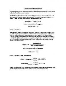
other inferential decisions typically employ confidence limits associated with α = 5%. Because inference analysis of relative error magnitudes is not necessarily a goal for which the assessment of relative error is undertaken, use of the simpler coefficient of variation statistic is preferred. Finally, the concept of precision is unfortunately counterintuitive. For example, if data exhibit higher precision (a desirable trait), the measure of precision is lower. This apparently contradictory feature of precision can lead to significant confusion. In contrast, although the concept of relative error is a negative trait (more error is not Fig. 1. Scatter plot of standard deviation plotted against mean concentration of Fe2O3 (wt.%) in desirable), if data exhibit higher reladuplicate analyses from a banded iron formation Fe ore deposit, illustrating the different absolute tive error, the measure of relative error and relative error results obtained by the various calculations described in the text. The incorrectly (the coefficient of variation) is higher determined average standard deviation (0.97 wt.%) is approximately 2/3 of the correctly deter(i.e., more nondesirable). Thus, unlike mined RMS standard deviation (1.49 wt.%). Sloping lines show the average duplicate coefficient of variation (dashed line), the RMS duplicate coefficient of variation (solid line), the average precision, the concept of relative error duplicate standard deviation divided by the average duplicate mean (dotted/dashed line), and the is consistent with its measurement, and RMS duplicate standard deviation divided by the average duplicate mean (dotted line). The averthus is an intuitively easier concept to age CV (6.84%) is approximately half the RMS CV (12.59%), and the average standard deviaunderstand and apply in error analysis. tion/average mean (4.61%) is approximately 2/3 of the RMS standard deviation/average mean We, therefore, believe that the coeffi(7.11%). m = slope. cient of variation should be used as a universal measurement of relative error in all geochemical ore deposit. This example demonstrates the important difapplications. ference between the average and RMS standard deviations, and illustrates how use of the average standard deviation Calculation of Relative Error underestimates (biases, in this case, by 35%) the error With the exception of the relative variance, the formuestimate (Stanley, 2006a; Stanley and Lawie, ????). The lae in Table 1 do not use the conventional formula for the four sloping lines that pass through the origin of Figure 1 mean to calculate the average relative error measure. This correspond to the relative errors determined by the four is because most of these measures use the standard deviapossible calculation strategies: (i) average duplicate cotion (or a proportional proxy for the standard deviation), efficient of variation (6.84% relative error; dashed line); which is not additive (Stanley, 2006a). As a result, a root (ii) RMS duplicate coefficient of variation (12.59% relamean square (RMS) calculation is undertaken to determine tive error; solid line); (iii) the average duplicate standard each of these average statistics (Stanley, 2006a; Stanley deviation divided by the average duplicate mean (4.61% and Lawie, ????). This calculation determines the average relative error; dotted/dashed line); and (iv) the RMS duplisquare and then takes the square root to determine the true cate standard deviation divided by the average duplicate average relative error measure. mean (7.11% relative error; dotted line). Note that these Unfortunately, two calculation approaches exist that last two relative error estimates pass through the intersecproduce different average relative error measures: (i) the tion points between the average replicate mean and avercoefficient of variation for each replicate set can be calcuage and RMS replicate standard deviations. Based on the lated and then the average (RMS) coefficient of variation above arguments, the RMS duplicate coefficient of variadetermined using the formula in Table 1; or (ii) the average tion (12.59%) represents the correct and unbiased estimate mean of the replicate sets can be divided into the average of relative error (Stanley, 2006a; Stanley and Lawie, ????). (RMS) standard deviation of the replicate sets. The former All other estimates are biased low, in some cases by as strategy produces the correct estimate of relative error. The much as 63%. latter is not really an average relative error; rather, it is a Comparing this correctly determined average coefficient ratio of the average replicate error divided by the average of variation with the results of a corresponding Thompsonreplicate mean, which is not the same thing. Examples of Howarth error analysis of these same data reveals several these two calculation strategies are presented in Figure 1. important points. Figure 2 presents a Thompson-Howarth In Figure 1, the vertical line defines the average duplierror analysis scatter plot of the duplicate data with a recate pair mean, and the two horizontal lines identify the gression model forced through the origin (and thus only inaverage and RMS standard deviations for a quality control volving a relative error term; i.e., a slope), using groups of data set of 100 Fe2O3 (wt.%) determinations of rotary drill 5 duplicate pair means and RMS standard deviations. The chip duplicate samples from a banded iron formation Fe slope derived from this analysis (3.62%) can be thought of



Average Relative Error in Geochemical Determinations • C.R. Stanley and D. Lawie

269

ical survey is 15%, then the expected measurement error in a sample with a Cu concentration of 220 ppm from that survey (but not necessarily one of the duplicates used to estimate this relative error) should not be estimated through simple multiplication of the concentration by the average relative error (i.e., 220 ppm × 0.15 = 33 ppm). This is because the relative error is an average of duplicate relative errors that exhibit a positively skewed distribution (Stanley, 2006a), and was calculated in a manner that is inconsistent with this predictive goal, using a method that does not minimize estimation error (i.e., a method such as least squares regression). Thus, it will not provide the Fig. 2. Thompson-Howarth error analysis scatter plot of the 100 duplicate Fe2O3 (wt.%) analyses best possible estimate of error. in Fig. 1. Diamonds represent original duplicate means and standard deviations; squares represent groups of 5 average means and RMS standard deviations (Stanley and Lawie, ????). Appropriate statistics that could be used to estimate the expected measas comparable with the RMS coefficient of variation for urement error in such a sample are the slope and intercept these data (12.59%). Unfortunately, the two estimates of of the regression line derived from a Thompson-Howarth relative error are significantly different (the Thompsonerror analysis (Thompson, 1973, 1982; Thompson and Howarth result is 71% lower than the RMS coefficient of Howarth, 1973, 1976, 1978; Howarth and Thompson, variation). 1976; Fletcher, 1981; Stanley and Sinclair, 1986; Garrett The observed discrepancies are an expected conand Grunsky, 2003; Stanley, 2003a,b). This is because sequence of these two error analysis approaches. The the regression used in Thompson-Howarth error analysis Thompson-Howarth error analysis result has been derived seeks to identify the expected value of the measurement from data plotted in a Cartesian coordinate system, because error at any concentration. It identifies a linear model that it estimates the absolute measurement error (the duplicate describes a “functional relationship” between concentrastandard deviation; the ordinate coordinate) at a given contion and error. Thus, if the slope and intercept derived from centration (the abscissa coordinate). In contrast, the RMS a Thompson-Howarth error analysis are 5% and 8 ppm, coefficient of variation effectively operates in a radial corespectively, then the best estimate of the standard deviaordinate system. The concentration of duplicate pairs is irtion of error in the sample with a concentration of 220 ppm relevant because the units of concentration (in this case, would be (220 ppm × 0.05) + 8 ppm = 19 ppm. This estiwt.%) cancel out in the formation of the coefficient of mate would involve the smallest estimation error because variation ratio. As a result, the individual coefficients of of the method used in its determination. variation describe slopes of lines from the origin to the Because the coefficient of variation is a descriptive duplicate pair points defined by their means and standard (structural relationship-type) measure of relative error, deviations. These slopes are functionally related to the raand because the squares of relative errors (the relative dial angles of a radial coordinate system. Thus, it should variances), like the squares of absolute errors (the varicome as no surprise that the RMS coefficient of variation ances), are additive (Francois-Bongarcon, 2005; Stanley and a Thompson-Howarth error analysis regression slope and Smee, 2005a,b, ????; Stanley, 2006b), relative errors produce significantly different results, precisely because of replicate measurements collected at various stages of the data are considered in completely different coordinate sample treatment can be used to determine the amount of systems. error introduced during each stage of sampling, preparation, and analysis of geochemical samples (Francois-BonAppropriate Use of the Average Relative Error garcon, 2005; Stanley and Smee, 2005a,b, ????). For example, because samples are collected in the field, crushed, The coefficient of variation is a descriptive estimate of subsampled, pulverized, subsampled again, and then anarelative error for a specific set of replicate measurements lyzed, sample replicates collected in the field will docu(the set used to make the estimate of relative error). Conment the total error introduced to the samples during this sequently, it describes a structural relationship between entire sampling/preparation/analysis protocol. In contrast, element concentration and measurement error. Thus, use sample replicates collected after crushing will document of the coefficient of variation should be restricted to those the amount of error introduced to the samples from that applications that are consistent with this characteristic. point onward in the sampling/preparation/analysis protoFor example, if the average relative error calculated (as col. If the sample replicates exhibit an average coefficient CV) from a set of duplicate determinations in a geochemof variation of 26%, whereas the post-crushing replicates

270

Exploration and Mining Geology, Vol. 16, Nos. 3–4, p. 265–274, 2007

exhibit an average coefficient of variation of 10%, then the coefficient of variation describing the magnitude of error introduced between initial sampling and subsampling after crushing (i.e., sampling error) is 24% (=  0.262 - 0.102 ). Use of relative errors in this application is appropriate because only descriptive measures of relative error are required for the decomposition of errors introduced during the sampling/preparation/analysis protocol. Relative errors can also be appropriately used to assess whether the data meet a required level of analytical quality, then the RMS coefficient of variation can be used for this purpose because it is a descriptive measure of analytical quality. For example, if 10% relative error is necessary to ensure the data collected are “fit for purpose” (Bettenay and Stanley, 2001), and a replicate data set exhibits 12% relative error, then one can conclude that this data set does not meet the required level of measurement precision to be used for the purpose it is intended. Although the slope and intercept derived from a Thompson-Howarth error analysis describe a functional relationship between concentration and measurement error, and thus can be used to predict the expected error in samples of known concentration, these parameters can also be used in the variance decomposition or “fit for purpose” applications described above. This is because, even though the parameters derived from a Thompson-Howarth error analysis are fundamentally and philosophically different from the structural coefficient of variation, they are derived from a regression, and thus can also be used to establish structural relationships in addition to functional relationships (Kendall and Stuart, 1966). Consequently, use of the parameters of a Thompson-Howarth error model can be used in both structural and functional relationship contexts, for prediction and description of the magnitude of measurement error.

The Importance of Large n

average relative error; Stanley, 2006a; Stanley and Lawie, ????) is presented in the Appendix. The standard error on the relative error (presented in relative terms) derived from Equation A7 in the Appendix is plotted as a function of the average relative error for different numbers of replicate determinations (p) in Figure 3. This illustrates that the standard error on the relative error is large for small numbers of replicate determinations. For example, for a single estimate of relative error of 15% determined from duplicates, the standard error on this estimate is 11% (a relative error of 73%; from Equation A7; Fig. 3). Analogously, Equation A11 can be used to determine the standard error on the average relative error of n replicate sets. For the duplicate data set presented in Figures 1 and 2, this standard error is 3.65% (on the estimate of 12.59%), and thus corresponds to a relative error of 29%. This relative error is large, in this case because n is relatively small (100). Thus, in order to obtain reasonably stable estimates of average relative errors, larger numbers of replicate sets (n) are commonly required. The poor precision exhibited by average relative errors is a consequence of the large scatter observed on plots of replicate mean versus replicate standard deviation (e.g., Fig. 1, 2), a feature resulting from the fact that duplicates provide poor estimates of both means and standard deviations. The functional form of Equation A11 also indicates that larger average relative errors will exhibit larger standard errors. Thus, a larger number of replicate determinations (p) will be required to obtain relatively accurate estimates of the average relative error, and the opposite will be true for small average relative errors. Consequently, the average relative error in a set of base metal assays, which typically exhibit relatively small average relative errors (such as 5%), can typically be determined reliably using smaller numbers of replicate sets (500 < n < 1000) than the average relative error in a set of gold assays, which typically exhibit relatively large average relative errors (such as 25%; Francois-Bongarcon, 2005; Stanley and Smee, 2005a,b, ????), which will require larger numbers of replicates (such as n > 2500).

The quality control duplicate data presented in Figures 1 and 2 exhibit significant scatter, and thus are similar to most duplicate quality control data observed in mineral exploration and mine assay data sets. The large scatter is a consequence of the very poor estimates of mean and standard deviation obtained from duplicate data. The magnitude of these estimation errors are defined by the standard errors on the duplicate means and standard deviations, and these are inverse functions of the square root of p, the number of replicates under consideration (in this case, p = 2; the relevant standard error formulae are presented in the Appendix). Because of the large scatter that occurs in duplicate quality control data sets, it is worth examining how this scatter affects the estimate of the average relative error. A derivation of the standard error on the average relative error (RMS coefficient of variation) of n replicate sets Fig. 3. Scatter plot of the standard error on the relative error (CV %; Equation A7) plotted against the relative error for different numbers of replicates (p). (effectively the estimation error of the



Average Relative Error in Geochemical Determinations • C.R. Stanley and D. Lawie

Conclusions Calculating relative errors in geochemical data sets is a task that has caused much confusion for geoscientists over the years because there are many ways to undertake such calculations. Fortunately, most of these approaches are numerically related to each other, and thus can be compared if appropriate steps are taken to convert these measures to a common standard. The coefficient of variation (one standard deviation divided by the mean) serves as this standard for a variety of reasons involving convention, theory, simplicity, generality, practicality, and philosophy. Use of the standard deviation is warranted over other statistics, precisely because it represents the standard measure of variation. Calculation of relative error should be undertaken using a root mean square approach because variances, and not standard deviations, are additive. Furthermore, to ensure an unbiased result, calculation of relative error should involve calculating the mean (RMS) of the individual estimates of relative error determined by each replicate set, rather than dividing the mean error by the mean concentration. Use of the coefficient of variation to describe relative error in a data set, calculated in the above manner, should be restricted to applications that require a bulk estimate of relative error in the data set under consideration. The relative error estimate should not be used to estimate the expected measurement error in individual samples. In contrast, results from Thompson and Howarth’s error analysis approach are suitable for the estimation of measurement error in individual samples, but not as a bulk description of relative error in the data set. Lastly, because of the large uncertainties associated with individual estimates of the coefficient of variation derived from duplicate samples, if an accurate average relative error estimate is desired, a very large number of duplicate samples must be used in the calculation (e.g., >500). Furthermore, if the expected relative error is large, an even larger duplicate data set (e.g., >2500) may be necessary.

Acknowledgments This research is motivated by the authors’ experiences witnessing the confusion brought about by the use of different measures of relative error by geologists and engineers at a number of mine sites. It was supported by a Natural Sciences and Engineering Research Council of Canada (NSERC) Discovery Grant, and a financial stipend and logistical support from CRC-LEME (Perth, Western Australia) to the first author.

References Bettenay, L., and Stanley, C.R., 2001, Geochemical data quality: The “fit-for-purpose” approach: Explore, Newsletter of the Association of Exploration Geochemists, v. 111, p. 12, 21–22. Fletcher, W.K., 1981, Analytical methods in geochemical

271

prospecting—Handbook of exploration geochemistry, 1: Amsterdam, Elsevier, 255 p. Francois-Bongarcon, D., 2005, Comment regarding “sample preparation of ‘nuggety’ samples: Dispelling some myths about sample size and sampling errors”: Explore, Newsletter of the Association of Applied Geochemists, v. 127, p. 17–18. Garrett, R.G., and Grunsky, E.C., 2003, S and R functions for the display of Thompson-Howarth plots: Computers and Geosciences, v. 29, p. 239–242. Howarth, R.J., and Thompson, M., 1976, Duplicate analysis in practice—Part 1: Examination of proposed methods and examples of its use: The Analyst, v. 101, p. 699–709. Kendall, M.G., and Stuart, A., 1966, The Advanced theory of statistics, 3: London, Griffin, 780 p. Long, S., 1998, Practical quality control procedures in mineral inventory estimation: Exploration and Mining Geology, v. 7, p. 117–127. Meyer, S.L., 1975, Data analysis for scientists and engineers: New York, Wiley, 513 p. Shaw, W.J., 1997, Validation of sampling and assaying quality for bankable feasibility studies [abs.]: Australian Institute of Mining and Metallurgy, The resource database towards 2000, Annual Meeting, May, Melbourne, Extended Abstracts, p. 41–49. Stanley, C.R., 1999, Treatment of geochemical data: Some pitfalls in graphical analysis: Association of Exploration Geochemists, 19th International Exploration Symposium, Vancouver, April, Quality Control in Mineral Exploration Short Course, p. 1–34. Stanley, C.R., 2003a, THPLOT.M: A MATLAB function to implement generalized Thompson-Howarth error analysis using replicate data: Computers and Geosciences, v. 29, p. 225–237. Stanley, C.R., 2003b, Corrigenda to “THPLOT.M: A MATLAB function to implement generalized Thompson-Howarth error analysis using replicate data.” [Computers and Geoscience, v. 29, p. 225–237]: Computers and Geosciences, v. 29, p. 1069. Stanley, C.R. 2006a, On the special application of Thompson-Howarth error analysis to geochemical variables exhibiting a nugget effect: Geochemistry: Exploration, Environment, Analysis, v. 6, p. 357–368. Stanley, C.R., 2006b, Numerical transformation of geochemical data, I: Maximizing geochemical contrast to facilitate information extraction and improve data presentation: Geochemistry: Exploration, Environment, Analysis, v. 6, p. 69–78. Stanley, C.R., and Lawie, D., ????, Thompson-Howarth error analysis: Unbiased alternatives to the large sample method for assessing non-normally distributed measurement error in geochemical samples: Geochemistry: Exploration, Environment, Analysis, v. ??, p. ???–???. Stanley, C.R., and Sinclair, A.J., 1986, Relative error analysis of replicate geochemical data: Advantages and applications [abs.]: GeoExpo, 1986: Exploration in the North American Cordillera, Association of Exploration Geochemists, Regional Symposium, Vancouver, Pro-

272

Exploration and Mining Geology, Vol. 16, Nos. 3–4, p. 265–274, 2007

grams and Abstracts, p. 77–78. Stanley, C.R., and Smee, B.W., 2005a, Sample preparation of ‘nuggety samples’: Dispelling some myths about sample size and sampling errors: EXPLORE, Newsletter of the Association of Applied Geochemists, p. 19–22. Stanley, C.R., and Smee, B.W., 2005b, Reply to comment by Francois-Bongarcon, D., regarding “sample preparation of ‘nuggety’ samples: Dispelling some myths about sample size and sampling errors”: EXPLORE, Newsletter of the Association of Applied Geochemists, p. 21–27. Stanley, C.R., and Smee, B.W., ????, Strategies for reducing sampling errors in exploration and resource definition drilling programs for gold deposits: Geochemistry: Exploration, Environment, Analysis, v. ??, p. ???–???. Thompson, M., 1973, DUPAN 3, A subroutine for the interpretation of duplicated data in geochemical analysis: Computers and Geosciences, v. 4, p. 333–340. Thompson, M., 1982, Regression methods and the comparison of accuracy: The Analyst, v. 107, p. 1169–1180. Thompson, M., and Howarth, R.J., 1973, The rapid estimation and control of precision by duplicate determinations: The Analyst, v. 98, p. 153–160. Thompson, M., and Howarth, R.J., 1976, Duplicate analysis in practice—Part 1. Theoretical approach and estimation of analytical reproducibility: The Analyst, v. 101, p. 690–698. Thompson, M., and Howarth, R.J., 1978, A new approach to the estimation of analytical precision: Journal of Geochemical Exploration, v. 9, p. 23–30. Appendix The following derivations determine the formulae of the standard error on the average coefficient of variation calculated from one set of p replicates, and from n sets of p replicates. The standard errors on the mean and standard deviation, for p replicates, are:

sm =

s p

, and ss =

s 2 ( p -1)

,

(A1)

A3 becomes:

s , (A2) m we can propagate standard errors on the mean and standard deviation through Equation A2 to determine the standard error on the relative error. This can be done using the error propagation equation:

2

æ dCV ö÷ çè ds ÷÷ø

2

s m + çç 2

i

æ dCV ö÷æ dCV ö ÷ s . (A4) ç çè dm ÷÷øçè ds ÷÷ø

ss + 2 çç 2

i

æ dCV ö÷ -s çç ÷= , and çè dm ÷÷ø m 2



æ -s ö÷ çè m ÷÷ø

sCV = çç



2

= CV

æ dCV ö÷ 1 çç ÷ = , èç ds ÷ø m

(A5)

2

2

2

æ s ö÷ æ 1 ö çç ÷ + çç ÷÷ çè p ÷ø çè m ÷ø

2

2

æ CV çç çè p

2

+

æ s ö÷ æ s çç ÷ + 2 ççè 2 ( p - 1)÷÷ø ççè m 2

2

ö÷æ 1 ö÷ ÷÷ççç ÷÷(0) (A6) øè m ø

ö÷ ÷÷ 2 ( p - 1) ÷ø 1

or:

CV 2 1 + . p 2 ( p -1)

sCV = CV

(A7)

Now, if we have several (i = 1 … n) estimates of the relative error from several sets of replicates, we can propagate the standard errors on these relative errors through the calculation of the average relative error to obtain an error on that estimate. Because errors are additive as variances, the average relative error must be calculated using a root mean square approach: n



mCV =

2

å CVi

i =1

n

.

(A8)

The error propagation formula for the variance on this average relative error is:

s

2 mCV

2 ææ ö ççç dmCV ö÷ 2 ÷÷ ÷÷ sCV ÷÷ , = å ççç i÷ i =1 ç çèçè dCVi ÷ø ÷ø n

(A9)

and the appropriate partial derivatives are:

æ dmCV çç ççè dCV

ö÷ 1 ÷÷ = ÷ 2 i ø

1 n

å CVi

2

æ 2CVi ö÷ çç ÷ èç n ÷ø

(A10)

i =1

p



n æ CVi ç 1 = ç n ççè m

CV

derived using a Taylor series expansion about the mean (Meyer, 1975; Stanley, 1990). In this application, Equation

ms

Making the appropriate substitutions, and assuming that the standard errors on the mean and standard deviation are independent, we obtain:

CV =

æ d y ö÷2 2 p -1 p æ d y öæ d y ö ÷÷ ç 2 s y = å ççç ÷÷ s xi + 2 å å ççç ÷÷÷çç ÷ s xi x j , (A3) ÷ ÷ ç ç ç i =1 è d xi ø i =1 j =i +1 è d xi øè d x j ÷ ÷ø

2

The required partial derivatives are:

respectively (Speigel, 1975). Given that the relative error (or coefficient of variation) is:

æ dCV ö÷ çè dm ÷÷ø

sCV = çç



ö÷ ÷÷ . ÷ø

Thus, the standard error on the average relative error is:





Average Relative Error in Geochemical Determinations • C.R. Stanley and D. Lawie

smCV =

2 æ ö 1 n ççæç CVi ö÷ 2 ÷÷ . ÷÷ sCV ÷÷ å çççç i÷ n i =1çèçè mCV ÷ø ÷ø

(A11)

The functional form of this equation dictates that as the number of relative error estimates (replicate sets, n) in-

273

creases, the standard error on the mean relative error will decrease. Additionally, because Equation A11 is a function of CVi, larger standard errors on the relative error will occur with larger relative errors. Curves defined by the standard error on the relative error for one replicate set with different numbers of replicate determinations (p = 2 through 10) are presented in Figure 3.

274

Exploration and Mining Geology, Vol. 16, Nos. 3–4, p. 265–274, 2007