Averaging models: parameters estimation with the R-Average ... - UV
Recommend Documents
Université Laval. Québec, Canada. Abstract. The holdout estimation of the expected loss of a model is biased and noisy. Yet, practicians often rely on it to select ...
lution that the obtained for the kernel ridge regression where now the noise variance term ... that not only a mean prediction is obtained for each sample but a full ...
8-24 µg/ml for ambroxol hydrochloride and levocetirizine dihydrochloride respectively. Results of the method were validated statistically and by recovery studies.
Dec 9, 2010 - CH NCH (curve discontinuity corresponds to the break in SOHO EIT observations). The ..... nomicheskii Zhurnal, 32(2), 165. Suzuki, T., Inutsuka ...
context of an averaging-type model for serial presentations (Anderson,. 1959); the ... of initial conditions and without using the method of sub-designs (Norman,. 1976 .... where s is the subjective evaluation of the attribute, b is the subject's bia
Abstractâ Method for geophysical parameter estimations with microwave radiometer data based on Simulated Annealing: SA is proposed. Geophysical ...
eno 1991; Kuhner and Felsenstein 1994; Yang et al. 1994). One particular aspect that ...... We thank Jeff Thorne and an anonymous referee for helpful comments ...
ESTIMATION OF PARAMETERS OF RCA. WITH EXPONENTIAL MARGINALS. Biljana Popovi c. Abstract. The estimation of parameters of time series whose ...
Dec 18, 1997 - maximum penalized likelihood approach and a Bayesian approach. .... used the EM algorithm for maximum penalized likelihood estimation.
This dissertation by Michael Peter Perrone is accepted in its ... Perrone, M. P. and L. N Cooper (1993) When Networks Disagree: Ensemble Method for Neural.
p x2 + 1xn?2dx(n ?1). S p n n. R1?n e. : For z < 1, we can bound this integral using. Z x=z x=0 p x2 + 1xn?2dx >. Z x=z x=0 xn?2 + (z)xndx; where (z) is de ned by.
estimation of unknown parameters in dynamic statistical models. It is a .... The optimization problems (2) or (3) are quadratic programming problems, involving a.
*Marco Del Negro: Federal Reserve Bank of Atlanta, 1000 Peachtree Street NE, Atlanta GA 30309-. 4470. .... to forecast US post-war inflation (N = 100, T = 480).
Abstract. Linear regression and regression tree models are among the most known regression models used in the machine learning community and recently ...
Jul 19, 2016 - The performance of both conventional ANNs and GANNs to estimate the stellar parameters as a ..... Java allows all performance tests to.
have in common the ability to work across sensory modalities (e.g., vision and audition) and to share ..... Shebo, 1982; Trick & Pylyshyn, 1993). EXPERIMENT 2: ...
based on original parametrization and on the logarithmic parametrization, results in parenthesis, for censored samples and fixed α = 2, β = 0.8 e λ = 0.1. Cens.
Frank Diebold, Cristian Huse, Dennis Kristensen, Oliver Linton, Nour Meddahi, Angelo Melino, Alex ... and Carrasco, Chernov, Florens and Ghysels (2004).
Arthur van Soest. DISCUSSION P. APER SERIES. Forschungsinstitut zur Zukunft der ...... 174 E. Fehr. J.-R. Tyran. Does Money Illusion Matter? An Experimental.
May 10, 2017 - dynamical systems conditioned on observations of the system. ... Markhov Chain Monte Carlo methods are commonly used to understand the ...
Feb 1, 2008 - In this paper we derive the consistency of the penalized likelihood ... Estimate, using maximum likelihood estimation (MLE) methods, the ...
require conditions that are generally not satisfied by models with simultaneity. ... where simultaneity is only one of many other possible features of the model.
COCOMO model. Index Terms--Software Cost Estimation, Uncertainty, Fuzzy. Numbers ... of different development modes and different application domains.
Second, the (unscaled) variance V of theorem 1 collapses to the variance of the estimator ..... wT making the CD-SNE asymptotically attain the Cramer-Rao lower bound. Precisely, let, ...... Dynamic Models, Oxford, Basil Blackwell. Gallant, A. R. ...
Averaging models: parameters estimation with the R-Average ... - UV
these models, proposed by Anderson (1981, 1982), identifies the averaging process as ... Furthermore, the method of sub-designs, proposed by Norman (1976) ... full three-way design (A Ã B Ã C) can be supplemented with three two-way. â.
Psicológica (2010), 31, 461-475.
Averaging models: parameters estimation with the R-Average procedure Vidotto G.∗ 1, Massidda D.1, and Noventa S.2 1
Department of General Psychology, University of Padova, Italy; 2 Department of Developmental ad Social Psychology, University of Padova, Italy
The Functional Measurement approach, proposed within the theoretical framework of Information Integration Theory (Anderson, 1981, 1982), can be a useful multi-attribute analysis tool. Compared to the majority of statistical models, the averaging model can account for interaction effects without adding complexity. The R-Average method (Vidotto & Vicentini, 2007) can be used to estimate the parameters of these models. By the use of multiple information criteria in the model selection procedure, R-Average allows for the identification of the best subset of parameters that account for the data. After a review of the general method, we present an implementation of the procedure in the framework of R-project, followed by some experiments using a Monte Carlo method.
Multi-attribute models generally follow three steps: evaluation of the attributes, integration of the obtained subjective dimensions, and a conclusive stage. In the last stage, the results of the previous processes are transformed into a ranking order, a set of pairwise preferences or a rating over some real interval (Lynch, 1985; Oral & Kettani, 1989). A subset of these models, proposed by Anderson (1981, 1982), identifies the averaging process as one of the widely used cognitive integration rules. The averaging process uses a weight and scale value parameters representation. Ratio scales are involved in the measurement of weights and equal-interval scales are used to measure values (Zalinski & Anderson, 1989). Furthermore, the method of sub-designs, proposed by Norman (1976) and Anderson (1982), allows for complete identifiability of these parameters by adjoining selected sub-designs to the full factorial design. For instance, a full three-way design (A × B × C) can be supplemented with three two-way ∗
Correspondence to: Giulio Vidotto; e-mail address: [email protected]. Acknowledgements: We would like to thank both the reviewers, for their appropriate and encouraging comments, and Cheng L. Qian, for the precious help he gave us.
G. Vidotto, et al.
462
sub-designs (A × B, A × C and B × C), and with three one-way sub-designs (A, B and C). In the current literature, this method is applied in different fields of Psychology, especially in Social (Falconi & Mullet, 2003; Girard, Mullet, & Callahan, 2002; Wang & Yang, 1998), Cognitive (Oliveira et al., 2006) and Developmental (Jäger & Wilkening, 2001) Psychology. A computer tool to cope with factorial design of Functional Measurement has recently been developed by Mairesse, Hofmans, and Theuns (2008). Despite the widespread use of the methodology, at present there are few tools for the estimation of averaging parameters. The first estimation procedure was developed by Zalinski (1984, 1986, 1987) and implemented in FORTRAN language. It had the capability to deal with the EAM (Equal Averaging Models) and the Complete DAM (Complete Differential Averaging Model) and to analyze the data from one subject and one session at a time. In addition, it did not account for information criteria (Wang & Yang, 1998). A second procedure has more recently been developed by Vidotto & Vicentini (2007) and focuses on the use of a different minimization algorithm for bounded parameters and on the introduction of an information criterion able to test several DAMs including the Complete DAM. The method has been implemented in the R-project environment: a modern, open-source and widely used framework for statistical analysis (R Development Core Team, 2009).
AVERAGI G MODELS Averaging models involve a two parameters representation: the scale value sjk, which represents the psychological scale value of the j-th level of an attribute k of some overt dimension, and the weight wjk, which represents its importance in the integrated response (Anderson, 1965). The averaging model represents the integrated response, R, as: ,
R=∑ i =0
wi si Ω
with
,
Ω = ∑i =0 wi
(1)
where the multi-index i = (j,k) accounts for the , overall number of attributes that are included in each stimuli set. Also, the condition i = 0 accounts for prior memorial information (it is also named the prior belief or initial state). Note that j = 1, ... Jk indexes the number of levels of a factor
Parameters estimation with R-Average
463
whereas k = 1, ... K indexes the factors of an experimental design. The relative weights of each stimulus thus depend on the other stimuli in the set. A factor k is said to be equally-weighted if wjk = wk for every j. Hence, the denominator of equation (1) has the same value in each cell of the design and can be absorbed into an arbitrary scale unit. If all the factors are equally-weighted, then the model is called an Equal-weight Averaging Model. However, accounting for crossover effects needs the introduction of different weight parameters that make the model more complex. These families of Differential-weight Averaging Models allow each stimulus (or group of stimuli) to have its own weight as well as its own scale value. The sum of the absolute weights in the denominator of equation (1) varies therefore from cell to cell in the design and the model becomes inherently non-linear. Nevertheless, this non-linearity generally introduces some analytical and statistical problems with regards to uniqueness, bias, convergence, reliability, and goodness of fit (Zalinski & Anderson, 1991).
R-AVERAGE – THE METHOD The R-Average method chooses the optimal model according to the “Ockham’s razor”: i.e. the one that fits empirical data by using the smallest set of weight parameters. Three goodness-of-fit indexes, based on Residual Sum of Squares (RSS) can be used to identify such a model: the adjusted Rsquare, the Akaike Information Criterion (AIC; Akaike, 1974, 1976), and the Bayesian Information Criterion (BIC; Schwarz, 1978; Raftery, 1995). Starting from the EAM as a baseline, one single weight parameter (or a set of them in the following steps) is changed and accepted (or rejected) for successive iteration on the result of a comparison between the baseline and the new model goodness of fit indexes (whenever ∆BIC < 2, difference in the AIC index is considered). The procedure iterates until no further improvements appear and represents a compromise between efficiency and performance. It has the capability of providing reliable estimation for each trial and for all the repeated measurements on a subject and can account for many repetitions to achieve reliable parameter estimation. The weight and scale value parameters are estimated by minimizing the RSS of the model. This is performed with the L-BFGS-B algorithm implemented by Byrd et al. (1995), which is an extension of the limited memory algorithm L-BFGS. Unlike the latter, the L-BFGS-B method is useful for solving large non-linear optimization problems with simple bounds on the variables. This algorithm does not require computation of second derivatives and the knowledge of the objective function structure.
G. Vidotto, et al.
464
The search direction employs a two-stage approach: the first stage identifies a set of active variables using the gradient projection method; in the second stage, a quadratic model is approximately minimized with respect to these free variables. Once a search direction is established, a line search is performed using a method described by Moré and Thuente (1990). If bounds are active, the algorithm stops when the norm of the projected gradient is sufficiently small. The choice of a method for solving constrained optimization problems stems on the Zalinski's (1987) recommendation that reliable estimations of weights can be provided when the minimization function is bounded, but other solutions, like Simulated Annealing methods, are also possible.
R-AVERAGE - THE IMPLEME TATIO The R-Average procedure has been implemented as a computerlibrary within the R-project (R Development Core Team, 2009). The RAverage library is well integrated in the R framework and it is specifically designed to easily manage data with several subjects and repeated experiments. The package, which includes R help pages and sample inputs, is available from the authors of this paper. For command-line beginners a practical graphical interface has been developed. The algorithm selects the combination of weights that shows the best fit indexes by considering each possible DAMs. It can be used for estimating weight and scale value parameters of a factorial design both for single subject, with repetitions, and for an entire sample; and summarize them into tables. It works on any number of factors and levels, and provides several ways to analyze data by handling the principal attributes of the functions that are listed below: •
• • •
Data: a matrix object containing the experimental data. The first column is filled with the initial state values whereas the others contain the sub-design response values (in order: one-way subdesigns, two-way sub-designs, etc.) and the full factorial design. If any sub-design is not available, the corresponding matrix columns must be loaded with ,A. Lev: a vector containing the number of the levels for each factor. Range: a vector containing the range of the scale responses R. Start: a vector containing the scale and the weight values indicating the starting point of the computational algorithm.
Parameters estimation with R-Average
• • •
• • •
• • •
465
Lower: a vector containing the lower bound of the scale and weight values. Upper: a vector containing the upper bound of the scale and weight values. All: a logical attribute that allows the procedure to test all the possible subset of DAMs with different weight parameters, or to restrict the analysis to a selected subset. Equal.weights: a numeric attribute that allows to fix the number of possible equal weights. Delta.weights: a numeric attribute that allows to choose a cut-off value at which different weights are considered equal. IC.diff: a vector containing the cut-off values for BIC and AIC at which different models with similar BIC/AIC are considered equivalent. Verbose: a logical attribute that allows to print general information on every step of the information criterion procedure. Maxit: the maximum number of minimization algorithm iterations, 55 for default. Method: the method followed by the algorithm for estimating the parameters. L-BFGS-B is the default option. However, due to the fact that results of R-Average implementation sometimes appear to be stuck in local minima (since they vary from the ideal values) a simulated annealing algorithm (option SANN) can be chosen. Nevertheless, its native implementation in the R framework (when called by the R-Average routine) has revealed to be time-consuming and require further analyses and adaptation. At present we highly discourage this option to be run.
MO TE CARLO SIMULATIO S EFFECTS OF PARAMETERS ORDER Starting from a strictly increasing monotonic factor A (with levels s1 < s2 < s3), five simulations were run using different permutations of A for the levels of factor B. The schema of the random synthetic data for each of the 1000 iterations is reported in Table 1.
466
G. Vidotto, et al.
Table 1. Schema of the random synthetic data for each iteration. Trend Factor A Factor B s1 s2 s3 s1 s2 s3 1 s1 s2 s3 s3 s2 s1 2 s1 s2 s3 s2 s1 s3 3 s2 s1 s3 s2 s1 s3 4 s2 s1 s3 s1 s2 s3 5 In every iteration a 5-row data matrix of random values was generated, followed by the addition of a normal N(0,1.5) distributed error, in order to calculate the responses Rjk. Results show that there are no effects in parameters estimation due to the factor's position in the algorithmic procedure or due to the monotonicity of the factors (R2 = 0.9778 for all trends). The scatter plot is reported in the left panel of Figure 1.
Figure 1. On the left: Estimated parameters versus theoretical parameters for Trend 1 to 5. On the right: Effects of the bounding on extreme value parameters (white: s1, light gray: s2, dark gray: s3). RELIABILITY OF THE PROCEDURE Synthetic responses Rjk for factorial design were calculated for a 3 × 3 experimental design. In the setting of Monte Carlo simulation were included different rows number (5,10,15) and different normal error (N(0,.5), N(0,1), N(0,1.5)) of the data matrix. These two attributes have
Parameters estimation with R-Average
467
been manipulated in order to simulate both different sets of measure repetitions and the influence of response variability on the data. In Table 3 the results of these Monte Carlo simulations are shown. The higher the number of rows, or the lower the standard deviation of the error, the better the estimation of the parameters is. In particular the procedure has good performance in recognizing the appropriate order of the parameters, as can be seen in Table 2. This fact is particularly important; in spite of the high variability that sometime affects the parameters estimation, at least the necessary condition of ordering is often fulfilled, ensuring a solid base for further improvement of the estimated values by means of iterative methods, R-Average attributes handling or other statistical methods. Table 2. umber of correctly estimated parameter order in the MCsimulations. wA2 < wB1 > wB2 < Scale Scale wA1 < Rows Error wA2 wA3 wB2 wB3 A B 0.5 1000 1000 1000 1000 1000 1000 5 1.0 985 993 954 909 979 863 1.5 873 942 835 793 820 637 0.5 1000 1000 1000 1000 1000 1000 10 1.0 1000 999 994 983 999 977 1.5 980 986 955 890 966 845 0.5 1000 1000 1000 1000 1000 1000 15 1.0 1000 1000 999 996 1000 995 1.5 995 996 982 937 991 919 Results, however, deserve different considerations depending on the type of estimated parameters: s-type parameters follow a normal distribution centered on the true value of the parameter and with a standard deviation that increases with the error standard deviation, but decreases with the larger sets of available data. Also, s-parameters that are closer to the bounding value (0-20) are generally estimated with an asymmetric distribution as can be inferred by the right panel of Figure 1. In contrast, w-type parameters do not follow a normal distribution. In Table 3 the ratios of the w-parameters are reported, since their proportions are more important then their values.
Table 3. Results of Monte Carlo simulations. Estimated parameters are reported for each condition on the number of Rows of the data matrix and on the normal Error that was added to synthetic data. Each condition contains the mean estimated parameter and (between brackets) the interval that contains the 95% of the values estimated during the Monte Carlo study. For the scale value s parameters the mean value coincide with 1.96s, where s is the standard deviation of the normal distribution of s.
468 G. Vidotto, et al.
Parameters estimation with R-Average
469
It can be seen that exact estimation of the real value of the w-ratios are less precise than those of s-parameters; in particular, a higher error standard deviation increases the difficulty in estimating the exact value. Nevertheless, as we noticed before, more reliable values of the ratios can always be searched if the fundamental requirement of ordering is fulfilled. EFFECTS OF ATTRIBUTES HA DLI G Monte Carlo simulations have been run to test the procedure improvement in parameters estimation with different settings of the algorithmic attributes. Five different attributes have been handled in the simulation for the conditions of “5 rows, 1.5 variance” and “10 rows, 1.0 variance”; the first condition was chosen to reproduce an experiment with a low number of trials and an high variance in data, the second condition to reproduce an experimental situation with a good control in data variance and an adequate number of trials. Results are described below and summarized in Tables 4, 5 and 6. •
•
•
•
Changes of bounds or lower and upper attributes: results show that changing the range of the weights parameters does not affect the reliability of the procedure since the algorithm is based on the conservation of the ratios between w-parameters. The scale for wparameters can thus be chosen according to the experimental setting. Attribute equal.weights set equal to 2: results show that equating a priori a couple of parameters could improve estimation reliability (see in Tables 4, 5 and 6). Attribute delta.weights set equal to 0.5: results show that setting the criterion value to 0.5 at which two weights are considered equal makes order recognition more stable (as can be seen in Table 4) but worsen the mean estimated parameters value in presence of high data variability (5-1.5 simulation, Table 5); instead, in the presence of contained variability the results are improved (10-1.0 simulation, Table 6). Attributes IC.diff set to 1: using a restrictive acceptance criterion for BIC selection slightly worsens the reliability of the procedure in the presence of larger variance. Reliability of the order of the parameters of factor B is improved, yet the reliability of the scale order of the other parameters is reduced. Notice that the change in IC.diff does not affect mean estimated parameters as can be seen in Tables 5 and 6.
G. Vidotto, et al.
470
•
•
Attributes All set to True: allowing the algorithm to span all the possible DAMs can increase the reliability of the procedure. Results show that there is a strong improvement both in the exact estimation of parameters (Tables 5 and 6) and in the recognition of the correct parameters order, as can be seen in Table 4. Combination of All equal to True and delta.weights equal to 0.5: performance can than be strongly improved by combining the best previous attribute manipulations as in Table 4, 5 and 6.
Table 4: Results of Monte Carlo simulations for different attributes manipulation conditions. 5 Rows 1.5 Error Default Equal.weights=2 Delta.weights=0.5 IC.diff=1 All=True All=TRUE and delta.weights=0.5 10 rows 1.0 error Default Equal.weights=2 Delta.weights=0.5 IC.diff=1 All=True All=TRUE and delta.weights=0.5
Table 6. Results of Monte Carlo simulations for different attributes manipulation conditions on the case of 10 rows and 1.0 error variance.
472 G. Vidotto, et al.
Parameters estimation with R-Average
473
GE ERAL DISCUSSIO R-Average consists of a general procedure and an R-library for parameter estimation and model selection of the averaging model. It is well integrated in the R framework (R Development Core Team, 2009). The procedure, based on the “Ockham’s Razor” and on the bounded minimization algorithm L-BFGS-B, provides good estimates of the parameters of the averaging models and several goodness-of-fit indexes useful for model comparison. It also allows the management of several repetitions both for single subject and for group data and to estimate parameters for incomplete factorial designs. In addition, it provides several attributes useful to improve analysis: for instance, the number of equal weights can be established a priori and several criteria can be set to adapt the procedure flow to the experimental needs. These attributes are listed previously in this text. Results of Monte Carlo simulations show good reliability of the procedure in parameters estimation and excellent reliability in recognition of the parameters importance order. This latter result ensures good behavior of the procedure and implies that more accurate estimations of the parameters could be obtained. For this purpose, further developments of the procedure will allow the selection and fixing of the parameter values. Then a Monte Carlo simulation study can be conducted based on experimental data, in order to obtain more reliable parameters estimation. Finally, since reliability reduces with the increase of data variability, one remaining issue concerns the theoretical validity of group analyses: this issue was previously raised by Zalinski and Anderson (1991) because these analyses can cause bias in the estimated weights and scale values; nevertheless, if the variability of the responses is not extreme, the RAverage procedure can be carefully used even for group data.
REFERE CES Akaike, H. (1974). A new look at the statistical model identification. IEEE Transactions on Automatic Control, 19 (6): 716–723. Akaike, H. (1976). Canonical correlation analysis of time series and the use of an information criterion. In R. K. Mehra & D. G. Lainotis (Eds.), System identification: Advances and case studies (pp. 52–107). New York: Academic Press. Anderson, N. H. (1965). Averaging versus adding as a stimulus combination rule in impression formation. Journal of Experimental Psychology, 70, 394-400. Anderson, N. H. (1981). Foundations of Information Integration Theory. New York: Academic Press. Anderson, N. H. (1982). Methods of Information Integration Theory. New York: Academic Press.
474
G. Vidotto, et al.
Byrd, R. H., Lu, P., Nocedal, J., & Zhu, C. (1995). A limited memory algorithm for bound constrained optimization. Journal Scientific Computing, 16, 1190–1208. Falconi, A., & Mullet, E. (2003). Cognitive algebra of love through the adult live. International Journal of Aging and Human Development, 57 (3), 275–290. Girard, M., Mullet, E., & Callahan, S. (2002). Mathematics of forgiveness. The American Journal of Psychology, 115 (3), 351–375. Jäger, S., & Wilkening, F. (2001). Development of Cognitive Averaging: When Light and Light Make Dark. Journal of Experimental Child Psychology, 79, 323–345. Lynch, J. G., Jr. (1985). Uniqueness issues in the decompositional modeling of multiattribute overall evaluations: an information integration perspective. Journal of Marketing Research, vol. 22 (1), pp. 1-19. Mairesse, O. , Hofmans, J. & Theuns, P. (2008). The Functional Measurement Experiment Builder Suite: Two JAVAbased programs to generate and run Functional Measurement experiments. Behavior Research Method, 38, 692-697. Moré, J.J. & Thuente, D.J. (1990). On-line search algorithms with guaranteed sufficient decrease. Mathematics and Computer Science Division Preprint MCS-P153-0590, Argonne National Laboratory (Argonne, IL). Norman, K. L. (1976). A solution for weights and scale values in functional measurement. Psychological Review, 83 (1), 80-84. Oliveira, A. M., Teixeira, M. P., Fonseca, I. B., Santos, E. R., Oliveira, M. (2006). Interemotional comparisons of facially expressed emotion intensities: Dynamic ranges and general-purpose rules. In Kornbrot, D.E., Msefti, R.M., & MacRae, A.W. (Eds). Fechner Day 2006. Proceedings of the 22nd Annual Meeting of the International Society for Psychophysics (pp. 239-244). St. Albans UK: The International Society for Psychophysics. Oral, M. & Kettani, O. (1989). Modelling the process of multiattribute choice. The Journal of the Operational Research Society, vol. 40 (3), pp. 281-291 R Development Core Team. (2009). R: A language and environment for statistical computing. Vienna, Austria. Raftery, A. E. (1995). Bayesian model selection in social research. Sociological Methodology, 25, 111–163. Schwarz, G., 1978 Estimating the dimension of a model. The Annals if Statistics, 6 (2), 461–464. Vidotto, G. & Vicentini, M. (2007). A general method for parameter estimation of averaging models. Teorie e modelli, 12 (1-2), 211-221. Wang, M., & Yang, J. (1998). A multi-criterion experimental comparison of three multiattribute weight measurement methods. Journal of Multicriteria Decision Analysis, 7, 340–350. Zalinski, J. (1984). Parameter estimation: An estimated variance-covariance matrix for averaging model parameters in information integration theory. Behavior Research Methods, Instruments, & Computer, 16 (6), 557-558. Zalinski, J. (1987). Parameter estimation for the averaging model of information integration theory. Unpublished doctoral dissertation, University of California, San Diego, La Jolla, CA. Zalinski, J., & Anderson, N. H. (1986). Average: a user-friendly fortran-77 program for parameter estimation for the averaging model of information integration theory [computer software]. San Diego, CA.
Parameters estimation with R-Average
475
Zalinski, J., & Anderson, N. H. (1989). Measurement of importance in multi-attribute models. In J. B. Sidowski (Ed.), Conditioning, cognition and methodology. Contemporary issues in experimental psychology (pp. 177–215). Lanham, MD: University press of America. Zalinski, J., & Anderson, N. H. (1991). Parameter estimation for averaging theory. In N. H. Anderson (Ed.), Contributions to Information Integration Theory (Vol. 1: Cognition, pp. 353–394). Hillsdale, NJ: Lawrence Erlbaum Associates. (Manuscript received: 15 June 2009; accepted: 5 November 2009)