Additional Key Words and Phrases: Test case generation; Boundary Value Analysis; coincidental correctness; domain faults. 1. INTRODUCTION. Testing is an ...
Avoiding Coincidental Correctness in Boundary Value Analysis R. M. Hierons School of Information Systems, Computing, and Mathematics Brunel University, UK In partition analysis we divide the input domain to form subdomains on which the system’s behaviour should be uniform. Boundary value analysis produces test inputs near each subdomain’s boundaries to find failures caused by the boundaries being incorrectly implemented. However, boundary value analysis can be adversely affected by coincidental correctness — the system produces the expected output for the wrong reason. This paper shows how boundary value analysis can be adapted in order to reduce the opportunity for coincidental correctness. The main contribution is to automated test data generation in which one cannot rely on the expertise of a tester. Categories and Subject Descriptors: D2.4 [Software Engineering]: Software/Program Verification; D2.5 [Software Engineering]: Testing and Debugging General Terms: Reliability, Theory, Verification Additional Key Words and Phrases: Test case generation; Boundary Value Analysis; coincidental correctness; domain faults
1. INTRODUCTION Testing is an expensive part of the software development process, often consisting of in the order of fifty percent of the overall budget. Testing also fails to find many of the existing problems in software. Testing is thus a difficult and expensive process and the development of efficient effective test techniques is a major research topic. Most testing techniques can be categorized as either black-box (they are based on the specification) or white-box (they are based on the code). Black-box and white-box techniques complement and typically are applied in different phases of the testing process. Partition Analysis and Boundary Value Analysis are two of the most popular black-box testing techniques. In Partition Analysis (PA) [Clarke et al. 1982; Goodenough and Gerhart 1975; Jeng and Forgacs 1999; Jeng and Weyuker 1994; Ostrand and Balcer 1988; Richardson and Clarke 1985; White and Cohen 1980] we divide (partition) the system’s input domain D into a finite set of subdomains S1 , . . . , Sn such that, according to the specification, the system’s behaviour should be uniform on each Si . The idea R. M. Hierons, School of Information Systems, Computing, and Mathematics, Brunel University, Uxbridge, Middlesex, UB8 3PH, United Kingdom. Permission to make digital/hard copy of all or part of this material without fee for personal or classroom use provided that the copies are not made or distributed for profit or commercial advantage, the ACM copyright/server notice, the title of the publication, and its date appear, and notice is given that copying is by permission of the ACM, Inc. To copy otherwise, to republish, to post on servers, or to redistribute to lists requires prior specific permission and/or a fee. c 20YY ACM 0000-0000/20YY/0000-0001 $5.00 ° ACM Journal Name, Vol. V, No. N, Month 20YY, Pages 1–0??.
2
·
is that if the system’s functionality on a subdomain Si is wrong then it is likely to fail on most values from Si and so it is sufficient to take a few test inputs from each subdomain. The partition could result from analysis carried out by the tester [Grochtmann and Grimm 1993; Ostrand and Balcer 1988] or from an automated approach based on a formal specification or model (see, for example, [Amla and Ammann 1992; Dick and Faivre 1993; Hierons 1997; Horcher and Peleska 1995; Offutt and Liu 1999; Stocks and Carrington 1996]). However, it has been observed that such test inputs are unlikely to find failures caused by the boundaries of the subdomains being incorrect. In Boundary Value Analysis (BVA) we thus produce test inputs close to the boundaries of the subdomains with the aim of finding shifts in boundaries (see, for example, [Clarke et al. 1982; Jeng and Forgacs 1999; Jeng and Weyuker 1994; White and Cohen 1980]). The essential idea behind BVA is that, if a boundary in the code is wrong, then some input values will have the wrong functionality applied to them and this will include values near to the expected boundary. By choosing test inputs near to the boundaries in the specification, and on either side of each boundary, we are likely to find any boundary shifts. However, coincidental correctness can affect this: the wrong functionality could be applied without leading to the wrong output. Little attention has been paid to the problem of finding test inputs, for BVA, that do not suffer from coincidental correctness. Instead, most work on BVA has used geometric arguments to drive the generation of a test suite with the property that if there is a boundary shift then it is likely that at least one test input will be in the wrong subdomain. Clarke et al. [Clarke et al. 1982], when considering the use of BVA for path testing, do observe that the tester might note the problem of coincidental correctness and generate additional tests. The work described in this paper could be seen as a formalization and generalization of the suggestions found in [Clarke et al. 1982]. The observations made are particularly relevant to the area of automated test data generation since here we cannot rely on an experienced tester avoiding the types of coincidental correctness identified in this paper. This paper shows that if we only apply a geometric approach to the generation of test input for BVA then it is possible for us to generate test input that cannot detect boundary shifts. We call this predictable coincidental correctness and focus on the problem of generating test inputs, for BVA, that do not suffer from this problem. We start with the case usually considered in the literature on BVA, where the specification is deterministic. We demonstrate that predictable coincidental correctness can occur here and also that the natural approach to solving this problem is not always sufficient. While many systems and specifications are deterministic, non-determinism can occur in a specification as a result of abstraction and may appear in both a specification and implementation when considering distributed systems. We thus also consider the case where the specification, and possibly the implementation, is non-deterministic. This analysis leads to the suggestion that adaptive test input generation techniques could be used when applying BVA with non-deterministic specifications. In this paper we define properties that test cases used in BVA should have but this leads naturally to approaches for generating such test cases: test case generation can be seen as a problem of searching for test cases that satisfy these properties. ACM Journal Name, Vol. V, No. N, Month 20YY.
·
3
Test case generation may thus be driven by automated search techniques. As noted earlier, it appears likely that the results and ideas outlined in this paper will be most relevant to automated test generation. This paper has the following structure. Section 2 describes PA and BVA. Section 3 shows how we can demonstrate that some test inputs are incapable of finding boundary shifts and thus should be avoided in BVA. On this basis BVA is adapted to avoid such values. Section 4 extends this, showing that sometimes additional factors must be considered. Section 5 then considers the use of BVA when testing from a non-deterministic specification. Finally, Section 6 draws conclusions. 2. PARTITION ANALYSIS AND BOUNDARY VALUE ANALYSIS 2.1 Overview PA and BVA are two related black-box testing techniques in which we partition the input domain D into a set of subdomains S1 , . . . , Sn and generate test inputs on the basis of this. The subdomains are chosen so that, according to the specification, the behaviour should be uniform on each Si . Throughout this paper we assume that such a partition is being used as the basis of test generation and fi denotes the specified functionality on subdomain Si (1 ≤ i ≤ n). PA and BVA have been justified in terms of the following two types of faults. (1) Computation faults: the wrong function is applied to some subdomain Si in the implementation. (2) Domain faults: the boundary between two subdomains in the implementation is wrong. In PA we produce test inputs that aim to find computation faults. Since a computation fault leads to the wrong function being applied throughout some subdomain Si , in PA it is normal to choose just a few test inputs from each subdomain (or even just one). BVA aims to find domain faults by using test inputs near to the boundaries. Let us suppose that the boundary between adjacent subdomains Si and Sj is incorrectly implemented leading to subdomains Ai and Aj . Then a test input x will have the wrong functionality applied to it, and thus is capable of detecting this fault, if x is in the wrong subdomain in the implementation: either x ∈ Si and x 6∈ Ai or x ∈ Sj and x 6∈ Aj . Approaches to BVA thus aim to produce a set of test inputs such that, if there is a domain fault, then it is likely that at least one of the test inputs will be in the wrong subdomain in the implementation. The essential idea is illustrated in Figure 1. BVA can be seen as an approach that assumes that the input domain of the implementation can be partitioned to form some {A1 , . . . , An } such that for all 1 ≤ i ≤ n, Ai is ‘similar to’ Si , the behaviour of the implementation is uniform on each Ai , and the function f¯i defined by the implementation on Ai conforms to fi (if f¯i does not conform to fi then we expect PA to have found this computation fault). Thus, for each (Si , fi ) we have a corresponding (Ai , f¯i ). The test inputs generated in BVA target the types of faults allowed by these assumptions — domain faults. Throughout this paper we assume that for each (Si , fi ) there is such a (Ai , f¯i ). ACM Journal Name, Vol. V, No. N, Month 20YY.
4
· test input in correct subdomain expected boundary
test input in wrong subdomain actual boundary Fig. 1.
Test inputs for BVA
a pair that is capable of finding the domain fault a pair that is not capable of finding the domain fault expected boundary actual boundary
Fig. 2.
Using more than one pair of test inputs for BVA
There are several approaches to BVA (see, for example, [Jeng and Forgacs 1999; Jeng and Weyuker 1994; Richardson and Clarke 1985; White and Cohen 1980]). These are based on geometric arguments in which we choose a set T of test inputs for a boundary B such that if there is a boundary shift in B within the implementation then it is likely that at least one value from T will be in the wrong subdomain in the implementation. In order to simplify the explanation in this paper we assume that the approach used is to generate pairs of test inputs around the boundaries — the essential idea extends to the other approaches to BVA. Consider a boundary B between subdomains Si and Sj from the specification. Suppose that the values on the boundary are in Si . In order to check the boundary B we produce pairs of test inputs of the form (x, x0 ) such that x is on the boundary (and thus in Si ) and x0 is in Sj and is close to x. If x and x0 are in the correct subdomains Ai and Aj of the implementation then the actual boundary must pass between x and x0 . If neither subdomain contains the boundary then we produce pairs of test inputs with one on either side of the boundary. Often we produce more than one such pair for a boundary, ideally spread out over the boundary. Figure 2 illustrates this idea. 2.2 BVA: the scope for coincidental correctness Let us suppose that in the (deterministic) specification there are two adjacent subdomains Si and Sj on which the system’s functionality should be fi and fj respectively. Further suppose that the boundary between subdomains Si and Sj is ACM Journal Name, Vol. V, No. N, Month 20YY.
·
5
incorrectly implemented leading to subdomains Ai and Aj in the implementation and that we use a test input x with x ∈ Si and x ∈ Aj . Thus, x is in the wrong subdomain in the implementation. However, x will only detect this domain fault if a failure is observed and this will only happen if fi and fj produce different output on x. Thus, if fi (x) = fj (x) then the test input x cannot detect a domain fault in which x lies in Aj rather than Ai . If this is the case then x is a poor choice of test input, for checking the boundary between Si and Sj , irrespective of whether it is on the boundary or, if it is not on the boundary, how close it is to the boundary. Thus, assuming that the specification and implementation are deterministic we get the following notion of coincidental correctness. Definition 1. For boundary value analysis, coincidental correctness occurs for input x if x ∈ Si and x ∈ Aj for some i 6= j but fi (x) = f¯j (x). Assuming that there are no computation faults, the final part of the condition reduces to fi (x) = fj (x). From the above it is clear that the choice of test input for BVA should not be based solely on geometric arguments — it should also consider the functions expected in the different subdomains. The following sections consider ways of avoiding such problems and separately investigate two cases: where the specification is deterministic and where it is non-deterministic. 3. USING DISTINGUISHING TEST INPUT FOR DETERMINISTIC SYSTEMS This section shows how we can eliminate a potential source of coincidental correctness in BVA when testing from a deterministic specification. Throughout this section we assume that the input domain D has been partitioned1 to form subdomains S1 , . . . , Sn and, since this is a partition, the Si are pairwise disjoint and cover D. When applying BVA to check the boundary between adjacent subdomains Si and Sj we produce pairs of test input (x, x0 ) such that: (1) x ∈ Si ; (2) x0 ∈ Sj ; and (3) x and x0 are close together. If possible, we choose one of x and x0 to be on the boundary between Si and Sj . Note that the third point requires us to have at least an ordering on the input values and ideally a metric; without this we have no notion of a boundary and so cannot apply BVA. It is relatively straightforward to define a notion of ‘close’ for numbers or tuples of numbers. It is less clear for other datatypes such as strings, although there are a number of metrics such as the Hamming distance. Even with numbers, there are alternative notions of ‘close’; for some examples a distance of 1 would be close while for others we might require a much smaller distance such as 10−5 and thus the definition could rely on the tester’s domain knowledge. In test generation we can replace ‘close’ by ‘as close as possible’ and see this as an 1 Overlapping
subdomains may occur in some subdomain based test techniques, but typically these are white-box techniques. By contrast, black-box subdomain techniques usually produce true partitions of the input domain. ACM Journal Name, Vol. V, No. N, Month 20YY.
6
·
optimization problem; we want an adequate pair of test inputs with minimum distance between them. Example 1. We are using BVA to test from the following specification of a simple system that determines the amount charged to a customer for buying w units of water and e units of electricity in a given month, where w and e are non-negative real numbers. The basic charge for a unit of water is c1 and the basic charge for a unit of electricity is c2 and thus if there are no discounts then the overall charge to the customer is c1 w + c2 e. However, if the customer has purchased at least b units of water in the month (w ≥ b) then there is a 20% discount on the electricity. Thus, the specification contains two cases: (1 ) Subdomain S1 = {(w, e) ∈ R × R|0 ≤ w < b ∧ e ≥ 0} and corresponding function f1 (w, e) = c1 w + c2 e. (2 ) Subdomain S2 = {(w, e) ∈ R × R|w ≥ b ∧ e ≥ 0} and corresponding function f2 (w, e) = c1 w + 0.8c2 e. We have one boundary at w = b. Suppose that in BVA we use a test case (b, 0) and that in the implementation the subdomains are A1 = {(w, e) ∈ R × R|0 ≤ w < b + ∆ ∧ e ≥ 0} and A2 = {(w, e) ∈ R × R|w ≥ b + ∆ ∧ e ≥ 0} respectively for some ∆ > 0. While our test case is in the wrong subdomain in the implementation this does not lead to a failure since f1 (b, 0) = c1 b = f2 (b, 0). Thus, due to coincidental correctness, the value (b, 0) fails to find this boundary shift even though it is in the wrong subdomain in the implementation. Note that any such boundary shift of size ∆ for ∆ > 0 will go undetected: we fail to detect arbitrarily large boundary shifts. This example shows that if we make an inappropriate choice of test input then coincidental correctness can lead to arbitrarily large boundary shifts going undetected. Further, it shows that there are cases where standard approaches to BVA leads to test input with the property that we can know in advance that such boundary shifts will go undetected. The failure to find the boundary shift was due to coincidental correctness. However, it is an example of predictable coincidental correctness. We wish to avoid such situations and the following definition captures the property we require. Definition 2. Let us suppose that we have adjacent subdomains Si and Sj . Then test input x is a distinguishing test input for (Si , Sj ) if and only if x ∈ Si and fi (x) 6= fj (x). The important point here is that if x ∈ Si is not a distinguishing test for (Si , Sj ) then it cannot detect a shift in the boundary between Si and Sj . In such a case we should not use x, in BVA, to check the boundary between Si and Sj . Definition 3. Let us suppose that we have adjacent subdomains Si and Sj , test input x ∈ Si , and test input x0 ∈ Sj . Then (x, x0 ) is distinguishing for (Si , Sj ) if x is a distinguishing test input for (Si , Sj ) and x0 is a distinguishing test input for (Sj , Si ). In BVA, when producing test input to check the boundary between adjacent subdomains Si and Sj we should produce pairs of test input of the form (x, x0 ) such that: ACM Journal Name, Vol. V, No. N, Month 20YY.
·
7
(1) (x, x0 ) is distinguishing for (Si , Sj ); and (2) x and x0 are close together. Naturally, the conditions we require for ‘close together’ to make sense are equivalent to those required for us to be able to apply BVA and so the above is relevant whenever we can use BVA. Note that conceptually the observation that we require distinguishing tests is related to work on testing from boolean specifications (see, for example, [Kuhn 1999; Tsuchiya and Kikuno 2002]). In this previous work, for a hypothesized fault we can determine the condition placed on the input in order to detect the fault. We now show how test input generation, for BVA, can be driven by these observations. Example 2. Consider Example 1. The specification contains two cases: (1 ) Subdomain S1 = {(w, e) ∈ R × R|0 ≤ w < b ∧ e ≥ 0} and corresponding function f1 (w, e) = c1 w + c2 e. (2 ) Subdomain S2 = {(w, e) ∈ R × R|w ≥ b ∧ e ≥ 0} and corresponding function f2 (w, e) = c1 w + 0.8c2 e. We can generate a pair (x, x0 ) that is distinguishing in the following way. Let x = (w, e) and x0 = (w0 , e0 ). Since the boundary is w = b it is natural to fix e = e0 . We can also insist that the two points are ² apart for some small ² > 0 and without loss of generalization we assume that w0 > w. Thus, our two points are x = (w, e) and x0 = (w + ², e) for w < b and w + ² ≥ b. We now want to have f1 (x) 6= f2 (x) and f1 (x0 ) 6= f2 (x0 ). This reduces to c1 w + c2 e 6= c1 w + 0.8c2 e and c1 (w +²)+c2 e 6= c1 (w +²)+0.8c2 e with two variables w and e. Both of these simply reduce to e 6= 0. We might thus produce pairs of test input such as x1 = (b − ², L) (in S1 ) and x01 = (b, L) for some large L and x2 = (b − ², 0.01) and x02 = (b, 0.01). In this example test data generation was simplified by assuming that e0 = e and w = w + ². However, automated test data generation is possible without this simplification since the constraints are still linear without these assumptions (assuming we use the metric that the distance between x and x0 is |w − w0 | + |e − e0 |) and thus the problem of automated test data generation is a linear programming problem and so can be solved using standard algorithms. If the constraints/boundaries are not linear, it may still be possible to automatically generate test data using more general search and constraint solving algorithms. We have seen that in choosing test input for BVA, in order to check the boundary between Si and Sj , we should use test inputs that are distinguishing for (Si , Sj ) or distinguishing for (Sj , Si ). We now show that this is not always sufficient. 0
4. USING ROBUST TEST INPUT FOR DETERMINISTIC SYSTEMS The previous section showed how we can produce test inputs, for BVA, that avoid a form of predictable coincidental correctness. However, the example considered used real-value functions and in analyzing these we ignored a potentially important issue: the functions will not be implemented using reals. This section shows that the approximation to the reals, used in the implementation, can be factored into our choice of test input for BVA. ACM Journal Name, Vol. V, No. N, Month 20YY.
8
·
Throughout this section we assume that an implementation uses floating point numbers such that: (1) A real x is represented by a value, formed by truncating x, denoted truncate(x) and this gives precision δ; and (2) There is a value M AX > 0 such that the floating point values are all less than M AX and greater than or equal to −M AX. Based on this, we can map a real value x onto a floating point value t(x) that approximates it. The following is one way of achieving this. Definition 4. Given a real number x let reduce(x) denote the real number that is less than M AX and greater than equal to −M AX and may be obtained from x by repeated addition or subtraction of 2M AX. Then t(x) = reduce(truncate(x)). We can also define an equivalence relation ≡ on the reals, such that x ≡ y if and only if they are represented by the same floating point value. Thus x ≡ y if and only if t(x) = t(y). If x ≡ y does not hold then we write x 6≡ y. We need to consider what we mean by a floating point valued program correctly implementing a real valued specification. The following is a simple notion of correctness of the function fp defined by our program p relative to the function fs defined by our specification2 . Definition 5. Let us suppose that x is an input, yp = fp (x), and ys = fs (x). Then p is correct on input x if and only if yp = t(ys ). Program p is correct if and only if p is correct on all input. Throughout this paper F denotes the set of floating point numbers used. We are now ready to consider the problem of generating test input for BVA. Definition 6. Let us suppose that we have adjacent subdomains Si and Sj and a test input x that has been introduced to detect shifts in the boundary between Si and Sj . Then x is a strongly distinguishing test input for (Si , Sj ) if and only if x ∈ Si and fi (x) 6≡ fj (x). Definition 7. Let us suppose that we have adjacent subdomains Si and Sj , test input x ∈ Si , and test input x0 ∈ Sj . Then (x, x0 ) is strongly distinguishing for (Si , Sj ) if x is a strongly distinguishing test input for (Si , Sj ) and x0 is a strongly distinguishing test input for (Sj , Si ). Thus in BVA, when producing pairs of test input to check the boundary between adjacent subdomains Si and Sj for real-valued functions we should produce pairs of the form (x, x0 ) such that: (1) (x, x0 ) is strongly distinguishing for (Si , Sj ); and (2) x and x0 are close together. 2 There
are alternative ways of defining correctness, such as using some larger required precision or relative precision. It should be straightforward to extend the approach described in this section to these cases. ACM Journal Name, Vol. V, No. N, Month 20YY.
·
9
Example 3. We are using BVA to test from the following specification of a simple system, for a company that sells electricity, that determines the amount charged to a customer for buying e units of electricity where e is a non-negative real number. The basic charge for a unit of electricity is c1 and thus, if there are no discounts then the overall charge to the customer is c1 e. However, if the customer has purchased more than b > 0 units of electricity in the month (e > b) then there is a 30% discount on all purchases above b. Thus, the specification contains the following two cases: (1 ) Subdomain S1 = {e ∈ R|0 ≤ e ≤ b} and corresponding function f1 (e) = c1 e. (2 ) Subdomain S2 = {x ∈ R|e > b} and corresponding function f2 (e) = c1 b + 0.7c1 (e − b). Consider the boundary e = b. Let δ denote the precision of F. In order to simplify the explanation we assume that b ∈ F . We have already seen that since f1 and f2 agree on the boundary e = b, we should not use x = b as a test input in BVA. Thus in BVA we could choose points on either side of the boundary and as close to the boundary as possible. Since F has precision δ, it is natural to produce the following pair of test inputs: x = b − δ (in S1 ) and x0 = b + δ (in S2 ). Now consider the two test inputs and how the functions f1 and f2 differ on these. (1 ) Test input x = b − δ. Then f1 (x) = c1 (b − δ) = c1 b − c1 δ and f2 (x) = bc1 + 0.7c1 (b − δ − b) = bc1 − 0.7c1 δ. (2 ) Test input x0 = b + δ. Then f1 (x0 ) = c1 (b + δ) = c1 b + c1 δ and f2 (x0 ) = bc1 + 0.7c1 (b + δ − b) = bc1 + 0.7c1 δ. While these test inputs are distinguishing, for sufficiently small c1 we have that f1 (x) ≡ f2 (x) and f1 (x0 ) ≡ f2 (x0 ) in which case they are not strongly distinguishing. Thus we should choose strongly distinguishing test input values x = b − ² and x0 = b + ² such that 0.3c1 ² is sufficiently large in order to ensure that f1 (x) 6≡ f2 (x) and f1 (x0 ) 6≡ f2 (x0 ). Again, we can represent the process of generating test data as searching for pairs of test inputs that are (strongly) distinguishing. In the above example, this is a search for small ² > 0 such that f1 (x + ²) 6≡ f2 (x + ²) and f1 (x − ²) 6≡ f2 (x − ²). 5. ROBUST BOUNDARY VALUE ANALYSIS FOR NON-DETERMINISTIC SPECIFICATIONS 5.1 Overview Many specifications are non-deterministic. Non-determinism could be due to abstraction and/or the desire to leave certain decisions until the design and coding stages. It can allow a greater range of components to be used within development and thus facilitate reuse. Non-determinism can also be the result of possible interleavings of operations in distributed systems. However, it is possible to have a deterministic implementation that conforms to a non-deterministic specification: it is usually sufficient that all behaviours in our implementation are allowed by the specification and that for any input x if the specification is defined on x then the implementation can be applied to x. ACM Journal Name, Vol. V, No. N, Month 20YY.
10
·
Non-deterministic behaviour can be expressed using functions from input values to sets of output values3 . Thus our definitions of a test input being distinguishing can still be used. Example 4. Consider the following specification of a system that takes a floating point value z and returns a floating point value. If z is greater than or equal to zero then the output value is a floating point value y with 0 ≤ y < 100. If z is less than zero then the output value is a floating point value y with −100 < y ≤ 0. There are two subdomains, S1 = {z ∈ F|z ≥ 0} and S2 = {z ∈ F|z < 0}. Let f1 and f2 denote the specified functions for S1 and S2 respectively. Test input 0 is distinguishing for (S1 , S2 ) since it is contained in S1 and f1 (0) = {y ∈ F|0 ≤ y < 100} 6= {y ∈ F | − 100 < y ≤ 0} = f2 (0). Consider a positive floating point value ² ∈ F and the following deterministic implementation that takes a floating point z and returns a floating point value. (1 ) If z > ² then return f¯1 (z) where f¯1 (z) = 50. (2 ) If z ≤ ² then return f¯2 (z) where f¯2 (z) = −50 if z 6= 0 and f¯2 (0) = 0. There are no computation faults since f¯1 conforms to f1 on all floating point values and f¯2 conforms to f2 on all floating point values. There is a boundary shift and this leads to the (distinguishing) input 0 being in the wrong subdomain. However, because of the way that f¯2 has been implemented this does not lead to a failure and thus the domain fault is not detected. The problem here is that while f1 and f2 produce different sets of allowed outputs on input 0, there is an output value contained in f1 (0) ∩ f2 (0). Thus, if we apply an implementation of f2 to a test input x then it could return a value that f1 cannot produce but it also could return a value (0) that f1 can produce. 5.2 Choosing test inputs Let us suppose that we use test input x to check the boundary between Si and Sj and x ∈ Si . If we test the program p with x there are the following possible outcomes. (1) Fail: the output is not one allowed by the specification. If there are no computation faults then there must have been a domain fault (i.e. x 6∈ Ai ). (2) Pass: the output is one allowed by the specification (it is in fi (x)) and is not in fj (x). If there are no computation faults then we know that x 6∈ Aj . (3) Inconclusive: the output is from fi (x) ∩ fj (x). A failure has not been observed but the output provides no information about the location of the boundary and thus this test has not helped us check the boundary. From this we can see that for an input x and input domains Si and Sj with corresponding functions fi and fj (in the specification) there are three cases of interest. (1) fi (x) ∩ fj (x) = ∅: the outcome of testing with x must either be the verdict Pass or the verdict Fail. 3 An
alternative and equivalent approach is to use relations between inputs and outputs.
ACM Journal Name, Vol. V, No. N, Month 20YY.
·
11
(2) fi (x) 6= fj (x) and fi (x) ∩ fj (x) 6= ∅: the outcome of testing can be any of the three verdicts. (3) fi (x) = fj (x): the outcome of testing is either the verdict Fail (due to a computation fault) or the verdict Inconclusive. If we have no computation faults then the verdict must be Inconclusive and so x has no value in checking the boundary between Si and Sj . In BVA, when generating test input x from Si to check the boundary between Si and Sj we want x to have the property that if x ∈ Ai then the result of testing with x is Pass; if x lies in Aj then the result of the test is Fail. This is captured by the following definition. Definition 8. Let us suppose that Si and Sj are adjacent subdomains and x ∈ Si . Suppose further that the (non-deterministic) specification gives functions fi and fj on Si and Sj respectively. Then x is a distinguishing test input for (Si , Sj ) if fi (x) ∩ fj (x) = ∅. In Example 4 we saw that there need not exist distinguishing test inputs and naturally even when these do exist they might not lie near to the boundary of interest. Thus there need not exist test inputs that we know in advance to be sufficient. We now briefly discuss the potential use of adaptive testing in such cases. 5.3 Adaptive test generation of deterministic implementations This section considers the situation in which, for adjacent subdomains Si and Sj , we do not have a test input x from Si that is close to the boundary and has fi (x)∩fj (x) = ∅. Then there does not exist a test input that meets our requirements for checking boundary shifts where elements of Si are in Aj . While many specifications are non-deterministic, the corresponding implementations are often deterministic. If p is deterministic then it is possible that there exists test input that satisfies our requirements when we consider the actual behaviour of p. However, if we only consider the specification then we cannot determine which input values have this property: it is necessary to explore the behaviour of the implementation p. One possible heuristic for choosing test input data is to choose a value x near the boundary that maximizes the potential for the result to produce either the verdict Pass or the verdict Fail. Let us suppose that we are looking for a value in Si to check the boundary with Sj . The result of testing with x ∈ Si produces verdict Pass if it is in fi (x) \ fj (x) and produces verdict Fail if it is in fj (x) \ fi (x). Thus, assuming that all output from fi (x) ∪ fj (x) are equally likely we could aim to maximize the |f (x)\fj (x)|+|fj (x)\fi (x)| value i . If the verdict Inconclusive is returned we could then |fi (x)∪fj (x)| generate another test input. If we use test inputs and, on the basis of the result, either stop testing or produce new test inputs to use then we are applying adaptive testing. One approach to BVA is to apply a process in which we take a test input x with fi (x) 6= fj (x), test with this, determine whether it checks the boundary and if not take another such test input. ACM Journal Name, Vol. V, No. N, Month 20YY.
12
·
The development of heuristics to drive adaptive testing for BVA is a topic for future work. In some cases it may be appropriate to apply optimization algorithms. In order to do so, if a test input x leads to an output y in fi (x) ∩ fj (x) then we need some way of estimating how close x is to being sufficient. If we can represent the sets fi (x) and fj (x) by regions then we could consider the distance of y from the edges of these regions: the closer y is to the edge of one of these regions the closer it is to producing either verdict Pass or verdict Fail. Example 5. We wish to check that the execution time of a component lies within the specified region. The component takes one floating point value z and if z is greater than or equal to zero then the execution time should be between min+ and max+ and otherwise it should be between min− and max− . We also have that min+ < min− < max+ < max− . There is one boundary, the point z = 0. It is thus natural to test with small positive and negative input (and possibly 0). Let us suppose that we are considering a test input z = ² for some small positive ² and the resultant execution time t² leads to verdict Inconclusive: min− < t² < max+ . The value F (²) = min{t² − min− , max+ − t² } can be used to denote how close this test case came to giving a verdict other than Inconclusive: if this value becomes negative then the test result is either Pass or Fail. We can thus represent the test generation problem as that of finding a small value ² > 0 that minimizes F (²). 5.4 Adaptive testing of non-deterministic systems If our implementation is non-deterministic and if we repeat the use of a test input x then we could see a different output. This introduces additional issues. Example 6. Our specification describes the required behaviour of a component that will form part of a computer game. The game involves the shooting of targets (clay pigeons). The component receives one value: a floating point value z with −100 ≤ z ≤ 100. This value represents the horizontal position of the shot, relative to the target, when it reached the height of the target. The component returns either 1 (representing the shot destroying the target) or 0 (representing the shot failing to destroy the target). If z = 0 then the shot reached the centre of the target and so the response should be 1. The target has width 2 and thus if z > 1 or z < −1 then the shot missed and so the result should be 0. If −1 ≤ z ≤ 1 then there is a chance that the shot destroyed the target and this probability is (1 − |z|)4 : the closer a shot is to the centre of the target the more likely it is to destroy the target. We can choose the following subdomains. (1 ) (2 ) (3 ) (4 ) (5 )
S0 S1 S2 S3 S4
= {0}. = {z ∈ F| − 1 ≤ z < 0}. = {z ∈ F|0 < z ≤ 1}. = {z ∈ F| − 100 ≤ z < −1}. = {z ∈ F|1 < z ≤ 100}.
Consider the choice of a test input in S1 to check the boundary between S1 and S3 . As we have already seen, we should not use the value −1 since here both functions ACM Journal Name, Vol. V, No. N, Month 20YY.
·
13
allow only one response: 0. The input value −1 is not capable of distinguishing between the expected behaviours on S1 and S3 . No test input in S1 is guaranteed to distinguish between implementations of the two functions. In principle we could use any test input x > −1 that is close to −1: all such values are capable of leading to output 1 and this is not an allowed behaviour in S3 . This example has an additional feature: it is important that the implementation can produce either 0 or 1 if −1 < z < 0 or 0 < z < 1 and it should do so with the probabilities stated in the specification. Thus, we can choose to use a test input x > −1 close to −1 and repeatedly test with this. The closer x is to −1 the more repetitions we expect to apply before seeing output 1 and so there is a trade off between proximity to the boundary and expected cost of testing. When testing a non-deterministic system it is common to make a fairness assumption: we assume that for some predetermined value k, if we apply our implementation to an input value x a total of k times then we will observe all possible responses of the implementation to x. If we can make such a fairness assumption then by applying each test input x a total of k times we know that we have observed all possible behaviours of p when given input x: the entire set p(x). In such cases it should be possible to apply optimization based approaches similar to those described in Section 5.3. 6. CONCLUSIONS This paper has investigated the problem of generating test input from the specification, for boundary value analysis (BVA), in order to detect domain faults. We have shown that a purely geometric basis for test generation can lead to the use of a test input that is incapable of detecting the corresponding domain fault. We can avoid this by considering the functions applied in the separate subdomains of the specification. We started with the case usually considered in the literature where the specification and code are deterministic. Here when introducing a test input x to check the boundary between subdomains Si and Sj of the specification with corresponding specified functions fi and fj it is important that fi (x) 6= fj (x); otherwise x cannot detect a shift in the boundary between Si and Sj . However, we found that this situation is complicated if the specification uses real numbers and the code uses floating point numbers. In this case, it is not sufficient that fi (x) 6= fj (x); we have to strengthen this to insist that the floating point values corresponding to fi (x) and fj (x) are different. Non-determinism in the specification complicated the analysis since our functions return sets of allowed outputs rather than a single output. We can thus have an input value x for which fi (x) 6= fj (x) but fi (x) ∩ fj (x) 6= ∅. When testing with such an input x ∈ Si near to the boundary between Si and Sj there are three possible outcomes: verdict Pass (the output is in fi (x) but not fj (x)); verdict Fail (the output is in fj (x) but not fi (x)); or verdict Inconclusive (the output is in both fi (x) and fj (x)). Ideally we want to use test input that cannot lead to the test verdict Inconclusive; if such test input does not exist then we could search for test input that leads to either verdict Pass or verdict Fail. This suggests the use of adaptive test generation techniques in which the process of choosing a test input ACM Journal Name, Vol. V, No. N, Month 20YY.
14
·
utilizes the behaviour that has been observed in testing and test generation is seen as an optimization problem. Future work will consider such adaptive approaches to the generation of test inputs for BVA from non-deterministic specifications. This paper showed that, when using BVA, we should use test inputs that have particular properties in order to reduce the scope for coincidental correctness. We also showed that the test generation problem is strongly related to this: we search for test inputs that satisfy these conditions. If the conditions can be represented using a set of linear constraints then we can apply linear programming techniques. However, there are many more general search and constraint solving techniques that have been used in automated test data generation and these might be used when the constraints are not linear (for more on automated test data generation see, for example, [DeMillo and Offutt 1991; Dick and Faivre 1993; Fernandez et al. 1996; Jeng and Forgacs 1999; Jones et al. 1998; McMinn 2004; Michael et al. 2001; Pargas et al. 1999]). REFERENCES Amla, N. and Ammann, P. 1992. Using Z specifications in category partition testing. In COMPASS ’92, Seventh Annual Conference on Computer Assurance. Gaithersburg, MD, USA, 15– 18. Clarke, L. A., Hassell, J., and Richardson, D. J. 1982. A close look at domain testing. IEEE Transactions on Software Engineering 8, 4, 380–390. DeMillo, R. and Offutt, A. J. 1991. Constraint-based automatic test data generation. IEEE Transactions on Software Engineering 17, 9, 900–910. Dick, J. and Faivre, A. 1993. Automating the generation and sequencing of test cases from model–based specifications. In FME ’93, First International Symposium on Formal Methods in Europe. Springer–Verlag, Lecture Notes in Computer Science 670, Odense, Denmark, 268– 284. ´ron, T., and Viho, C. 1996. An experiment in automatic genFernandez, J.-C., Jard, C., Je eration of test suites for protocols with verification technology. Science of Computer Programming 29, 123–146. Goodenough, J. B. and Gerhart, S. L. 1975. Towards a theory of test data selection. IEEE Transactions on Software Engineering 1, 2, 156–173. Grochtmann, M. and Grimm, K. 1993. Classification trees for partition testing. Journal of Software Testing, Verification and Reliability 3, 2, 63–82. Hierons, R. M. 1997. Testing from a Z specification. Journal of Software Testing, Verification and Reliability 7, 1, 19–33. Horcher, H.-M. and Peleska, J. 1995. Using formal specifications to support software testing. The Software Quality Journal 4, 4, 309–327. Jeng, B. and Forgacs, I. 1999. An automatic approach of domain test data generation. The Journal of Systems and Software 49, 97–112. Jeng, B. and Weyuker, E. J. 1994. A simplified domain–testing strategy. ACM Transactions on Software Engineering and Methodology 3, 3, 254–270. Jones, B. F., Eyres, D. E., and Sthamer, H.-H. 1998. A strategy for using genetic algorithms to automate branch and fault-based testing. The Computer Journal 41, 2, 98–107. Kuhn, D. R. 1999. Fault classes and error detection capability of specification–based testing. ACM Transactions on Software Engineering and Methodology 8, 4, 411–424. McMinn, P. 2004. Search-based software test data generation: A survey. Journal of Software Testing, Verification and Reliability 14, 2, 105–156. Michael, C. C., McGraw, G., and Schatz, M. A. 2001. Generating software test data by evolution. IEEE Transactions on Software Engineering 27, 12, 1085–1110. ACM Journal Name, Vol. V, No. N, Month 20YY.
·
15
Offutt, J. and Liu, S. 1999. Generating test data from SOFL specifications. The Journal of Systems and Software 49, 1, 49–62. Ostrand, T. J. and Balcer, M. J. 1988. The category–partition method for specifying and generating tests. Communications of the ACM 31, 6, 676–686. Pargas, R. P., Harrold, M. J., and Peck, R. R. 1999. Test–data generation using genetic algorithms. Journal of Software Testing, Verification and Reliability 9, 4, 263–282. Richardson, D. J. and Clarke, L. A. 1985. Partition analysis: A method combining testing and verification. IEEE Transactions on Software Engineering 14, 12, 1477–1490. Stocks, P. and Carrington, D. 1996. A Framework for Specification-Based Testing. IEEE Transactions on Software Engineering 2, 11, 777–793. Tsuchiya, T. and Kikuno, T. 2002. On fault classes and error detection capability of specification–based testing. ACM Transactions on Software Engineering and Methodology 11, 1, 58–62. White, L. J. and Cohen, E. I. 1980. A domain strategy for computer program testing. IEEE Transactions on Software Engineering 6, 3, 247–257.
ACM Journal Name, Vol. V, No. N, Month 20YY.