2004 ACM Symposium on Applied Computing
Axes-Based Visualizations with Radial Layouts Christian Tominski
James Abello
Heidrun Schumann
Institute for Computer Graphics University of Rostock Albert-Einstein-Straße 21 D-18055 Rostock +49 381 498 3418
DIMACS Rutgers University 96 Frelinghuysen Road Piscataway, NJ 08854-8018 (908) 719-0267
Institute for Computer Graphics University of Rostock Albert-Einstein-Straße 21 D-18055 Rostock +49 381 498 3421
[email protected]
[email protected]
[email protected]
ABSTRACT In the analysis of multidimensional data sets questions involving detection of extremal events, correlations, patterns and trends play an increasingly important role in a variety of applications. Axesbased visualizations like Parallel or Star Coordinates are useful tools for the analysis of multidimensional data sets. In this paper, we present several interactive axes, which can be used to analyze data in an intuitive manner. Furthermore, we present two novel radial visual arrangements of such axes - the TimeWheel and the MultiComb. They focus on data sets with one variable of reference. TimeWheel and MultiComb in combination with interactive axes are part of an interactive framework called VisAxes, which can be used for enhanced multidimensional data browsing and analysis.
Categories and Subject Descriptors H.3.3 [Information Storage and Retrieval]: Information Search and Retrieval – information filtering.
shocks, risk management and large insurance claims. Furthermore, an easy detection of correlations and trends is desired when exploring the data. We use in this work Axes-based visualizations as a suitable approach to explore multidimensional data. We introduce two novel radial arrangements, the TimeWheel and the MultiComb, as promising designs for the analysis and exploration of multidimensional data sets. These are part of an interactive Axes-based framework called VisAxes, which maps such data sets into different radial arrangement of axes in the display and provide support for a variety of navigation operations.
2. BACKGROUND Visualization of higher dimensional data is an old, but current research topic that has been studied by other disciplines (e.g. statistics and psychology) long before scientific or information visualization were established as self-contained fields (see [16] for a historical overview). The methods that have been developed in this context can be classified as follows [10]:
User
•
Panel Matrices, arranging bivariate displays of adjacent variables in matrix form,
I.3.6 [Computer Graphics]: Methodology and Techniques – interaction techniques.
•
Icon-based techniques, mapping connected data values to the features of an icon,
•
Pixel-based methods, mapping each value of a data set to a colored pixel and arranging these pixels in an appropriate way, and
•
Parallel and Star Coordinates, mapping the ndimensional variable space onto a 2-dimensional plane.
H.5.2 [Information Interfaces and Presentation]: Interfaces – graphical user interfaces, interaction styles.
General Terms Algorithms, Design, Human Factors
Keywords Visualization, Multidimensional Data Analysis, Axes-Based Techniques
1. INTRODUCTION High dimensional data visualization is a challenging fundamental problem. One of the tasks at hand is to answer questions involving extremal events such as large data fluctuations, stock market Permission to make digital or hard copies of all or part of this work for personal or classroom use is granted without fee provided that copies are not made or distributed for profit or commercial advantage and that copies bear this notice and the full citation on the first page. To copy otherwise, or republish, to post on servers or to redistribute to lists, requires prior specific permission and/or a fee. SAC’04, March 14–17, 2004, Nicosia, Cyprus. Copyright 2004 ACM 1-58113-812-1/03/04…$5.00.
All of these strategies have proved to be of high value for exploratory data analysis. However, the last group has the advantage that they constitute a lossless projection of ndimensional data space onto 2-dimensional screen space. Parallel Coordinates [6], [7] and Star Coordinates [12], [8] are well known examples for this approach. They can be termed Axesbased visualization techniques. In order to realize the lossless projection for each dimension of n-dimensional space, a coordinate axis on the plane is constructed. The axis is scaled from its minimum to maximum value. In the case of Parallel Coordinates, the axes are equidistant and parallel to the screen yaxis and each data tuple is represented by a polygonal line joining the corresponding variable values. Star Coordinates, on the other hand, arrange the axes on a 2-dimensional circle with the origin at the center of the circle and the axes being initially separated by equal central angles.
1242
One essential difficulty with the above proposed approaches is that even for a moderately high number of dimensions, it is difficult to trace several line segments to visually recognize how many line segments cross a single point at one axis. This issue has been addressed in [11] by integrating a histogram view per axis that provides an overview of the data values frequency. Hauser et al [5] combined Parallel Coordinates with histograms and brushing techniques, and proposed a so-called angular brush for an efficient selection of line segments with special properties. When some of the axes represent hierarchically organized data, it is natural to provide mechanisms that make use of the hierarchy in the navigation process. This has been explored with Chart Stacks in [13] and with Parallel Coordinates in [3]. It is worth to remark that this is an important feature of more recent Axes-based visualization techniques since in their original form they considered only one level of granularity. This capability becomes particularly important when dealing with time series data. Since in many real data sets all axes are not equal, i.e. a distinction is made between dependent and independent variables. This distinction has to be expressed by an Axes-based visualization as well. Therefore, Wegenkittl et al [15] suggest a 3dimensional extension of Parallel Coordinates. They display one preferred axis in 3-D. For example, in the case of time dependent data, the time axis plays such an exposed role. However, in some cases such a special axis is not known. Here, one may consider a similarity measure among the different data projections and use some form of clustering to extract from each cluster a representative dimension that becomes exposed [17]. A desirable feature of Axes-based visual representations is the detection of correlations among neighboring axes. However, it is hard to detect correlations between axes far away on the embedding. Theisel developed the technique of Higher Order Parallel Coordinates by replacing the line segments with curve segments [14]. The curve segments joining two axes are controlled by other axes data values providing a mechanism to exhibit higher order correlations. Summarizing, exploring high-dimensional data by Axes-based techniques requires an integrated solution that addresses all the issues described above. Although some work has been done for extensions of Parallel Coordinates, as far as we know, the corresponding extensions for visualizations based on Star Coordinates have not been published. Therefore, we focus in this paper on radial arrangements of axes. Moreover, radial arrangements are compact in shape, and thus can be used in a variety of tasks like combining Axes-based visualizations with maps for representing a data set’s spatial frame of reference.
3. AXES-BASED VISUALIZATION As explained in 2, several Axes-based techniques have been proposed for the visualization of higher dimensional data. Our aim is to develop the flexible framework VisAxes to support the creation and evaluation of axes arrangements under special consideration of radial arrangements. Conceptually, it is important to separate the design of an axis, which is used to represent the values of a variable, from the arrangement of all axes on the screen.
3.1 Axes Design In Axes-based visualizations each axis is associated with one data set variable. Usually, axes are scaled from a variable’s minimum value to its maximum. If variables have the same domain and a similar range of values, it is possible to establish an association of more than one variable to the same axis. The design and the scale of an axis strongly depend on the type of data (i.e. nominal, ordinal, discrete, or continuous data) that is mapped onto the axis. If a variable has a large range of values some form of value grouping is necessary. Furthermore, if the variable values are hierarchically structured it is natural to make some use of the hierarchy when browsing the data. Another desirable feature is to have the ability to selectively map onto the axes only certain user specified value ranges. To meet these requirements and to provide a flexible and high degree of interaction with relatively large data sets we designed three types of interactive axes. Each type offers a different functionality. They are: •
scroll axis,
•
hierarchical axis, and
•
focus within context axis.
The scroll axis main use is with variables that have a large number of values. In this case it is more effective to only show values within a section of interest with the functionality of expanding or contracting such a section. Thus, the idea is to combine a slider with an axis (see Figure 1). The slider can be interactively moved on the axis. By doing so, a user can choose the section of interest within the variable’s domain, which is then mapped to the variable’s axis. The slider can be narrowed or widened interactively to change the size of the section of interest. Since, the range of values is small for a narrow slider and big for a wide slider, a user can use a scroll slider to zoom into the variable’s domain or to get an overall view of the variable’s range of values. -100
0
-50
150
-100
200
axis start
slider
axis end
Figure 1. Differently scrolled axes for a variable with minimum value -100 and maximum value 200. The sliders width and location determine the scale of the axis affecting the range of mapped values. The second type of axis - the hierarchical axis - is motivated by [2] and [13]. It is applicable in the case of hierarchical structured variables. In this case the axis is first divided into segments according to the number of nodes in the root level1 of the hierarchy (see Figure 2). If a user selects a segment it is subdivided according to the number of children nodes. Another select interaction can then be used either to open up more children segments, or to subsume them back into a single (parent) segment.
1
Nodes of a hierarchy, which do not have an incoming edge, belong to the root level.
1243
Since, the decision to open more children segments means that a user seeks more detailed information on the segment, it is useful to narrow segments of higher levels in order to have more space for the detailed view. Furthermore, animation is used to visualize the opening respectively closing of nodes in order to avoid visual discontinuities.
circularly arrange the depending axes around it (see Figure 4). Similar to Parallel Coordinates, a single colored line segment makes a connection between a time value and the corresponding variable’s value. From each time value a colored line segment is drawn to each variable axis on the display. By doing so, the dependency on time can be visualized in an intuitive manner. variable axes
time axis
reduced color intensity
lines connecting time and variable values
J-F-M-A-M-J-J-A-S-O-N-D-J-F-M-A-M-J-J-A-S-O-N-D-J-F-M-A-M-J-J-A-S-O-N-D
Q1-Q2-Q3-Q4-Q1-Q2-Q3-Q4-Q1-Q2-Q3-Q4
2001-2002-2003
Figure 2. A hierarchical time axis after several steps of interaction. Blue, green, and red frames identify currently visible segments. The third type of axis is the focus within context axis. It is of use when a mapping of the entire variable’s range is necessary. While the scroll axis is scaled uniformly, the focus within context axis is scaled non-uniformly (see Figure 3). In this case, we apply one of the known magnification transformation functions (see [9]) to the mapping procedure. By doing so, we provide a more detailed view of the data (focus) without loosing the overall view that is provided as the context. A user can change interactively the focus within the range of a variable’s values. context
focus
context
Figure 3. A non-uniformly scaled focus & context axis combined with a plot of a single variable. The suggested design axes can be used for different data types and differently structured variable domains. When mapping ordinal, discrete, and continuous domains all three types of axes are applicable. Nominal domains are best mapped onto hierarchical axes using an artificial single level hierarchy that consists of the elements of the nominal domain. Furthermore, it is useful to provide on demand labeling for any kind of axes to support users during data exploration (e.g. description of the mapped variable, range of the variable’s domain, etc.).
Figure 4. A TimeWheel. Six variable axes are arranged circularly around an exposed centered time axis. The relations between time values and the values of a variable can be explored most efficiently, if the variable’s axis is laid out parallel to the time axis. Interactive rotation of the TimeWheel is provided so that a user can move his/her axes of interest into such position. When an axis is almost perpendicular to the time axis its visual analysis is very difficult. To alleviate this difficulty we use color fading to hide lines drawn between such axes (see Figure 5). Therefore, the color of a line is calculated with respect to the angle build up by the axes the line connects. Furthermore, we adjust the lengths of variable axes according their angle with the time axis. By doing so, we have more space available for the axes of interest (axes being parallel towards the time axes), since the other axes are represented in a lower degree of detail by shortening their lengths. The use of different axes lengths can be viewed in this case as an example of the focus within context approach. By both color fading and length adjustment we avoid overcrowding the display and reduce cluttering. Users familiar with Parallel Coordinates will see the TimeWheel as an interesting alternative of particular use for browsing time series data with multiple dimensions.
3.2 Radial Axes Arrangements Axes arrangement is a non-trivial task. It decides whether the visualization is effective or not. Therefore, some of the characteristics of a data set have to be considered in this context. In particular, we need to distinguish between dependent and independent variables. In the following paragraphs we present two radial layouts1. They have in common, that in contrast to traditional Parallel or Star Coordinates they focus on one axis of reference representing one independent variable (e.g. time). The other axes represent variables depending on this axis (dimension). Each axis has associated a specific color. Addition and removal of axes is allowed during the visualization.
3.2.1 The TimeWheel The basic idea of the TimeWheel technique is to present the axis of reference (time in this case) in the center of the display, and to 1
Figure 5. Screen shot of a TimeWheel. The lengths of the circular axes and the color fading are computed according the angle formed by each axis with the central axis of reference.
Radial layouts have proven to be effective for a variety of applications (e.g. [4], [18]).
1244
3.2.2 The MultiComb Another radial arrangement of axes is the MultiComb (inspired by [2]). The basic idea is to make use of the expressiveness of plots for visualizing multiple dimensions. Therefore, different variable plots (e.g. time plots) are arranged circularly on the display (see Figure 6). There are two possibilities when arranging the plots. In one case, the variable plots are arranged circularly on the screen (left arrangement in Figure 6). In the second case the variable plots extend outwards from the center of the display (right arrangement in Figure 6). To avoid overlapping plots the axes are not started at the center of the display. Thus, the center area can be used to represent additional information in order to improve the expressiveness of the MultiComb. Like the TimeWheel the MultiComb can be interactively rotated.
associated to the spike at the chosen point of reference. To allow an easier comparison of the glyph’s spikes a colored circle arc is drawn with radius proportional to the spike’s length.
Figure 8. A spike glyph for value comparison (left) and an aggregated view of "past" values (right).
Figure 6. The MultiComb. Left: The axes of depending variables extend outwards from the center. Right: The axes of reference extend outwards.
3.3 Extensions The presented design patterns are intuitive and are amenable to the following extensions. To aid exploring and analyzing of time dependent data sets we add statistics markers to the axes. When using a scroll axis for representing time the currently visible time points can be interpreted as present and values before or after that interval as past and future respectively. According to this, we position differently shaped markers (see Figure 7) at the axes (e.g. a circle for the present, and a left/right pointing arrow for the past and future respectively). Each marker is associated with a suitable statistic (e.g. min, max, or mean), which determines the actual position of the marker at an axis.
The aggregate view of past values is useful in combination with the scroll axis. In order to create an aggregate view for each variable axis used for the visualization an additional axis is drawn from the center of the display pointing at the associated axis (see Figure 8 right). At each additional axis a small number of circle arcs can then be used to represent aggregated values. Therefore, for each circle arc a specified number of data values are aggregated and the aggregated value is mapped onto the angle of the arc. By providing an aggregated view, while browsing through time, a user still can get an idea of the variable values for the previous interaction steps. By taking markers, spike glyph, and aggregated view into account a user is supported during the exploration process. Aware of the currently visible interval, the chosen data point for value comparison, and the associated statistics a user can get some idea of correlations among the present, past and future values of the data set. A further extension to our framework is to embed the axes in 3-D. This opens up lots of possibilities for the design of new layouts. Such a possible layout is the 3-D MultiComb. It is created by successively arranging star glyphs for each time dependent data record on a 3-D time axis (see Figure 9). A 3-D MultiComb can then be used as an alternative view for all the previously presented layouts and it can be subject to the same operations applicable to other axes based patterns.
Figure 7. Examples of statistics markers at a scroll axis. As mentioned above for MultiComb the center area of the display can be used to present additional information. Therefore, we use a spike glyph to allow easy value comparison and an aggregated view of “past” values to represent the “history” of the data exploration. In order to create a spike glyph, for each variable axis a spike is positioned in the center of the display pointing towards the corresponding axis (see Figure 8 left). A user now chooses a value from the axis of reference. The length of each spike is then computed according to the value of the dependent variable
time Figure 9. Sketch of a 3-D MultiComb.
4. DISCUSSION AND APPLICATIONS In order to evaluate our techniques we have done some testing with a variety of data sets and applications. Since our techniques are extensions of widely used and accepted visualizations the
1245
learning curve for comprehending TimeWheel and MultiComb is short. Furthermore, our experiences indicate that at most 15 axes can be analyzed by users familiar with visualization and data analysis. However, efficient extraction of salient features becomes difficult when visualizing more than 10 variables depending on the axis of reference. The integrated interaction techniques (see 3.1) allow the exploration of larger value ranges and support hierarchically structured dimensions. In particular, the TimeWheel and the MultiComb seem to better support the comparison of different variables revealing some of their time dependent correlations. This makes our framework VisAxes suitable for the exploration of multiple dimensions. By enhancing the proposed layouts with suitable statistics markers and additional information users are aided in the data analysis.
Another data set we used for testing contains crime statistics related to seven variables during 13 time periods. Although we found TimeWheel and MultiComb (see Figure 11) suitable for this data set the fact that there was only a small number of time periods gave traditional techniques a definite advantage. Furthermore, when using this data set we recognized that the high degree of interactivity we provide becomes useful only for larger number of time values. Since TimeWheel and MultiComb are part of a modular framework it is easy to integrate them in a variety of applications. This has been done for a project, which addresses spatial-temporal data visualization. In this project different techniques (including TimeWheel and MultiComb) can be used to represent the temporal aspects of the data. In order to represent the spatial aspects TimeWheels (among others) are positioned on a map according to the corresponding spatial location (see Figure 12). By zooming and panning the map and by using the provided axes users can interactively browse through the data and thus, can easily explore and analyze it.
5. CONCLUSION
Figure 10. Complementary views of the TimeWheel and the MultiComb. The arrows point to the location of an extremal event in a stream data set containing several diseases statistics. Figure 10 illustrates how the TimeWheel and the MultiComb can be used to detect extremal events in a health related data set. The data contains, for a period of thousand days, statistical information about how many individuals have acquired different diseases each day. For each disease a variable axis is used and time is mapped onto the central axis of reference. In this case, the exposure of the time axes makes it easier to detect existing time correlations. It can be seen that while the variables parallel towards the axis of reference correlate (magenta and blue colored lines) the other axes have a wider spread of values and do not seem to correlate. Furthermore, looking at the spike glyph provided in the center of the MultiComb it becomes obvious that although the blue plot has a local maximum this value is not a maximum value among the other variables.
Inventing useful design patterns for high dimensional data is a very challenging undertaking. For the visualization of such data we suggest Axes-based techniques with radial arrangements of the axes as a tantalizing possibility. These arrangements in connection with interactive axes supporting selective domain mapping, hierarchical domains, and focus within context views offer an interesting alternative to the more conventional embeddings suggested in the past. Furthermore, the proposed axes and axes arrangements have been implemented in the object-oriented, modular, and Web capable framework VisAxes, which allows an easy connection to other applications. Thus the framework can be seen as a basis for the creation and evaluation of new axes arrangements. Since the arrangement of variable axes plays an important role for the ability of the user to detect extremal events, trends, and correlations, we intend to integrate an automatic variable-axismapping based on features of the data set (e.g. similarity [1] or entropy) for the future. We mention in closing, that there is a need for a computer human interaction study that compares the effectiveness of different axes based arrangements. In this regard, it may be that the power of interaction is only savored by a suitable combination and extensions of the proposed techniques.
6. REFERENCES [1] Ankerst, M.; Berchtold, S.; Keim, D.: Similarity Clustering of Dimensions for an Enhanced Visualization of Multidimensional Data. Proceedings of InfoVis’98, Los Alamitos: IEEE Computer Society, 1998, pp.52-60.
[2] Abello, J.; Korn, J.: MGV: A System for Visualizing Massive Multidigraphs. IEEE Transactions on Visualization and Computer Graphics, Vol.8, No.1, 2002, pp.21-38.
[3] Fua, Y.-H.; Ward, M.O.; Rundensteiner, E.A.: Hierarchical Parallel Coordinates for exploration of large data sets. Proceedings of IEEE Visualization’99, San Francisco, California, USA, Oct. 24-29, 1999, pp.43-50.
Figure 11. The figure depicts that while the overall number of cases increases (upper axis), the number of those being cleared (lower axis) decreases.
1246
[4] Havre, S.; Hetzler, E.; Perrine, K.; Jurrus, E.; Miller, N.: Interactive Visualization of Multiple Query Results. Proceedings of InfoVis’2001, San Diego, California, USA, Oct. 22-23, 2001.
[12] Richards, L.G.: Applications of Engineering Visualization to Analysis and Design. In: Gallagher, R.S. (ed): Computer Visualization. Boca Raton: CRC Press, 1995, pp.267-289.
[13] Stolte, C.; Tang, D.; Hanrahan, P.: Multiscale Visualization
[5] Hauser, H.; Ledermann, F.; Doleisch, H.: Angular Brushing for Extended Parallel Coordinates. Proceedings of InfoVis’2002, Boston, Massachusetts, USA, Oct. 28-29, 2002.
using Data Cubes. Proceedings of InfoVis’2002, Boston, Massachusetts, USA, Oct. 28-29, 2002.
[14] Theisel, H.: Higher Order Parallel Coordinates. Proceedings of the 5th Fall Workshop on Vision, Modeling, and Visualization. Saarbruecken, Germany, Nov. 2000, pp.415420.
[6] Inselberg, A.; Dimsdale, B.: Parallel Coordinates: A Tool for Visualization Multi-dimensional Geometry. Proceedings of IEEE Visualization’90, IEEE Computer Society Press, Los Alamitos, 1990, pp.361-375.
[15] Wegenkittl, R.; Loeffelmann, H.; Groeller, E.: Visualizing the behavior of higher dimensional dynamical systems. Proceedings IEEE Visualization’97, Phoenix, AZ, USA, Oct. 19-24., 1999, pp.119-125.
[7] Inselberg, A.: A survey of parallel coordinates. In Hege, C.; Polthier, K. (eds): Mathematical Visualization, Heidelberg: Springer Verlag, 1998, pp.167-179.
[16] Wong, P.C.; Bergeron, R.: 30 Years of Multidimensional
[8] Kandogan E.: Visualizing multi-dimensional clusters, trends, and outliers using star coordinates. Proceedings of the 7th ACM SIGKDD, San Francisco, California, USA, Aug. 2629, 2001.
Multivariate Visualization. In: Nielson, G.M.; Hagen, H.; Mueller, H. (eds): Scientific Visualization. IEEE Computer Society Press, Los Alamitos, 1997, pp.3-33.
[17] Yang, J.; Ward, M.O.; Rundensteiner, E.A.; Huang, S.:
[9] Keahey, T.A.: The Generalized Detail-In-Context Problem.
Visual Hierarchical Dimension Reduction for Exploration of High Dimensional Data Sets. Proceedings of joint EUROGRAPHICS-IEEE TCVG Symposium on Visualization, 2003.
Proceedings of InfoVis’98, Los Alamitos: IEEE Computer Society, 1998, pp.44-51.
[10] Keim, D.; Mueller, W.; Schumann, H.: Visual Data Mining. Star-Report, Eurographics’2002, Saarbruecken, Germany, Sep. 2-6, 2002.
[18] Yang, J.; Ward, M.O.; Rundensteiner, E.A.: Interring: An Interactive Tool for Visually Navigating and Manipulating Hierarchical Structures. Proceedings of InfoVis’2002, Boston, Massachusetts, USA, Oct.28-29, 2002.
[11] Ong, H.L.; Lee, H.-Y.: Software Report WinViz – A visual Data Analysis Tool. Computation & Graphics, Vol.20, No.1, Elsevier Science Ltd., 1996, pp.83-84.
Figure 12. Differently rotated TimeWheels representing a spatio-temporal health data set on a map of the German federal state Mecklenburg-Vorpommern.
1247