Analysis. A new technique is presented for the design optimization of an axial-flow ... Contributed by the International Gas Turbine Institute and presented at the.
A. Massardo A. Satta M. Marini Dipartimento di Ingegneria Energetica, Universita di Genova, Genoa, Italy
Axial Flow Compressor Design Optimization: Part II—Throughflow Analysis A new technique is presentedfor the design optimization of an axial-flow compressor stage. The procedure allows for optimization of the complete radial distribution of the geometry, since the variables chosen to represent the three-dimensional geometry of the stage are coefficients of suitable polynomials. Evaluation of the objective function is obtained with a throughflow calculation, which has acceptable speed and stability qualities. Some examples are given of the possibility to use the procedure both for redesign and, together with what was presented in Part I, for the complete design of axial-flow compressor stages.
Introduction Techniques of design optimization of turbomachines have for the most part been employed in the field of axial-flow turbines (Balje and Binsley, 1968; Rao and Gupta, 1980; Macchi and Perdichizzi, 1981). In all these cases, as in the procedure on axial-flow compressor stages presented in Part I (Massardo and Satta, 1990), the fluid dynamic analysis, which enables the objective function to be evaluated, referred to the mean diameter of the machine. The simplicity of such a calculation is justified by various considerations, among which are the need for a rapid calculation of the objective function, considering the strong iterative aspect of the optimization research; the need for an immediate definition of the global geometry of the machine; and the possibility to obtain useful general information particularly with regard to preliminary design choices. Nevertheless, the design result only gives the optimum geometry of the rows at the mean diameter. Instead, the radial distribution of the geometric characteristics between the hub and the shroud remains incompletely defined with respect to the optimum value. In fact, one-dimensional optimization does not provide any information concerning the three-dimensional shape of rotor and stator blade rows. With a view to a complete optimization, it is therefore necessary to optimize the radial distribution of the airfoil geometric characteristics. To define the radial distribution adequately, substitution of a pitchline analysis with a procedure that provides information concerning the radial distribution of flow within the stage is required. Such analysis contains various aspects that can make the coupling of numerical minimization procedures quite com-, plex. Among these are problems with calculation time, which is undoubtedly larger than the time required for the mean diameter analysis (Massardo and Satta, 1986), and problems
Contributed by the International Gas Turbine Institute and presented at the 34th International Gas Turbine and Aeroengine Congress and Exhibition, Toronto, Ontario, Canada, June 4-8,1989. Manuscript received at ASME Headquarters February 1, 1989. Paper No. 89-GT-202.
of stability (related to the difficult choice of which constraints to apply to design variables). Calculation times are increased since the throughflow analysis requires solutions of an iterative type and this will be used frequently in the optimization calculations. Thus, it is clear that the success of such a coupling resides chiefly in the choice of a rapid throughflow calculation with stability and precision. Particular attention must be given to the choice of design variables; in previous applications (Massardo and Satta, 1987), the design variables were the geometric characteristics of the blade on three sections along the span. The calculation time was controlled, but the optimum results were not completely sufficient for the correct design of the stage. If more than three sections were analyzed, the optimization provided unacceptable geometric results. This was due to the difficulty in choosing adequate constraints to the numerous design variables. The present work has allowed all of these problems to be eliminated, and also contains interesting results for transonic compressors. Formulation of Optimum Design Problem The organization of a design problem using optimization techniques requires the definition of three fundamental parameters: design variables, objective function, and constraints. It is also necessary to predispose a scheme to which the optimization must refer. Design Variables. While evaluating the objective function with a pitchline analysis, the choice of design variables, although not a simple operation, is a process that is easy to verify. In the case of optimization with a throughflow analysis, the selection becomes much more difficult. In fact, to change from the first to the second case, the first thing to do is to place beside the mean diameter section other sections along the entire blade span from which geometric optimization proceeds. In a previous work (Massardo and Satta, 1987), we chose to work with three radial sections — root, mean, and tip —- for a total of ten design variables for each single row,
Journal of Turbomachinery
JULY 1990, Vol. 112/405
Copyright © 1990 by ASME
Downloaded 31 Jan 2010 to 130.251.200.3. Redistribution subject to ASME license or copyright; see http://www.asme.org/terms/Terms_Use.cfm
considering the fixed geometry of the meridional section (shroud and hub profiles). The results obtained demonstrated the need for a better definition of the design variables and, therefore, of the row geometry. The number of radial sections was then increased to five. However, the results obtained were unacceptable due to the difficulty of choosing congruent values for the design variable constraints. The solution to the problem lay in choosing as design variables the coefficients of suitable polynominal that represent, in a continuous constructive and mathematical sense, the representative functions of the geometry to be optimized. Therefore, the geometric function can be expressed as / = «[ + a2R + a3R2 + a4R3 + ... + a„R"
(1)
where R is the nondimensional radius. In turbomachinery problems it was held sufficient to consider only the first three polynomial terms. The design variables that result are defined as follows: 0, 6 = «, + a2R + a3R2
(2)
2
(3)
hb
= «4 + a5R + affi
a = a7 + asR + a^R2 tJC
= fl10 + auR
(4)
+ anR
2
C = al3
(5) (6)
The chord is fixed in only one radial position, at the root for instance, and its radial values result from the solidity distribution. The choice of such variables, which result in 13 for each single machine row, moreover permits the throughflow calculation with the desired number of calculation lines along the blade span without encountering problems for the correct recognition of the geometry (in fact, no interpolations are necessary). Furthermore, the choice of constraints for the a,variables turns out to be extremely simple and effective as the following applications will demonstrate. The 13 design variables for each single row entail, in the case of one stage, the need to work with 26 variables, and thus, as shown by Massardo and Satta (1987), the need to apply the technique to one stage at a time. This is for two reasons: the calculation times that increase rapidly with the number of variables and the difficulty in searching for the minimum of one function at an elevated number of variables (>40). Finally, it is possible to observe that in this case, as opposed to the procedure presented in the preliminary design characteristics of Part I (Massardo and Satta, 1990), the design variables are all geometric. This is due to the supposition that the optimization criteria will be applied to a machine of which the design is known, albeit only a preliminary one.
A Asp a a, x b
= = = = =
C D Df F g Gv, Gc, GA
= = = = = =
H =
area specific area = m/A polynomial coefficient design vectors penalty function constant chord diameter diffusion factor objective function constraint objective function coefficients blade height
406 / V o l . 112, JULY 1990
Objective Function Although the necessity of operating with an objective function with many variables was shown in the first part, here we preferred to conduct the optimization on only one objective function coincident with the stage efficiency (r/TT). It turns out, in fact, to be easy to evaluate the function with the throughflow calculation along the entire blade span. On the other hand, the calculation of the stall margin presents difficulties since the correlation used in Part I is typical of preliminary design computations (pitchline analysis) and more complex techniques could excessively burden the design procedure. Finally, as far as the specific inlet section (Asp = m/Ai) is concerned, it would require the alteration of those variables that, as will be further described, it is preferable to keep constant during optimization (fli, D„ D„, n). Design Constraints What was stated in Part I (Massardo and Satta, 1990) concerning optimization constraints holds true in this case also. It must, however, be observed that due also to the fact that some quantities are already fixed (blade span, rpm, shroud and hub radial distributions, tip clearances), the choice of nonrectangular limits turns out to be greatly simplified with respect to the pitchline calculation. The limits are chosen on the basis of experience since beyond certain values, a realistic blade shape will not result. In addition, certain extreme combinations of variables may cause convergence problems and are therefore best avoided. The constraint functions specified are: • relative inlet tip rotor Mach number ( < 1.8) • maximum stress at rotor root ( < aam) 9 maximum and minimum blade number for rotor and stator rows 9 maximum and minimum aspect ratio for rotor and stator rows 9 stator and rotor stall margins (calculated at the mean diameter) greater than a specified value. Throughflow Program The flow that develops in the axial compressor is evaluated with a throughflow matrix method, which solves the main equation of the stream function. This solution is obtained using a matrix technique; the choice of the above rather than others is due to the fact that with it the control of computational times is possible without a reduction in calculation precision (at least in this application). The matrix technique solves the stream function equation of a fixed network placed in the meridional plane of the machine. This does not change during the repetitive solution of the equation unless the longitudinal
i, 5 = incidence and deviation angle m = mass flow rate n = rotational speed Po = total pressure R = nondimensional radius Si = current search direction hn = maximum blade thickness = total temperature T 1 a, P0 = absolute and relative flow angles
= total-to-total pressure ratio 7J T T = total-to-total stage efficiency a = solidity CO = total pressure loss coefficient
PTT
Subscripts 1,2 ax b h, t
= = = =
inlet, outlet axial blade hub, tip
Transactions of the ASME
Downloaded 31 Jan 2010 to 130.251.200.3. Redistribution subject to ASME license or copyright; see http://www.asme.org/terms/Terms_Use.cfm
INITIAL 3 - D STAGE GEOMETRY OBTAINED FROM 1-D OPTIMIZATION INITIAL DESIGN VARIABLES
Statement of Optimization Problem The optimization problem can now be stated in the format of a nonlinear programming problem as follows: Find the a that minimizes f(a) = G„ (1 7JTT) J = 1. n (7) subject to the constraints (8)
gj («) NEW DESIGN VARIABLES
OBJECTIVE FUNCTION CALCULATION (THROUGH- FLOW ANALYSIS) CONSTRAINTS CALCULATION AND PENALTY FUNCTION ( 3 - D )
IE OPT. POINT SEARCHING PROCESS SHAPE MODIFICATIONS
-K
OPTIMUM
>
OPTIMUM STAGE SHAPE Fig. 1 ysis)
Optimum complete stage design (pitchline and throughflow anal-
geometry is altered. Therefore, the calculation of the coefficient matrix and its factorization, whose calculation time is about one half of the entire program time, is performed only once even though the fluid dynamic analysis is developed during the iterative procedure of the minimum research. A description of the matrix method is available from Breschi and Massardo (1982). Correlations available in the open literature (Davis and Millar, 1976), which have shown reliable results at compressor design conditions, have been used to evaluate the compressor efficiency. For the analysis of the transonic flow, the code was modified and coupled to a solution of the gradient velocity equation, described by Massardo and Pratico (1984); the code furthermore permits, in an automatic way, the calculation of the annulus wall boundary layer with an integral type solution (Perkins and Horlock, 1971) and the calculation of the secondary deviation angle (Massardo and Satta, 1985). The reasonable reliability of the throughflow code results was evident in many previous applications, in particular with regard to the efficiency prediction at design condition. The latter is chosen as the objective function.
Solution of Optimization Problem The problem of the optimum design of an axial compressor stage has been formulated and a method of computing the objective function and constraints has been developed. The problem formulated is in the form of a nonlinear mathematical programming problem and can be stated in the standard form: Find the a =
«i
that minimizes F{a)
(9)
and satisfies the constraints gj (a)'I \\ ] \
a S
\ 1
R
\
O
\
s •^
\ •-. J\\ /
s
A
/
y
V
/
,2
.2
/
/ -'
.0 0.15
020
0.25
0.30 D f
/ •
R
s
/ /
K
/ s
^ -_J__
\ /
?
.06
.08
(O
Fig. 8 Initial and optimum radial distributions of total pressure loss coefficient (/'= initial; o = optimum)
the diffusion factor (Df) is of particular interest (Fig. 7). The optimization operates in the sense of a reduction of Df in the R