This method provides a smooth surface model, yet realises efficient data reduction. ... This input compilation is a topic in computer vision or image processing.
Int J Adv Manuf Technol (1999) 15:876–885 1999 Springer-Verlag London Limited
B-Spline Surface Approximation to Cross-Sections Using Distance Maps J. Jeong1, K. Kim1, H. Park2, H. Cho1 and M. Jung1 1
Department of Industrial Engineering, Pohang University of Science and Technology, Pohang, Korea; and 2E-CIM Team, Corporate R&D Center, Samsung Electronics, Suwon, Korea
The shape reconstruction of a 3D object from its 2D crosssections is important for reproducing it by NC machining or rapid prototyping. In this paper, we present a method of surface approximation to cross-sections with multiple branching problems. In this method, we first decompose each multiple branching problem into a set of single branching problems by providing a set of intermediate contours using distance maps. For each single branching region, a procedure then performs the skinning of contour curves represented by cubic B-spline curves on a common knot vector, each of which is fitted to its contour points within a given accuracy. In order to acquire a more compact representation for the surface, the method includes an algorithm for reducing the number of knots in the common knot vector. The approximation surface to the crosssections is represented by a set of bicubic B-spline surfaces. This method provides a smooth surface model, yet realises efficient data reduction. Keywords: B-spline; Cross-section; Distance map; Surface approximation; Surface skinning
1.
Introduction
In many application areas such as medical science, biomedical engineering, and CAD/CAM, an object is often defined by a sequence of 2D cross-sections. With improvements in data acquisition and imaging techniques such as computed tomography (CT), magnetic resonance imaging (MRI), and ultrasound imaging, the cross-sectional images of the object of interest can be obtained with ease [1]. A major concern in these areas is to reconstruct the surface model from the given crosssections, for reproducing the object by NC machining or rapid prototyping.
Correspondence and offprint requests to: Dr K. Kim, Pohang University of Science and Technology, Department of Industrial Engineering, CAD/CAM Lab, San 31, Hyoja-dong, Pohang 790–784, South Korea. E-mail: kskim얀postech.ac.kr
The main tasks of this shape reconstruction problem usually consist of input compilation, correspondence decision, and surface fitting. In the input compilation problem, the regions of interest (or their contours) must be extracted from crosssectional images and compressed into a simpler form that can be easily handled with small storage [2]. This input compilation is a topic in computer vision or image processing. The correspondence decision problem, which arises whenever there are multiple contours in a cross-section, is to determine topological links or relations between the contours on adjacent crosssections [3–6]. An automatic solution of this problem is very difficult in its general form. The surface-fitting problem consists of generating a surface that either interpolates or approximates the points in the contour links. Several different methods have been proposed for surface fitting in the reconstruction problem. The polyhedron-based approaches [3–10], intensively studied during the past decade, generate a polyhedral model defined by a mosaic of triangular or quadrilateral facets. Tiling algorithms [4–10] have been described for generating triangular facets or tiles between pairs of adjacent 2D contours. Moreover, to handle the general case, in which each cross-section may contain multiple contours, branching algorithms [3–8] have been proposed for linking one or more contours in one cross-section, to multiple contours in an adjacent cross-section, with triangular facets. However, the development of an automatic and general branching algorithm remains an area of open research interest. The wireframe mesh described by these polyhedral models provides the support structure necessary to introduce more complex surface patch models. This mesh is filled mostly with rectangular and/or triangular surface patches. Some methods [6,11–14] have been proposed for constructing a piecewise triangular surface by defining one or more triangular surface patches over each triangular facet. Skinning methods [15–17] have been proposed for constructing a piecewise rectangular surface by blending a set of curves. Since the cross-sections usually consist of a large number of data points, it may be required to filter out small local variations in the given data and thus to approximate the data in order to obtain a more compact representation of the resulting surface. Although several efficient methods [18–24]
B-Spline Surface Approximation to Cross-Sections
have been proposed for surface approximation, most of them have been focused on approximating an array of points by piecewise rectangular surfaces. Only a few have dealt with approximating a set of 2D contours with branching problems, where the number of points varies from contour to contour. Park and Kim [24] proposed a method for B-spline surface approximation to a set of contours with branching problems. However, this method constructs triangular facets over each branching region and builds triangular surface patches over these facets. On the other hand, our proposed method provides a compact B-spline representation for surface approximation to cross-sections with branching problems. In this paper, we present a method for surface approximation to cross-sections with multiple branching problems. In this method, we first decompose each multiple branching problem into a set of single branching problems by providing a set of intermediate contours using distance maps. For each single branching region, a procedure then performs the skinning of contour curves represented by cubic B-spline curves on a common knot vector, each of which is fitted to its contour points within a given accuracy. In order to acquire a more compact representation for the surface, the method includes an algorithm for reducing the number of knots in the common knot vector. The approximation surface to cross-sections is represented by a set of bicubic B-spline surfaces. Thus, this method provides a smooth surface model, yet realises efficient data reduction. The rest of this paper is organised as follows. In Section 2, we describe the proposed surface approximation method including a brief review of closed B-spline curves and surfaces. In Section 3, we present an experimental result using MRI data to show that the resulting surface model is compact and faithful to the original data. Conclusions are drawn in Section 4.
2.
B-Spline Surface Approximation
877
faces. The ith normalized B-spline function [25–26] of order p (degree p-1) can be recursively defined as Ni,1(t) =
冋
1, if ti ⱕ t ⬍ ti+1
0, otherwise t − ti ti+p − t N (t) + N (t) Ni,p(t) = ti+p−1 − ti i,p−1 ti+p − ti+1 i+1,p−1
where the values ti are the elements of a knot vector which is a non-decreasing sequence of real numbers. It is agreed that 0/0 = 0. A parametric B-spline curve can be defined by a linear combination of B-spline functions. We are here interested in closed B-spline curves. A pth order closed B-spline curve is defined by
冘
n+p−1
C(t) =
Bimod(n+1) Ni,p(t)
(0ⱕtⱕn+1)
(1)
i=0
Here, the n + 1 distinct control points Bi build up the control polygon and the B-spline functions Ni,p(t) of order p are defined on the knot vector T = {t0,t1,. . .,tn+2p−2,tn+2p−1} = {−(p−1),. . .,−1,0,. . .,n+1,n+2,. . .,n+p} where −i = −i+1 + n−i+1 − n−i+2 (for i = 1,. . .,p − 1) 0 = 0 n+1 = n + 1 n+i+1 = n+i + i − i−1 (for i = 1,. . .,p−1) and the knots k(k = 0,. . .,n + 1) are called domain knots. The B-spline degree is usually chosen as cubic (p = 4). As the knot point C(0) is identical to the point C(n + 1), the curve C(t) consists of the n + 1 distinct knot points. As an extension of a parametric B-spline curve, a biparametric B-spline surface can be defined as the tensor product of B-spline curves. We are here interested in B-spline surfaces that are closed in the contour direction and open in the longitudinal direction. A closed B-spline surface is defined by
冘冘 m
n+p−1
j=0
i=0
In this paper, we consider a set of cross-sections, each of which contains one or more contours. As the original crosssectional data are mostly in the form of 2D images, we assume that the contours in each cross-sectional image have been segmented and compressed into a closed polygon prior to the application of the proposed method [1–2]. We are also given (r + 1) cross-sections for a set of heights z0 ⬍ z1 ⬍ . . . ⬍ zr. A contour is defined by a sequence of distinct data points which are ordered counterclockwise on the cross-sectional plane. The proposed method consists of four phases: branchingproblem handling, contour alignment, construction of closed B-spline contour curves on a common knot vector, and surface skinning of the B-spline curves. Before going into the description of the method, we will briefly review the mathematical definitions of closed B-spline curves and surfaces. A detailed discussion of B-spline curves and surfaces can be found in the CAGD literature [25,26].
where the (n + 1) × (m + 1) distinct control points Vi,j form the control net in 3D, and Ni,p(u), Mj,q(v) are the normalised Bspline functions of order p and q in the u- and v- directions, respectively. The basis function Ni,p(u) is defined on the knot vector U = {u0,u1,. . .,un+2p−2,un+2p−1} and the basis function Mj,q(v) on the knot vector V = {v0,v1,. . .,vm+q−1,vm+q}. The Bspline degree is usually chosen as bicubic (p = 4, q = 4), which gives the necessary continuity properties for most practical applications. The u-parameter curve S(u,vc) is the u-directional isoparametric curve at v = vc. Similarly, the v-parameter curve S(uc,v) is the v-directional isoparametric curve at u = uc. The u-parameter curve is a closed curve, but the v-parameter curve is open.
2.1
2.2 Branching Problem Handling
Closed B-Spline Curves and Surfaces
B-Splines have achieved increasing popularity among various polynomial splines for representing parametric curves and sur-
S(u,v) =
Vimod(n+1),jNi,p(u)Mj,q(v)
(up−1 ⱕ u ⱕ un+p,
vq−1 ⱕ v ⱕ vm+1)
(2)
The first step toward the smooth surface approximation is to decompose each multiple branching problem into a set of
878
J. Jeong et al.
single branching problems. Thus, we decompose each m-to-n branching problem into a set of one-to-one branching problems by providing (m+n) contours, one for each of the (m+n) contours in the pair of adjacent cross-sections, on an intermediate plane in the middle of the cross-sections in z-value. The intermediate contours are computed by three steps: 1. Interpolating each contour in the pair of neighbouring crosssections with a B-spline curve using the algorithm described in Section 2.4. 2. Finding a composite section from the two cross-sections. 3. Determining the intermediate contours from the bisecting edges of the composite section, computed by using a discrete distance map. For a pair of neighbouring cross-sections (A1 and A2) with a branching region, a composite section is defined by (A1−A2) 傼 (A2−A1) as shown in Fig. 1. Here, A1 is bounded by a contour curve, c11, and A2 by two contour curves, c21 and c22. The composite section is generally bounded by one or more external contours and possibly by one or more internal contours. Each contour in the composite section is composed of a set of curve segments from the two cross-sections. The curve segments bounding A1−A2 are determined by selecting the curve segments from the section A1 that are outside the section A2, and the curve segments from A2 that are inside A1. To determine whether a curve segment lies inside or outside a given contour, we choose as a test point any midpoint on the curve segment and a ray that starts at the test point and extends infinitely in any direction. If this ray intersects the contour an odd number of times, the curve segment is con-
Fig. 1. A composite section defined by two cross-sections. (a) Two cross-sections: A1 and A2. (b) A composite section: (A1 − A2) 傼 (A2 − A1).
sidered to be interior. In the same way, the curve segments bounding A2−A1 are determined by selecting the curve segments from A1 that are inside A2, and the curve segments from A2 that are outside A1. Degeneracy occurs when a contour in a cross-section has no connection with any contour in the neighbouring cross-section. This degeneracy case is identified by finding a contour in the composite section, bounded by the contour curve segments from only one of the two cross-sections. Then, a discrete distance map is constructed by determining: 1. The nearest contour curve segment. 2. The distance to the nearest point for each point inside the composite section. In the proposed method, the distance map is computed by the z-buffer method used in computer graphics. In the construction procedure, we first assign a different colour code to each boundary curve segment of the composite section. Then, we compute a z-buffer by rendering a right circular cone with the colour assigned to each curve segment, while moving its apex along the boundary curve segments. The cone axis is selected to be parallel to the z-axis. The z-buffer stores information on the colour of the visible cone and the z-depth. If the difference in z-value is smaller than the size of a pixel in the test on zdepth during the rendering process, both colour codes are stored in the z-buffer. As an example, a distance map is computed from the composite section, shown in Fig. 1. The shaded image of the distance map or the 2D view of the zbuffer representation projected onto the xy-plane is shown in Fig. 2. The contours in the intermediate section are determined by finding a sequence of pixels having two or more colours in the distance map, or the bisecting edges of the composite section shown in Fig. 3. The intermediate contour associated with each contour cij of the adjacent cross-sections is computed by connecting the bisecting edges that have the colour codes representing the curve segments of the contour cij, as shown in Fig. 4. For example, the intermediate contour associated with the contour c21 is composed of the bisecting edges {e1, e2, e7, e6}. For a degeneracy case, the intermediate contour is defined by the innermost or largest distance point in the corresponding distance map. A capping region, which is a special type of single branching region, is also handled by providing an intermediate contour using the procedure described in this section. In the capping region, where a cross-section has no adjacent counterpart, degeneracy occurs.
Fig. 2. The distance map of the composite section.
B-Spline Surface Approximation to Cross-Sections
Fig. 3. Bisecting edges extracted from the distance map.
879
is too time-consuming to find the shortest baseline in a optimal sense. Instead, we can obtain a baseline based on a greedy approach, as follows. We build a baseline starting at each point of the first contour. If the jth baseline point is selected on the jth contour, the (j + 1)th baseline point is chosen as the point which is the shortest in distance to the jth point among the points of the (j + 1)th contour. Among the baselines generated in this way, we select the shortest one. Where some symmetric plane of the given contours has been determined by human interaction or automatically, we can obtain a baseline that lies as closely to the symmetric plane as possible. Once we have chosen a good baseline, we next align the contours with the baseline such that the starting point of each contour lies on the baseline and, needless to say, its shape is unchanged. We then construct a set of intermediate B-spline curves from the aligned contours. 2.4 B-Spline Curve Fitting on an Individual Knot Vector
Fig. 4. Intermediate contours. (a) The contour associated with c21. (b) The contour associated with c22. (c) The contour associated with c11.
Consider the construction of a closed curve from the points of a contour, which is the problem studied intensively by various researchers [20,22,25–28]. Here, cubic B-splines are employed as the basis functions (p = 4). The task required here is to fit a closed B-spline curve to the given m + 1 contour points Pj, where the number of its B-spline control points Bi is known as n + 1. Also, an appropriate knot vector T = {t0,t1,. . ., tn+2p−2,tn+2p−1} = {−(p−1),. . .,−1,0,. . .,n+1,n+2,. . .,n+p} should be determined if not given in advance. Since each contour point Pj lies on the resulting B-spline curve, it satisfies Eq. (1). Writing Eq. (1) for a single contour point yields
冘
n+p−1
2.3 Contour Alignment
Pj = C(uj) =
Bimod(n+1) Ni,p(uj)
(for j = 0,. . .,m)
i=0
As the control net of a closed B-spline surface is composed of a set of closed control polygons, a number of different control nets can be defined by variously aligning the given closed control polygons. A different alignment of the closed control polygons gives rise to a different control net and results in the different shape of the surface. Though the alignment issue rarely or never occurs in the open surface fitting, it is inevitable in the closed surface fitting. Thus, the second step of the approximation method is, for each single branching region, to determine a good baseline from the given contours and align them with the baseline. A baseline denotes an open polygon which traverses all the contours from the first to the last, as shown in Fig. 2. The ith point of the baseline is chosen from the points of the ith contour. Thus, the number of the baseline points is the same as that of the contours. Many possible baselines can be defined from the given contours. As the baseline selected forms the profile of the v-parameter curve of the final surface at u = 0, it can affect the control net and the shape of the surface. The baseline, if twisted heavily along the contours, may cause the surface to be twisted in shape. Usually, the baseline is required to be planar in shape and short in length. Intuitively, the one with the shortest distance among all possible baselines is considered a good solution. However, it
and similarly for all the known contour points. If we assign a parameter value uj to each contour point Pj, we can obtain a set of simultaneous linear equations written in matrix form as [P] = [N] [B], where [P] is an (m+1) × 3 matrix of the known contour points Pj, [N] is an (m+1) ⫻ (n+1) coefficient matrix, and [B] is an (n+1) ⫻ 3 matrix of the unknown control points Bi (see Appendix). These equations are called constraint equations. The parameter value uj (0 ⱕ uj ⬍ n + 1) for each point Pj is a measure of the distance of the point along the curve. It is well known [25,26,29] that the choice of the parameter value uj and the knot vector T affects the shape and parameterisation of the curve. Among several parameterisation methods [25– 26], the chord length method is widely used, and it is generally adequate. Based on the chord-length parameterisation, the parameter value at the jth contour point is given by u0 = 0
再冘| j−1
uj = (n+1)
|冒冘| m
P(k+1)mod(m+1) − Pk
k=0
(for j = 1,. . .,m)
k=0
|冎
P(k+1)mod(m+1) − Pk
(3)
The knots to define the knot vector T can be uniformly spaced, but this method is not recommended. If some knot
880
J. Jeong et al.
span in the knot vector T contains essentially more points, then the neighbouring knot spans should have correspondingly fewer points. In the worst cases, a singular system of constraint equations may occur. If possible, the knots should be placed to reflect the distribution of the parameter values uj. For the values of m, n, the curve ⇔ fitting problem is divided into three cases. If m = n ⱖ 3, the matrix [N] is square and the problem leads to the well-known curve interpolation [11,15,25,26]. The resulting curve interpolates all the contour points. The n + 1 control points can be easily obtained by [B] = [N]−1[P]. An appropriate knot vector T, if not given, has to be selected. Similar to the knot placement technique [26] for open curve interpolation, the domain knots j(j = 0,. . .,n + 1) of the knot vector T can be spaced by averaging as follows: 0 = 0 n+1 = n + 1 j =
1 2d + 1
冘 j+d
i (for j = 1,. . .,n)
(4)
i=j−d
where d = (p−1)/2. x denotes the largest integer not greater than x. The values i (i = 1 − d,. . .,n + d) are given as follows:
冦
ui+n+1 − n+1 (for i = 1 − d,. . .,−1, when d ⱖ 2)
i = ui
(for i = 0,. . .,n)
ui−n−1 + n+1 (for i = n + 1,. . .,n + d, when d ⱖ 1)
Here, the parameter value uj at each contour point is obtained by the chord-length parameterisation. With this method the knots reflect the distribution of the parameter values. If n ⬎ m ⱖ 3, the matrix [N] is not square and the problem is underspecified. In this case, there exist many solutions satisfying the constraint equations. The unwanted wiggles or undulations may occur in the resulting curve. To avoid these defects, we can take the following approach. We first generate a closed B-spline curve D(t) interpolating the m + 1 contour points Pj. Next, we adaptively sample n − m points Qk on the curve D(t) such that the points {Pj,Qk} are spaced on the curve D(t) as uniformly in distance as possible. Thus, we obtain a contour defined by the n + 1 points {Pj,Qk}, where the point P0 still becomes the first point. We construct a closed B-spline curve C(t) interpolating the n + 1 contour points as in case of m = n ⱖ 3. If m ⬎ n ⱖ 3, the matrix [N] is no longer square, and the problem is overspecified and can only be solved in a mean sense [20,22,25–28]. In this case, the resulting curve approximates the contour points. After assigning the initial parameter values for the contour points, we get the n + 1 control points by repeating least-squares fitting and parameter correction until reaching the convergence condition. The initial parameter values uj are determined by chord length parameterisation. An appropriate knot vector T, if not given, has to be selected according to the parameters uj. The domain knots of the knot vector T should be placed in such a way that an average of (m+1)/(n+1) contour points lie in each knot span. Similar to the knot placement technique [26]
for open curve approximation, the j(j = 0,. . .,n + 1) can be spaced as follows:
domain
knots
0 = 0 n+1 = un+1 = n+1 j = (1 − t) uk + t uk+1
(for j = 1,. . .,n)
(5)
where, d = (m+1)/(n+1), k = j × d, and t = j × d − k. With this method, every knot span contains at least one uj, and a singular system of constraint equations hardly ever or never occurs during the process of curve approximation. The least-squares fitting generates the unknown control points given by [B] = [[N]t[N]]−1[N]t[P], which minimises the error of the curve defined by the sum of the squares of the error vector magnitudes [22]. Note that the error vector magnitude 兩Pj − C(uj)兩 denotes the error of the point Pj. In the parameter correction, the parameter value uj for each contour point except P0 is updated in order to reduce the error of the curve. We adopt the approach of Rogers and Fog [20], which updates the value uj (j = 1,. . ,m) as uj = uj + {Pj − C(uj)} · Cu(uj)/{Cu(uj) · Cu(uj)}, where Cu(uj) is the first derivative of the curve C(t) at t = uj. Note that u0 is fixed to zero in order to keep the curve point C(0) as close to the point P0 as possible. The convergence condition is met if each error vector magnitude is smaller than a given accuracy or the iteration exceeds the specified bound. Here, the iteration bound is set to 7. Continuing the iteration beyond this point can sometimes lead to a deterioration in the curve approximation. A fitted curve is called successful if it is within the given accuracy, that is, the error of each contour point is smaller than the accuracy. If the curve is unsuccessful, it may be required to increase the number of control points in order to make the curve closer to the contour points. To make a successfully fitted curve more compact, we should reduce the number of control points as much as possible. A successfully fitted curve is called optimal if it is defined by the smallest number of control points. Without taking the nonlinear optimisation approach [21–23,30], we can reduce the number of control points based on the binary search which brackets and bisects the interval of the feasible number of the control points as follows: Algorithm 1. Fit a B-spine curve on an individual knot vector Step 1. Nlow ← 3, Nupp ← m + 1, and Nnow ← (Nlow + Nupp)/2. Step 2. Npre ← Nnow, and Tpre ← Tnow. If Nnow = m + 1, determine the knot vector Tnow by using Eq. (4). Else if Nnow ⬍ m + 1, determine a knot vector Tnow by using Eq. (5). Step 3. Fit a cubic closed B-spline curve to the contour points Pj on Tnow. Step 4. If the fitted curve is successful, go to the next step. Else, go to Step 6. Step 5. If (Nnow − Nlow) ⱕ 1, quit with the current curve fitted on Tnow. Else, Nupp ← Nnow and Nnow ← (Nlow + Nupp)/2. Go to Step 2.
B-Spline Surface Approximation to Cross-Sections
881
Step 6. If (Nupp − Nnow) ⱕ 1, quit with the previous curve fitted on Tpre Else, Nlow ← Nnow and Nnow ← (Nlow + Nupp)/2. Go to Step 2. Algorithm 1 performs O(blog(m + 1)) curve fitting operations in the worst case, where b is the iteration bound used in the curve approximation. The input value Nlow denotes the lower bound for the number of control points. For a number of contour points less than or equal to Nlow, we assume that we cannot fit any closed B-spline curve to the contour points within the given accuracy. Note that the initial Nlow is set to 3, since a cubic closed B-spline curve can be defined by four or more control points. The value Nupp denotes the upper bound for the number of control points. For a number of contour points greater than or equal to Nupp, we can fit a closed Bspline curve to the contour points within the required accuracy. If the curve is fitted successfully for the knot vector Tnow, the upper bound Nupp decreases to Nnow. Otherwise, the lower bound Nupp increases to Nnow. Then, the number Nnow is replaced by the medium of the two bounds. Although algorithm 1 does not guarantee an optimal curve, it can reduce the number of the control points of the resulting curve very significantly.
2.5 B-Spline Curve Construction on a Common Knot Vector
Before carrying out surface skinning to get a final surface, the intermediate B-spline curves are required to be made compatible for surface skinning. This means that all the curves should have the same order p and be defined on a common knot vector which will be used as the u directional knot vector in the final B-spline surface. These curves will be u-parameter curves on the final surface. As cubic B-splines are employed (p = 4), a knot vector can be determined if the number of domain knots is given and the domain knots are selected. In the task of fitting a closed Bspline curve to a single contour, the placement of knots is straightforward. However, in the construction of intermediate B-spline curves for surface skinning, the placement of the knots in a common knot vector is not simple because the knots affect all the intermediate curves simultaneously. The knots to define the common knot vector can be uniformly spaced, but this method is not recommended. If the parameter values of the contour points of some contours accumulate in certain knot spans, leaving gaps elsewhere, as shown in Fig. 5, the unwanted wiggles or undulations may occur in the resulting curves [25]. In worst cases, the singular systems of constraint equations may occur during the process of curve fitting. Ideally, the knots should be placed in such a way that the distribution of the parameter values of all the given contours can be reflected and such gaps can be avoided or minimised. In order to acquire more compact representation for the final surface, we must reduce the number of knots in the common knot vector and correspondingly reduce the number of control points of the intermediate curves while keeping all the curves within the required accuracy. We can obtain the minimum number of control points and the optimal knots of the common
Fig. 5. Gaps between knot spans in a common knot vector.
knot vector by solving a nonlinear optimisation problem with the number of control points, the control points of all intermediate curves, the parameter values of all the contour points, and the knots of the common knot vector as unknowns. The objective function to be minimised measures the error in some way. However, it is too time-consuming to take this approach in most application areas. Without taking the nonlinear optimisation approach [21–23,30], we can reduce the number of control points of the intermediate curves as follows: Algorithm 2. Construct B-spline curves on a common knot vector Step 1. Order the indices of the given contours somehow, and store the contour indices into the list CLIST. Step 2. Initialise the interval of the feasible number of control points as follows: 1. Among the given contours, find a contour with the maximum number Nmax of its contour points. 2. Find the number Nmin of control points of a cubic B-spline curve obtained by algorithm 1 applied to the first contour in CLIST. 3. Nlow ← Nmin − 1, Nupp ← Nmax, and Nnow ← Nmin. Step 3. Tpre ← Tnow. Determine an appropriate common knot vector Tnow, where p = 4 and n = (Nnow−1). Step 4. // Test of the current knot vector // 1. For each contour ordered in CLIST, fit a cubic closed B-spline curve to the contour points on the knot vector Tnow. 2. If the fitted curve is within the required accuracy, go to the next contour. Else, go to Step 6. 3. If all the fitted curves are within the required accuracy, go to Step 5. Step 5. // Success of the current knot vector // 1. If (Nnow − Nlow) ⱕ 1, quit with all the curves fitted on the current knot vector Tnow and use them in surface skinning. 2. Else, Nupp ← Nnow, and Nnow ← (Nlow + Nupp)/2. Go to Step 3. Step 6. // Failure of the current knot vector // 1. If (Nupp − Nnow) ⱕ 1, quit with all the curves fitted on the previous knot vector Tpre and use them in surface skinning.
882
J. Jeong et al.
2. Else, move the index of the contour causing the failure of the current knot vector Tnow into the first element of CLIST. Nlow ← Nnow, and Nnow ← (Nlow + Nupp)/2. Go to Step 3. Algorithm 2 also uses the binary search for finding the optimal common knot vector, which performs O((r + 1) blogNmax) curve-fitting operations in the worst case, where b is the iteration bound used in the curve approximation. The values Nlow and Nupp are defined similarly to algorithm 1. For N ⱕ Nlow, we assume that we cannot fit all the intermediate curves on the current knot vector to their contours within the given accuracy. For N ⱖ Nupp, we can fit all the curves to their contours within the given accuracy. At Step 3, an appropriate common knot vector should be determined. We can obtain reasonable values for the domain knots k(k = 0,. . .,n + 1) of the knot vector by averaging as follows: 1 k = r+1
冘
of the contour is moved into the list CLIST as the first element at Step 6.2. Note that the ordering of the elements in the list CLIST does not affect the solution of algorithm 2. We obtain the same solution even though the contour indices are randomly ordered throughout the execution. Although algorithm 2 does not guarantee reaching the minimum number of control points, it can reduce the number of control points significantly.
2.6 Surface Skinning
The final step is to generate a bicubic closed B-spline surface by skinning the intermediate closed B-spline curves constructed on the common knot vector. The resulting B-spline surface is expressed as
冘冘 n+3 r+2
r
(for k = 0,. . .,n + 1) i k
i=0
where the values ik(k = 0,. . .,n + 1) are the domain knots of the ith local knot vector Ti. The knot vector Ti is computed according to the distribution of the mi + 1 contour points Pj(j = 0,. . .,mi) of the ith contour. In the case n ⱕ mi, we determine the knot vector Ti based on Eqs. (4) or (5). In the case n ⬎ mi, after constructing a closed B-spline curve D(t) interpolating the mi + 1 points Pj, we adaptively sample n − mi points Qk on the curve D(t) such that the points {Pj, Qk} are evenly spaced on the curve D(t), and determine the knot vector Ti with the n + 1 points {Pj, Qk} based on Eq. (4). Even though the domain knots of the common knot vector can be very well located, gaps between knot spans may sometimes occur when the contour points are unevenly spaced in each contour and the number of contour points varies greatly from contour to contour. Such gaps, if any, should be avoided before starting the process of curve fitting at Step 4.1 by sampling additional contour points in the knot spans holding these gaps, as shown in Fig. 5. These additional points are not included in the original contours. The test of the current knot vector in Step 4 is the main burden of algorithm 2. To speed up the test, the failure of the current knot vector should be detected as early as possible. It is more probable that the test fails for more complex contours. A contour X is called more complex than a contour Y if X is more difficult to fit than Y. For example, the contour X is more complex than the contour Y if X requires more control points for B-spline curve fitting than Y. It is very difficult to define and measure the shape complexity of the contours. Nonetheless, the more complex contours should be located into the foremost elements of the list CLIST. At the beginning, since there exists no information about the shape complexity of the contours, the contour indices are somehow ordered in the list CLIST at Step 1. To compensate for the incorrect ordering of the elements in the list CLIST, we modify the list CLIST during the running the algorithm 2. If the test of the current knot vector Tnow is failed at any contour, we can conjecture that the contour is more complex than the contours before it in the list CLIST. Thus, the index
S(u,v) =
Vimod(n+1),j Mj,4(v)Ni,4(u)
i=0 j=0
(0 ⱕ u ⱕ n+1,
v0 ⱕ v ⱕ vr)
where Ni,4(u) are defined on the knot vector U = {−3,. . .,−1,0,. . .,n+1,n+2,. . .,n+4} obtained by algorithm 2, and Mj,4(v) are defined on V = {v−3,v−2,v−1,v0,v1,. . ., vr−1,vr,vr+1,vr+2,vr+3} computed by v−3 = v−2 = v−1 = v0 = 0 vr = vr+1 = vr+2 = vr+3 = r j+2 1 vj+1 = v (for j = 0,. . .,r−2) 3 i=j i
冘
when v0 = 0, vr = r vk = vk−1 +
r n+1
冘 n
i=0
冑(兩B
冘冑
i,k
− Bi,k−1兩)
r
(for k = 1,. . .,r−1)
(兩Bi,j − Bi,j−1兩)
j=1
Here, we must determine the (n + 1) × (r + 3) control points Vi,j of the closed B-spline surface interpolating the r + 1 intermediate curves defined on the common knot vector U. This task is achieved by fitting an open cubic B-spline curve to each column of the control points of the intermediate curves. The columns are in the longitudinal direction, that is, going from one contour to the next. Consider the closed B-spline curves expressed as
Fig. 6. Determination of each column of control points.
B-Spline Surface Approximation to Cross-Sections
Ck(u) = S(u,vk) =
冘 再冘 冘 n+3
r+2
i=0
j=0
883
冎
Vimod(n+1),jMj,4(vk) Ni,4(u)
n+3
=
Bimod(n+1),kNi,4(u)
(for k = 0,. . .,r)
i=0
By reorganising the above equations with the additional equations for the end tangent conditions, the n+1 linear systems for the open curve fitting problems are given as
冘
Vi,jMj,4(vk) = Bi,k (k = 0,. . .,r)
Vi,1
v1 − Vi,0 = Ti,0 3
r+2
j=0
Vi,r+2 − Vi,r+1 =
r − vr−1 Ti,r 3
(for i = 0,. . .,n)
where the end tangents Ti,0 and Ti,r are estimated from the polynomial end condition [11,26]. The determination of the ith column of the control points {Vi,j} leads to the well-known open curve interpolation [11,25–26], as shown in Fig. 6. The (n + 1) × (r + 3) control net {Vi,j} of the final surface is then obtained by joining together the solutions of the above linear systems. The resulting control net defines a tensor product Bspline surface.
3.
Fig. 9. Bisecting edges.
Fig. 10. Intermediate contours.
Experimental Results
The proposed method, implemented in C, has been applied to the MRI data of a femur, where some noise has been included in the contours during the process of contour compilation. The MRI data consist of 35 cross-sections as shown in Fig. 7. The
Fig. 7. Cross-sections of a femur.
Fig. 11. Three B-spline surfaces.
Fig. 8. One-to-two branching region.
contour in each cross-section has been segmented and compressed into a closed polygon. Figure 8 shows a pair of adjacent cross-sections with a one-to-two branching region. Shown in Fig. 9 are the bisecting edges generated by computing a distance map to solve the branching problem. Figure 10 shows the intermediate contours associated with three contours of the adjacent cross-sections. Shown in Figs 11 and 12 are the shaded images of the MRI data represented by three bicubic non-uniform B-spline surfaces.
884
J. Jeong et al.
Fig. 12. B-spline surface representation.
4.
Conclusions
We have presented a method for smooth surface approximation to a set of 2D cross-sections with branching problems. We handle the branching problem by providing a set of intermediate contours using discrete distance maps. The method performs the skinning of the intermediate contour curves, each of which is fitted to its contour points within the given accuracy. All the contour curves are represented by cubic closed B-spline curves defined on a common knot vector. The final surface is represented by a set of bicubic B-spline surfaces. In order to obtain a more compact representation for the surface, we have described an algorithm for reducing the number of knots in the common knot vector. Although the surface is suboptimal, the proposed method provides a smooth and accurate surface model, yet realises efficient data reduction. Acknowledgements
This work was supported in part by POSCO.
References 1. M. Rhodes, “Computer graphics and medicine: a complex partnership”, IEEE Computer Graphics and Applications, 17(1), pp. 22– 28, 1997. 2. R. Gonzalez, R. Woods and R. Gonzalez, Digital Image Processing, Addison-Wesley, 1992. 3. D. Meyers, S. Skinner and K. Sloan, “Surfaces from contours”, ACM Transactions. on Graphics, 11(3), pp. 228–258, 1992. 4. A. Ekoule, F. Peyrin and C. Odet, “A triangulation algorithm from arbitrary shaped multiple planar contours”, ACM Transactions on Graphics, 10(2), pp. 182–199, 1991. 5. Y. Choi and K. Park, “A heuristic triangulation algorithm for multiple planar contours using an extended double branching procedure”, Visual Computer, 10, pp. 372–387, 1994.
6. H. Park and K. Kim, “3D shape reconstruction from 2D crosssections”, Journal of Design and Manufacturing, 5, pp. 171–185, 1995. 7. M. Shantz, “Surface definition for branching contour defined objects”, Computer Graphics, 15(2), pp. 242–270, 1981. 8. S. Ganapathy and T. Dennehy, “A new general triangulation method for planar contours”, Computer Graphics, 16(3), pp. 69– 75, 1982. 9. M. Zyda, R. Allan and P. Hogan, “Surface construction from planar contours”, Computers and Graphics, 11(4), pp. 393–408, 1987. 10. J. Boissonnat, “Shape reconstruction from planar cross sections”, Computer Vision, Graphics, and Image processing, 44, pp. 1– 29, 1988. 11. B. Choi, Surface modeling for CAD/CAM, Elsevier, New York, 1991. 12. B. Piper, “Visually smooth interpolation with triangular Bezier patches”, in Geometric Modeling: Algorithms and New Trends, SIAM, 1987. 13. L. Shirman and C. Sequin, “Local surface interpolation with Bezier patches”, Computer Aided Geometric Design, 4, pp. 279– 295, 1987. 14. H. Park and K. Kim, “An adaptive method for smooth surface approximation to scattered 3D points”, Computer Aided Design, 27(12), pp. 929–939, 1995. 15. C. Woodward, “Skinning techniques for interactive B-spline surface interpolation”, Computer Aided Design, 20(8), pp. 441–451, 1988. 16. O. Odesanya, W. Waggenspack and D. Thompson, “Construction of biological surface models from cross-sections”, IEEE Transactions on Biomedical Engineering, 40(4), pp. 329–334, 1993. 17. P. Kaklis and A. Ginnis, “Sectional-curvature preserving skinning surfaces”, Computer Aided Geometric Design, 13(7), pp. 601– 619, 1996. 18. F. Schmitt and B. Barsky, “An adaptive subdivision method for surface-fitting from sampled data”, Computer Graphics, 20(4), pp. 179–188, 1986. 19. M. Pratt, “Smooth parametric surface approximation to discrete data”, Computer Aided Geometric Design, 2, pp. 165–171, 1985. 20. D. Rogers and N. Fog, “Constrained B-spline curve and surface fitting”, Computer-Aided Design, 21(10), pp. 641–648, 1989. 21. B. Sarkar and C. Menq, “Smooth-surface approximation and reverse engineering”, Computer-Aided Design, 23(9), pp. 623– 628, 1991. 22. B. Sarkar and C. Menq, “Parameter optimization in approximating curves and surfaces to measurement data”, Computer Aided Geometric Design, 8, pp. 267–290, 1991. 23. L. Piegel and W. Tiller, “Algorithm for approximate NURBS skinning”, Computer-Aided Design, 28(9), pp. 699–706, 1996. 24. H. Park and K. Kim, “Smooth surface approximation to serial cross-sections”, Computer-Aided Design, 28(12), pp. 995–1005, 1996. 25. J. Hoschek and D. Lasser, Fundamentals of Computer Aided Geometric Design, A. K. Peters, 1993. 26. L. Piegl and W. Tiller, The NURBS Book, Springer, Berlin, 1995. 27. J. Chou and L. Piegl, “Data reduction using cubic rational Bsplines”, IEEE Computer Graphics and Applications, 12, pp. 60– 68, 1992. 28. G. Dobson, W. Waggenspack and H. Lamousin, “Feature based models for anatomical data fitting”, Computer Aided Design, 27(2), pp. 139–146, 1995. 29. W. Ma and J. Kruth, “Parameterization of randomly measured points for least squares fitting of B-spline curves and surfaces”, Computer-Aided Design, 27(9), pp. 663–675, 1995. 30. U. Wever, “Global and local data reduction strategies for cubic splines”, Computer-Aided Design, 23(2), pp. 127–132, 1991.
B-Spline Surface Approximation to Cross-Sections
Appendix
[P] = [N][B] where [P] = (m + 1)*3 fitting points (contour points) matrix [N] = (m + 1)*(n + 1) coefficient matrix [B] = (n + 1)*3 unknown control points matrix.
P0x P0y P0z
P P=· P·
1x
mx
· · p
P1y P1z · · Pmy
mz
B0x B0y B0z
B
B1y B1z
1x
B= .
.
.
.
.
.
Bnx Bny Bnz
(N0(u0 + Nn+1(u0))
(N1(u0) + Nn+1+1(u0))
...
(Np−2(u0) + Nn+1+p−2(u0))
Np−1(u0)
...
Nn(u0)
(N0(u1) + Nn+1(u1))
(N1(u1) + Nn+1+1(u1))
...
(Np−2(u1) + Nn+1+p−2(u1))
Np−1(u1)
...
Nn(u1)
.
.
.
.
.
.
.
.
.
.
.
.
.
.
.
.
.
.
.
.
.
.
.
.
.
.
.
.
(N0(um) + Nn+1(um))
(N1(um) + Nn+1+1(um))
...
(Np−2(um) + Nn+1+p−2(um))
Np−1(um)
...
N=
Nn(um)
885