Jun 12, 1981 - THIS DOCUMENT IS BEST QUALITY. PRACTICABLE. ... US Army Tank-Automotive Command R&D Center. 12 June 1981 ... the mid-1960's and has made significant progress for certain classes of mechanical systems. ...... Mechanical Systems", Computer Methods in Applied Mechanics and. Engineering ...
I1
[
B
TECHNICAL RPR NO.
'
i'
I¢
J
lI
DYNAMIC ANALYSIS AND DESIGN OF CONSTRAINED
E
MECHANICAL SYSTEMS
OEC
Interim Report 12 June 1981 Contract No. DAAK30-78-C-0096 Edward J. Haug, Roger Wehage
and N.C. Barman College of Engineering The University of Iowa
University of Iowa Rept. No. 50
yRonald
i L
R. Beek,
Project Engineer, TACO0ii
Approved for public release; distribution unlimited.
.
.
.
.
. ... . .
.
.
.
.
.
U.S. ARMY TANK-AUTOMOTIVE COMMAND RESEARCH AND DEVELOPMENT CENTER
Warren, Michigan 48090
81 12 17066 -
DISCLAIMER NOTICE THIS DOCUMENT IS BEST QUALITY PRACTICABLE. THE COPY FURNISHED TO DTIC CONTAINED A SIGNIFICANT NUMBER OF PAGES WHICH DO NOT REPRODUCE LEGIBLY.
.4,
NOTICES
The findings in this report are not to be construed as an official Department of the Army position.
Mention of any trade names or manufacturers in this report shall not be "construed as advertising nor as an official endorsement of approval of such products or companies by the U.S. Government.
Destroy this report when it is no longer needed. originator.
Do not return it to
SA-74 R
UNCLASSIFIED SECURITY CLASSIFICATION OF THIS PAGE (Man
Oat
Entered)
PAGE
READ INSTRUCTIONS
REPORT DOCUMENTATION PBEFORE I. REPORT NUMBER
COMPLETING FORM 3.
RECIPIENT'S CATALOG NUMBER
TITLE (and Subtitle)
5.
TYPE OF REPORT & PERIOD COVERED
Dynamic Analysis and Design of Constrained Mechanical Systems
6.
PERFORMING ORG. REPORT NUMBER
AUTHOR(*)
S.
CONTRACT OR GRANT NUMBER(a)
OVT ACCESSION NO.
/- J
12588 4.
7.
6J$
Interim to Nov. 78
Edward J. Haug, Roger Wehage & N.C. Barman University of Iowa
DAAK30-78-C-0096
Ronald R. Beck- TACOM 9. PERFORMING ORGANIZATION NAME AND ADDRESS
10.
PROGRAM ELEMENT. PROJECT, TASK AREA & WORK UNIT NUMBERS
The University of Iowa College of Engineering Iowa City. IA 52242 11.
CONTROLLING OFFICE NAME AND ADDRESS
12.
US Army Tank-Automotive Command R&D Center Tank-Automotive Concepts Lab, DRSTA-ZSA Warren. MI 4809055 14. MONITORING AGENCY NAME & ADORESS(if diformt from Controlling Office)
REPORT DATE
12 June 1981 13. NUMBER OF PAGES SECURITY CLASS. (of thl
IS.
report)
UNCLASSIFIED ISa. OECLASSIFICATION/DOWNGRADING SCHEDULE 16.
DISTRIBUTION STATEMENT (of thl
Report)
Approved for public release; distribution unlimited.
17.
DISTRIBUTION STATEMENT (of the abtraet entored in Block 20. It different from Report)
1.
SUPPLEMENTARY NOTES
19.
KEY WORDS (Continue on reverse aide if nececsary mud Identify by block number)
Dynamics, Bodies, Response, Control, Interaction, Stability, Lagrangian Function, Matrices 24
AI'TACT (*faue
M revers
nme
sell -,
tf
by block numbee)
A method for formulating and automatically integrating the equations of motion of quite general constrained dynamic systems is presented. Design sensitivity analysis is also carried out using a state space method that has been used extensively in structural design optimization. Both dynamic analysis and design sensitivity analysis and optimization are shown to be well-suited to application of efficient sparse matrix computational methods. Numerical integration is carried out using a stiff numerical integration method that treats mixed systems
D
OR
W3
Eorno
OF" NOv
L/
S S
/i
SECURITY CLASSIFICATION OF THIS PAGE (Wham Date Entered)
I
- _"_ni -J
'*
.
.
UJNCLASS IFIED SECURITY CLASIFICATION OF THIS PAOI(WMa.
Date BatweQ
of differential and algebraic equations. A computer code that implements the method of planar systems is outlined and a numerical example is treated. The dynamic response of a classical slider-crank is analyzed and its design is optimized..
SECURITY CLASSIFICATION OF THIS P9AGE1Uen Date Entered)
W, I
I-
ABSTRACT
A method of formulating and automatically integrating the equations of motion of quite general constrained dynamic systems is presented. Design sensitivity analysis is also carried out using a state space method that has been used extensively in structural design optimization.
Both
dynamic analysis and design sensitivity analysis and optimization are shown to be well-suited to application of efficient sparse matrix computational methods.
Numerical integration is carried out using a stiff
numerical integration method that treats mixed systems of differential and algebraic equations.
A computer code that implements the method for
planar systems is outlined and a numerical example is treated.
The dynamic
response of a classical slider-crank is analyzed and its design is optimized.
Aocession For NTIS
GRA&I
DTIC TAB Unannounced Justification
Distribution/ Availability Codes
jAvail and/or Dist
Special
Li ii
-r/
I.
Introduction to Computational Dynamics Computational methods for dynamic analysis of electronic circuits [1]
and structures [2] have become well developed and user-oriented, a situation that is not enjoyed in the field of mechanical system dynamics.
In most
areas of mechanical design, classical Lagrangian methods of dynamic analysis are still used almost exclusively.
It is the purpose of this paper to
present an integrated method of constrained mechanical system dynamic analysis and design sensitivity analysis that is user oriented and capable of routine application to large scale systems. Development of general purpose computed codes for dynamic analysis of mechanisms and mechanical systems are initiated in the mid-1960's and has made significant progress for certain classes of mechanical systems. A comprehensive survey of computer codes and the analytical techniques on which they are based has been presented by Paul [3].
He cites numerous
planar (2-D) mechanism analysis codes, but only two three-dimensional (3-D) analysis codes. Program (IMP)
At the present time only the 3-D Integrated Mechanism
[41 and the 2-D Dynamic Response of Articulated Machinery
(DRAM) [5] codes are well developed and user-oriented.
However, they are
both based on closed loop linkages or mechanisms, which is too restrictive a class for general use in mechanical system dynamic analysis and design. A general 3-dimensional Automatic Dynamic Analysis of Mechanical Systems (ADAMS) method [6] has been presented that is fundamentally better suited for dynamic analysis of systems that are not in closed loop configurations. However, no generally applicable computer code is available at the present time.
The ADAMS modelling method is all the more attractive
since it is well-suited for extension to design sensitivity analysis.
L
LI
2 Before presenting the theory it is helpful to constrast two fundamentally different approaches to modelling linkages and mechanical systems
that are presently in use.
The loop closure method generates equations
that require closure of each independent loop of the linkage.
The
resulting nonlinear equations are then differentiated to obtain the smallest possible number of independent equations of motion, in terms of
a minimum number of system degrees of freedom.
Thus, the loop closure
method generates a small number of highly nonlinear equations that are solved with standard numerical integration methods.
The constrained
system modelling method, on the other hand, explicitly treats three degrees of freedom for each element of the system (in the plane). Algebraic equations prescribing constraints between the various bodies are then written and elementary forms of equations of motion for each body are written separately.
The constraint equations prescribing
assembly of the mechanism are adjoined to the equations of motion through use of Lagrange multipliers. in many variables.
Thus, one treats a large number of equations
These equations may be solved by an implicit numerical
integration method [1] that iteratively solves a linear matrix equation. The saving grace of this technique is that the matrix that arises in the iterative solution process is sparse.
That is, only three to ten percent
of the elements of the matrix are different from zero. It is the purpose of this paper to develop the theory of dynamic and design sensitivity analysis and to present a computer code called Dynamic Analysis and Design System (DADS) that implements the constrained system modelling method for planar systems.
The same basic theory is applicable
for three-dimensional systems, but due to analytical complexity it will be presented in a separate paper.
-
,....
*:
L
*
2.
Constrained Equations of Planar Motion For planar mechanical systems, constraints between elements are taken
as friction free (workless) translational and rotational joints.
Exten-
sions to include constraints such as cams, prescribed functional relations, and intermittent motion are possible by incorporating provisions for nonstandard elements that are supplied by the user.
In addition to standard
constraints, springs and dampers connecting any pair of points on different bodies of the system are included in the model.
In addition to these
standard force elements, allowance is made for external forcing functions. Generalized Coordinates:
In order to specify the configuration or
state of a planar mechanical system, it is first necessary to define generalized coordiates that specify the location of each body.
As shown
in Fig. 2.1, let the x-y coordinate system be an inertial reference frame. Define a body fixed coordinate system its origin at the center of mass.
i - ni embedded in body i, with
One can now locate the rigid body i by
specifying the global coordinates (xiYi) of the origin of the body fixed coordinates and the angle *i of rotation of this sytem relative to the global coordinates. Let p be a point on body i, as shown in Fig. 2.1. of the point in the body fixed
i - ni system are
i
The coordinates and niP.
point may also be located by its global coordinates x P and yip .
The same The
relation between these coordinates is
+ E(*i)
=
y
p
yi1
[
(2.1)
-
4 where E(Oi) is the transformation matrix
*i- sin
cos
1
C
E(0 )
iLsin
i
(2.2)
cos iJ I-
In terms of these generalized coordinates, one can write the kinetic energy of the ith body as
1 .2 +yi)+ .2 KE i =mi(Xi
1 Ji *2(23 i
(2.3)
where m i is the mass of the ith body and Ji is its centroidal polar
moment of inertia. Further, one can write the virtual work of all externally applied forces on body i as
Qyi 6Y
i 6xi +
6We -
+ Q i6
(2.4)
The effect of all forces except the workless constraint forces between bodies is included on 6We of Eq. 2.4. Equations of Constraint: and J.
Figure 2.2 depicts two adjacent bodies i
The origins of their body fixed coordinate systems are located by
the vectors Ri and R
with respect to the inertial frame of reference.
Let an arbitrary point Pij on body i be located by rii and pJi on body j be located by rj1 .
These points ji- are in turn connected by a vector rP*
One can write a vector equation beginning at the origin of the inertial reference frame and closing there, to obtain the vector relationship Ri + rid +rp
i i
-rji
p..j
-Ri
(2.5)
5 The constraint equations for a revolute joint are now obtained by requiring that Pij and pji coincide.
Setting r = 0 and writing Eq. 2.5 in P
component form, one has x+
%. ijCos
+
&ij sin
Yi
01-
n
sin 0 i - x3
-
ciCos 0
i + nij cos Oi - Y - Ei sin 0
+ n isin 0
- nji cos
(2.6)
=
For a translational joint shown in Fig. 2.3, let points pij and p.. lie on some line parallel to the path of relative motion between the two bodies.
In addition, let them be located such that rij and rji are per-
pendicular to this line and of nonzero magnitude.
Successively forming
the dot product of Eq. 2.5 with rij and ri and adding, one obtains the scalar equation -
-
rij
+
ji
ri
2
+
rij
Ri
i
rij -
2
i
+
i
r
i
j (2.7)
which reduces to
i
( ij cos
+ (CiJ sin +
ij2
+
ij
4
sin
i + Eji cos
i+flij cos
nij2 -ji
2
2 nnji
i+ =
jisin
-
)ji
sin 4 ) (xi - x )
j+n jicos
01)(Yi-
Y)
0
(2.8)
A second scalar equation is obtained by noting the ri
x -"Ji
0.
Expan-
sion of the cross product yields only a z component, which must be zero. This is
IA
6
(ij
Cos
-
( J
*
sin
-i
cos
riji sin t1j) (ij
j-
Spring-Dampers:
sin
*i)(&ji
i +
nji
cos
)
sin 0i + nij Cos
i
0
(2.9)
Since springs and dampers generally appear in pairs,
they are incorporated into a single set of equations.
If one or the other
is absent, its effect is eliminated by setting that term to zero.
The
equations for spring-damper force and torque are
Fij
T
ii
[k ij( (ZiJ -,
-R
0i j) + cij c~ vi v~ + FO~~ Fij] Lij
Sij
-k (0ij -€j )+ i c j +T 0 ij ri rij ij 00i r ij j 0i
(2.10)
(2.11)
where Fi.
is the resultant force vector [F ijx
,Fyij]T in the springyj
damper is the vector [xij cos a, lij sin a] T between points
R sij
Sij and S
of a spring-damper connection on the two
bodies, as in Fig. 2.4 Tij
is the torque acting on two bodies at a revolute joint
kij ijl and
k
are elastic spring coeffients
c
c
are damping coefficients
ij
and
rij
I0 and are the undeformed spring length and angular 0ij 0i rotation in the revolute xij
and
*ij
are the deformed spring length and angular
rotation in the revolute, and
iioj
derivatives of £iJ
and
vij
and
;,J are the time
ij
I
E
7 F0
and
T
0
1ij
are constant forces and torques applied along
ij
the spring and around the revolute joint between two bodies From Fig. 2.4 a vector expression similar to Eq. 2.5 is written as
R
+ r
+R
sij
sij
-r
Sji
-.
0 J
or in component form
13
Z .L.~ sin
2
Y j
rsji cos
xj
is used to obtain Z..
sin
= [(Z ij cos ct)
2
cos 4i + n
sin
.
.
.
si
cos
j
and the inertial x axis.
+ (k.ij sin a)2]
sii
+
sic
+
s
1/2
sin 4i + x
i s
2'+ sin
(-
J +
sin
S
Cos 4j
+s
J
ji
'
s] n
c
Cos2.1
cos 4C)s 2 1/2
(2.13)
'.I.. .
Equation 2.12
by noting that
= [(-xi -
...
n (2.12)
where a is the angle between R
+ Y
j
+
L
ij
c os
;n
I
n ji s
4j
"i
5..
. +
sin
13S
+
i
.ij
T : ,,
•
: I,-.
.-",
,
.
,. L
.,
.
,
8 Substituting the left side of Eq. 2.12 into Eq. 2.10, the following force expressions are obtained:
lFI
F
F
yij
cos a
(2.14)
=,.j IF I sin a
(2.15)
ii
where cos a and sin a are obtained by dividing Eq. 2.12 by Lij.
Finally,
defining
V
=j j vij
(2.16)
and transfering Zij, F
, F , and v.. to the right hand sides of Eqs. xij yij 1J 2.13 to 2.16, one obtains equations in the form required by the numerical integration algorithm.
System Equations of Motion:
With the kinetic energy given by Eq.
2.3 and the generalized forces associated with externally applied forces and spring-dampers, one can construct the equations of motion for the system.
To allow for a unified development, let q
[xi,yi,oi IT of generalized coordinates of body i.
denote the vector Denote the kinetic
energy of body i as KEi(q ), the generalized force on body i as Qi(q i), and the equations of constraint between bodies i and j as i < J.
ij(qi qj)
=
0,
Here the constraint numbering convention is that i < j in order
to preclude inclusion of the same set of constraint equations twice. Presuming that the constraints are workless, one has the variational equation of motion [7]
.,
-
9
(2.17)
6iO
Q Q
6q
-
dt
that must hold for all time and for all virtual displacements 6q that are This is
consistent with the constraints.
s
i j 3ij i 6iSq +
i < j
qj = 0
(2.18)
qj
3q I
By the Farkas Lemmas of optimization theory [9],
there exist multipliers
Xij, i < j, such that
( )iq6q.1
1
ij
T
S
ij Q6q 3+ I XT
q
aq
t
1
Ui for all
6
qi
By Eq. 2.3, KEi 0
=in
1
i~
2
(2.19)
aq i
Mq,
=1
-q0
1
where
0
0 0
and Eq. 2.19 may be written in the form
i
= 0
aq+ q
XqjT
iTM -i*
~
D
J -
and the quadratic step-size constraint 6bTw6b
0 is to be chosen as a step-size. 22"(
(4.23)
The vector 6b 1 is a constrained
design derivative and 6b2 is a vector design change that corrects constraint
errors.
.....
....
',
ll
22 5.
Dynamic Analysis and Design System (DADS) The DADS computer program implements the dynamic ana.ysis, sensitivity
analysis, and optimal design methods presented in Sections 2 to 4. Figures 5.1 and 5.2 are diagrams showing the subprograms that are used for dynamic and sensitivity analysis.
Figure 5.3 gives the overall program
flow diagram that incorporates these subprograms. The dynamic analysis phase (DYNANL) of the program generates sparse matrix code for pivoting and LU factorization and solves the system of differential - algebraic equations for the state variables during a specified time interval.
It employs sparse matrix codes and the numerical
integration algorithm of Section 3.
In addition, the Jacobian matrix and
state variables at each time step are stored on a direct access disk file for subsequent use in sensitivity analysis. The sensitivity analysis and optimization phase (SENAI.) gram carries out the calculations of Section 4.
.,t
the pro-
'rw program solves the
system of adjoint equations using the previously stored data and the same numerical integration routine as above.
The program further computes the
sensitivity coefficients and necessary design improvements.
This process
is repeated until an optimum design is achieved.
The Dynamic Analysis Phase:
The DYNANL phase of DADS establishes the
sparse matrix code description of the mechanical system and numerically solves the differential and algebraic equations for the state variables. As shown in Fig. 5.1, this involves two major steps:
(i) generation of
an initial sparse code description (including pivoting and LU factorization code) and (ii) repetitive solution of the Newton iteration equations for the state variables during the time interval of interest.
23 In the first step of DYNANL, estimates of the initial configuration of the system are provided by INDATA and used by VARSET to initialize a state variable vector for subsequent use by the numerical integration routine DIFSUB.
A compact numbering system identifying bodies, joints,
and spring-damper elements is used to input data through INDATA and provides the necessary description of the mechanical system configuration. This information is used to construct the Newton corrector equations, Eqs. 4.14 and adjoint equations, Eqs. 4.13, for use in the sensitivity analsyis phase.
The components of these equations are obtained from the equations
of motion, Eqs. 2.23 and 2.24, spring-damper equations, Eqs. 2.11 and 2.13 to 2.16, and constraint equations, Eqs. 2.7 to 2.9.
The program then uses
subroutine S03000 to generate initial vectors of row and column indices that locate nonzero entries in the Jacobian matrix.
Similarly, user
supplied row-column positionb of nonstandard elements are provided by incorporating the necessary code in USET.
A symbolic description of the
resultant matrix is printed by DEBUGG for reference purposes and a column ordering permutation vector is generated in S08000 (Section 3). Subroutine S01000 evaluates coefficients and the right hand side of Eq. 3.8, or equivalently Eq. 4.14.
Its functions are to (i) evaluate
force and displacement functions of time that are provided by the user (FOREXT), (ii) transfer the state variables (Section 2) from a single vector used by the numerical integration routine to the standard variables and user-supplied variables (USOLVl), (iii) evaluate the Jacobian matrix for the standard equations and user-supplied equations (USOLV2) using updated variables from step (ii) and the previously generated (S08000) column ordering permutation vector, and (iv) evaluate the standard
24 equations and user-supplied equations (USOLV3).
Finally a sparse LU
factored description of the matrix is generated in INVERT. The second step of DYNANL is to numerically integrate the system of equations during the time interval of interest.
This is accomplished
by the numerical integration subroutine DIFSUB, which repeatedly calls
SOlO00 to update the Jacobian matrix and system of equations as it executes the iterative corrector formula of Eq. 4.14.
The Sensitivity Analysis Phase:
In the SENANL phase, DYNANL is
again called for adjoint calculation by AHLPSI, where the design sensitivity coefficients are calculated.
For this case, DYNANL reads the
previously generated data from disk file and executes its two step procedure.
In the first step, sparse matrix codes for pivoting and LU
factorization are generated for the transpose of the Jacobian matrix, using INVERT.
In the second step, the system of adjoint equations is
numerically integrated by DIFSUB.
The program repeatedly reads data
from the disk, calls SONEW for reevaluation of the right hand side of the adjoint system of equations and iteratively solves for the adjoint variables at each time step.
The adjoint variables are then stored on
disk for later use in calculation of the sensitivity coefficients.
Description of the DADS Program:
The Dynamic Analysis and Design
System incorporates the two phases of Sections 5.2 and 5.3 into a design program that is capable of handling a variety of planar design problems. A brief description of how these phases are coupled as a design tool is given below.
For more detailed descriptions, reference 9 is recommended.
T.
25 Initial estimates and bounds on design paramters, the number of constraints and other parameters related to the design problem (Section 4) are read by the main program.
Then system parameters such as masses,
moments of inertia, location of centers of mass, applied constant forces, joint types, and spring-damper parameters are read through subroutine INDATA.
Subroutine RELATE relates the variables or other system parameters
of the dynamic analysis phase DYNANL (Section 2) to the updated design parameters.
For example, if the location of a revolute joint on a link
is changed, it may be necessary to change its ,:nr
and moment of inertia.
This step is required following each design iteration.
In the subsequent
dynamic analysis phase the state equations are solved by DYNANL and the Jacobian matrix, state variables, time step, current time, and order of the numerical integration algorithm are stored on a direct access disk. This information is first used to evaluate the integrands of the cost and constraint functionals of Eqs. 4.4 and 4.5 and the integral form of Eq. 4.6 through subroutine HALS. The inequality functional constraints of Eqs. 4.5 and 4.5 are then tested for violation and the corresponding adjoint equations of Eqs. 4.9 and 4.10 are solved (TEQFUN, INFUNC, ADJONT).
The sensitivity coefficient
matrix of Eq. 4.12 is calculated for each e-active functional constraint (AHLPSI).
Subroutine DPARMC tests each of the design parameter constraint
and calculates the corresponding sensitivity matrices. vector A0 of Eq. 4.15 is evaluated by AHLPSI. the matrix M
The sensitivity
Subroutine NEWB computes
of Eq. 4.23, solves Eq. 4.21 and 4.22 for y1 and y2 , and
computes the necessary design changes 6b given by Eqs. 4.18 to 4.20.
I *tt.
26
At this stage the convergence criteria are tested. satisfied, the new design is taken as the optimum.
If they are
Otherwise, the process
is repeated with the new design parameters as the initial estimate. Brief descriptions are given for other important subprograms appearing in Fig. 5.2: AHSM:
The function AHSM determines the maxima of the integrands of the
transformed equality constraints obtained from Eq. 4.6.
These maxima
are used in TEQFUN. FUNPSE:
The function FUNPSE evaluates the cost and constraint functionals
of Eqs. 4.4 and 4.5. PBFN:
The subroutine PBFN calculates terms of the matrix P(b) appearing
in Eq. 4.1. ADPDB:
The subroutine ADPDB calculates derivatives of the elements of
P(b) with respect to the design parameters b. DGDBZ:
The subroutine DGDBZ calculates the derivatives of the non integral
parts of the cost and constraint functionals of Eqs. 4.4 and 4.5. DNUDB:
The subroutine DNUDB is used only when initial conditions of the
dynamic analysis are dependent on design parameters.
It evaluates the
derivatives of the initial values of the solution variables with respect to design parameters. ADLDZ:
The subroutine ADLDZ calculates the derivatives 3L _,
3L 7T
and
L in Eq. (4.9).
.. **
L
27
6.
Applications and Numerical Results The DADS program has been developed to treat analysis and design of
quite general planar dynamic systems. To test the program a relatively simple slider crack mechanism is analyzed, design sensitivity analysis is carried out and the design is optimized. The radial slider-crank mechanism is a four-bar linkage of rigid bodies that move in a plane.
Fig. 6.1 shows the approximate initial
position of such a mechanism with one spring-damper pair.
Link 1 is
ground, link 2 is the crank shaft, link 3 is the connecting rod or coupler, and link 4 is the piston or slider.
A spring-damper pair is
attached between link 4 and ground, as shown in Fig. 6.1. connect bodies 1 and 2, 2 and 3, 3 and 4. bodies 4 and 1.
Revolute joints
A translational joint connects
Gravitational forces are ignored in the present simulation.
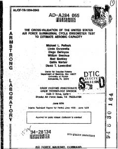
A symbolic listing of the nonzero positions of the Jacobian matrix for this example is given in Fig. 6.2.
The only significance to be
attached to the digits and letters is that there is a nonzero entry in each of the noted positions.
All other entries are zeros, so only 9.5%
of the matrix elements are nonzero and are accounted for by sparse matrix methods.
Formulation of the Optimal Design Problem:
By virtue of its move-
ment, a radial slider-crank mechanism exerts a force on ground through the crank bearing and the wrist-pin guide. "shaking forces" within bounds.
It is desirable to keep these
It is also desired that an upper bound
be placed on the angular velocity of the crank at the final instant the time-interval [0,T] under consideration.
T
of
The cost function is chosen
28 to be twice the maximum energy that is stored in the spring during the interval of motion.
The design parameters shown in Fig. 6.1, are as
follows: bI = spring constant k
of the spring
b2
-
height of the points of attachment of the spring
b3
-
half of the length of the coupler
With the notation of Sections 2 and 4, the optimal design problem is stated as follows:
0
Minimize
10)
=max b1 (.1 -
( (6.1)
O1-4
_%ALA
49
1 t
I
'
45 C~E a C .r DFPR
e F
9 C
-
0 A D E (3 ,
.Z
K L
N 0
S..0
3U 7
P
TV 8 ...
.
--
*
'C Y 56 78
S
CPQ
X..Y2 ZI
Figure 6.2
0 CE
AL 08MN -
*
.
90 AB .TJ
GHI j
UV
8
.9 K
A 3 S21Z W T R
K
L
N. w x YZ
1 2 34 COE F RST 3 45
U vw .660. 79 A
Symbolic Listing of the Nonzero Entries in the Jacobian Matrix for the Example Slider-Crank Mechanism
DISTRIBUTION LIST
Please notify USATACOM, DRSTA-ZSA, Warren, Michigan and/or changes in address.
(25) Commander US Army Tk-Autmv Command R&D Center 48090 Warren, MI (02) Superintendent US Military Academy ATTN: Dept of Engineering Course Director for Automotive Engineering (01) Commander US Army Logistic Center 23801 Fort Lee, VA US Army Research Office (02) P.O. Box 12211 ATTN: Dr. F. Schmiedeshoff Dr. R. Singleton Research Triangle Park, NC 27709 (01) HQ, DA ATTN: DAMA-AR Dr. Herschner 20310 Washington, D.C. (01) HQ, DA Office of Dep Chief of Staff for Rsch, Dev G Acquisition ATTN: DAMA-AR Dr. Charles Church 20310 Washington, D.C. HQ, DARCOM 5001 Eisenhower Ave. ATTN: DRCDE Dr. R.L. Haley 22333 Alexandria, VA
48090, of corrections
(01) Director Defense Advanced Research Projects Agency 1400 Wilson Boulevard 22209 Arlington, VA (01) Commander US Army Combined Arms Combat Developments Activity ATTN: ATCA-CCC-S 66027 Fort Leavenworth, KA (01) Commander US Army Mobility Equipment Research and Development Command ATTN: DRDME-RT 22060 Fort Belvoir, VA (02) Director US Army Corps of Engineers Waterways Experiment Station P.O. Box 631 39180 Vicksburg, MS (01) Commander US Army Materials and Mechanics Research Center ATTN: Mr. Adachi Watertown, MA 02172 (03) Director US Army Corps of Engineers Waterways Experiment Station P.O. Box 631 ATTN: Mr. Nuttall 39180 Vicksburg, MS (04) Director US Army Cold Regions Research & Engineering Lab P.O. Box 282 ATTN: Dr. Freitag, Dr. W. Harrison Dr. Liston, Library Hanover, NH 03755
(02) President Army Armor and Engineer Board 40121 Fort Knox, KY (01) Commander US Army Arctic Test Center APO 409 98733 Seattle, WA (02) Commander US Army Test & Evaluation Command ATTN: AMSTE-BB and AMSTE-TA Aberdeen Proving Ground, MD 21005 Commander (01) US Army Armament Research and Development Command ATTN: Mr. Rubin Dover, NJ 07801 (01) Commander US Army Yuma Proving Ground ATTU: STEYP-RPT 85364 Yuma, AZ Commander (01) US Army Natic Laboratories ATTN: Technical Library Natick, MA 01760 Director (01) US Army Human Engineering Lab ATTN: Mr. Eckels Aberdeen Proving Ground, MD 21005 (02) Director US Army Ballistic Research Lab Aberdeen Proving Ground, MD 21005 Director (02) US Army Materiel Systems Analysis Agency ATTN: AMXSY-CM Aberdeen Proving Ground, MD 21005
t4
Director (02) Defense Documentation Center Cameron Station 22314 Alexandria, VA (01) US Marine Corps Mobility & Logistics Division Development and Ed Command ATTN: Mr. Hickson 22134 Quantico, VA Keweenaw Field Station (01) Keweenaw Research Center Rural Route 1 P.O. Box 94-D ATTN: Dr. Sung M. Lee Calumet, MI 49913 Naval Ship Research & (02) Dev Center Aviation & Surface Effects Dept Code 161 20034 Washington, D.C. Director (01) National Tillage Machinery Lab Box 792 Auburn, AL 36830 (02) Director USDA Forest Service Equipment Development Center 444 East Bonita Avenue 91773 San Dimes, CA Engineering Societies Library 345 East 47th Street 10017 New York, NY
(01)
(01) Dr. I.R. Erlich Dean for Research Stevens Institute of Technology Castle Point Station Hoboken, NJ 07030
Grumman Aerospace Corp
(02)
South Oyster Bay Road ATTN: Dr. L. Karafiath Mr. F. Markow M/S A08/35 11714 Bethpage, NY
Mr. H.C. Hodges (01) Nevada Automotive Test Center Box 234 Carson City, NV 89701 (01)
Oregon State University (01) Library Corvallis, OR 97331 Southwest Research Inst (01) 8500 Culebra Road San Antonia, TX 78228 FMC Corporation Technical Library P.O. Box L201 San Jose, CA 95108
(01)
Box 235 Library 4455 Benesse Street Buffalo, NY 14221
Dr. Bruce Liljedahl (01) Agricultural Engineering Dept Purdue University Lafayette, IN 46207
Mr. R.S. Wismer Deere & Company Engineering Research 3300 River Drive Moline, IL 61265
CALSPAN Corporation
(01)
Mr. J. Appelblatt (01) Director of Engineering Cadillac Gauge Company P.O. Box 1027 Warren, MI 48090 Chrysler Corporation (02) Mobility Research Laboratory, Defense Engineering Department 6100 P.O. Box 751 Detroit, MI 48231
(01) SEM, Forsvaretsforskningsanstalt Avd 2 Stockholm 80, Sweden Mr. Hedwig RU 111/6 Ministry of Defense 5300 Bonn, Germany
(02)
Foreign Science & Tech (01) Center 220 7th Street North East ATTN: AMXST-GEI Mr. Tim Nix Charlottesville, VA 22901 General Research Corp (01) 7655 Old Springhouse Road Westgate Research Park ATTN: Mr. A. Viilu McLean, VA 22101 Commander (01) US Army Developmant and Readiness Command 5001 Eisenhower Avenue ATTN: Dr. R.S. Wiseman Alexandria, VA 22333