background knowledge enriched data mining

Annotation Concept Synthesis and Enrichment Analysis: a Logic-Based Approach to the Interpretation of High-Throughput Biological Experiments

Mikhail Jiline Supervisors: Stan Matwin, Marcel Turcotte

Thesis submitted to the Faculty of Graduate and Postdoctoral Studies In partial fulfillment of the requirements For the Ph.D. degree in Computer Science

School of Information Technology and Engineering Faculty of Engineering University of Ottawa

© Mikhail Jiline, Ottawa, Canada, 2011

Abstract In recent years, the amounts of information generated by biological experiments have been quickly growing. High-throughput techniques have been developed and now are extensively used to screen biological systems at a genome-wide scale. Biological studies now focus not on individual genes but on sets of genes. Extracting structured and compact knowledge from massive amounts of experimental data is a major challenge for bioinformatics. A number of algorithms and tools have been developed to process experimental data from high-throughput experiments. It seems more and more evident that no single algorithm or method can take the raw data of an experiment and convert it to a form convenient for further inspection by human experts. Instead a sequence of processing stages, complex by themselves, needs to be performed. Current approaches to the processing of high-throughput experiment data consist of two stages: primary and secondary. The primary processing stage involves normalization, conversion and filtering of raw experimental data. The secondary stage is set to structure and condense the results of large-scale experiments making them assessable by a human expert. In this thesis we concentrate on the Annotation Enrichment Analysis (AEA) approach used at the secondary stage of data processing. Annotation Enrichment Analysis is a widely used analytical methodology to process data generated by high-throughput genomic and proteomic experiments such as gene expression microarrays. The analysis uncovers and summarizes discriminating background information for sets of genes identified at the primary processing stage (e.g., a set of differentially expressed genes, a cluster). Enrichment analysis algorithms attach annotations to the genes and then discover statistical fluctuations of individual annotation terms in a given gene subset. The annotation terms represent different aspects of biological knowledge and come from databases such as GO, BIND, KEGG. Typical statistical models used to detect enrichments or depletions of annotation terms are hypergeometric, binomial and 2. At the end, the discovered information is utilized by human experts to find biological interpretations of the experiments. The main drawback of AEA is that it isolates and tests for overrepresentation of isolated individual annotation terms or groups of similar terms. As a result, AEA is limited in its ability to uncover complex phenomena involving relationships between multiple annotation terms from various knowledge bases. Also, AEA assumes that annotations describe the whole object of interest, which makes it difficult to apply it to sets of compound objects (e.g., sets of protein-protein interactions) and to sets of objects having an internal structure (e.g., protein complexes). To overcome this shortcoming, we propose a novel logic-based Annotation Concept Synthesis and Enrichment Analysis (ACSEA) approach. In this approach, the source annotation information, experimental data and uncovered enriched annotations are represented as First-Order Logic (FOL) statements. ACSEA uses the fusion of inductive logic reasoning with statistical inference to uncover more complex phenomena captured by the experiments. The proposed paradigm allows a synthesis of enriched annotation concepts that better describe the observed biological processes. ii

The methodological advantage of Annotation Concept Synthesis and Enrichment Analysis is sixfold. Firstly, it is easier to represent complex, structural annotation information. Information already captured and formalized in OWL and RDF knowledge bases can be directly utilized. Secondly, it is possible to synthesize and analyze complex annotation concepts. Thirdly, it is possible to perform the enrichment analysis for sets of aggregate objects (such as sets of genetic interactions, physical protein-protein interactions or sets of protein complexes). Fourthly, annotation concepts are straightforward to interpret by a human expert. Fifthly, the logic data model and logic induction are a common platform that can integrate specialized analytical tools (e.g. tools for numerical, structural and sequential analysis). Sixthly, used statistical inference methods are robust on noisy and incomplete data, scalable and trusted by human experts in the field. In this thesis we developed and implemented the ACSEA approach. We evaluate it on largescale datasets from several microarray experiments and on a clustered genome-wide genetic interaction network using different biological knowledge bases. Also, we define a statistical model of experimental and annotation data and evaluate ACSEA on synthetic datasets. The discovered interpretations are more enriched in terms of P- and Q-values than the interpretations found by AEA, are highly integrative in nature, and include analysis of quantitative and structured information present in the knowledge bases. The results suggest that ACSEA can significantly boost the effectiveness of the processing of high-throughput experiment data.

iii

Acknowledgments First and foremost I wish to express my sincere gratitude to my supervisors, Pr. Stan Matwin and Pr. Marcel Turcotte. I am indebted to Stan, whose knowledge, guidance, encouragement and positive attitude helped me through all these years. I am also grateful for an exceptional example he provided as a successful researcher, professor, organizer and leader. I owe my deepest gratitude to Marcel who introduced me to a wonderful world of bioinformatics and computational biology. A small directed study project completed under his supervision was the seed for the ideas that eventually, after few years, became the foundation of this thesis. I would like to thank the members of my committee, Pr. Gary Bader, Pr. Michel Dumontier, Pr. Thomas Tran, and Pr. Fazel Famili for their time, thoughtful comments and insightful and entertaining discussion. Their ideas and feedback not only helped me to improve the thesis but provided inspiration for further research. This thesis would have remained a dream had it not been for my business partner Mike Sandler and many of my colleagues at Epiphan Systems Inc., who were exceptionally accommodating and caring for my undertaking. They provided me with the resources required for this work. Their spirit and confidence fueled me during all these years. Thanks are also due to the researchers and software engineers whose datasets and software made this work feasible: Ashwin Srinivasan (Aleph), researchers at the University of Porto (YAP), Robert C. Gentleman and colleagues (R and Bioconductor), Kasper Daniel Hansen (ALL dataset), the GSEA Team at the Broad Institute (GSEA datasets), Michael Costanzo and colleagues (DRYGIN dataset). Also, I would like to mention my friend, Egor Anoshkin, whose promise to deliver a case of Champagne the moment I get my Ph.D. degree was a major motivating factor. Unfortunately, the case has not been yet delivered as of the moment of this writing. Last, but not least, I am very grateful to my family: my parents and my brother who always believed in me and encouraged through all the way; my wife, Dr. Svetlana Kiritchenko, who was the very first person I was bringing my ideas to and who made everything possible to help me make it this far, and to my daughter Anastasia, who is no doubt the most patient and understanding person in the whole world.

iv

Table of Contents ABSTRACT ............................................................................................................................................... II ACKNOWLEDGMENTS ............................................................................................................................ IV TABLE OF CONTENTS ............................................................................................................................... V LIST OF FIGURES ...................................................................................................................................VIII 1

INTRODUCTION ............................................................................................................................. 1 1.1 MOTIVATION .......................................................................................................................................1 1.1.1 High-throughput Experiments .................................................................................................2 1.1.1.1 1.1.1.2

1.1.2 1.1.2.1 1.1.2.2 1.1.2.3

1.2 1.3 2

Gene Expression Profiling .................................................................................................................. 2 Synthetic Genetic Arrays ................................................................................................................... 3

Data Mining and Knowledge Extraction for High-throughput Experiment Data ....................3 Primary Processing Stage .................................................................................................................. 4 Secondary Processing Stage .............................................................................................................. 4 Annotation Enrichment Analysis ....................................................................................................... 5

CONTRIBUTION.....................................................................................................................................5 THESIS ORGANIZATION ..........................................................................................................................7 BACKGROUND INFORMATION....................................................................................................... 8

2.1 STATISTICAL ENRICHMENT TESTS .............................................................................................................8 2.1.1 Statistical Hypothesis Testing..................................................................................................8 2.1.1.1 2.1.1.2 2.1.1.3 2.1.1.4 2.1.1.5

2.1.2 2.1.2.1

Notation ............................................................................................................................................ 9 Hypergeometric Test ......................................................................................................................... 9 Binomial Test ................................................................................................................................... 10 Fisher Exact Test .............................................................................................................................. 10 2 x Test .............................................................................................................................................. 11

Multiple Comparisons Problem .............................................................................................11 False Discovery Rate ........................................................................................................................ 12

2.2 INDUCTIVE LOGIC PROGRAMMING .........................................................................................................12 2.2.1 First Order Logic ....................................................................................................................13 2.2.1.1 2.2.1.2 2.2.1.3 2.2.1.4 2.2.1.5

2.2.2 2.2.3 2.2.4 2.2.4.1 2.2.4.2 2.2.4.3 2.2.4.4 2.2.4.5

2.2.5 2.2.5.1 2.2.5.2

2.2.6 2.2.6.1 2.2.6.2 2.2.6.3 2.2.6.4 2.2.6.5 2.2.6.6

Syntax .............................................................................................................................................. 13 Semantics ........................................................................................................................................ 14 Clausal Logic .................................................................................................................................... 14 -subsumption ................................................................................................................................ 15 Description Logics............................................................................................................................ 15

Formal Framework of ILP ......................................................................................................15 ILP Hypothesis Search ...........................................................................................................16 ILP Algorithms .......................................................................................................................17 Representation of Background Knowledge, Examples and Hypothesis .......................................... 17 Generalization/Specialization Relation and Operator ..................................................................... 17 Hypothesis Goodness Measures ..................................................................................................... 17 Search Strategy................................................................................................................................ 18 Other Variations .............................................................................................................................. 19

Combined ILP Approaches .....................................................................................................19 Support Vector Inductive Logic Programming ................................................................................. 20 Probabilistic Inductive Logic Programming ..................................................................................... 20

ILP Advantages and Disadvantages ......................................................................................21 Flexibility of the Representation ..................................................................................................... 21 Homogeneity of the Representation ............................................................................................... 22 Human Interpretability .................................................................................................................... 22 Computational Complexity .............................................................................................................. 22 Intolerance to Noise ........................................................................................................................ 23 Handling of Numerical Data ............................................................................................................ 23

v

2.2.7 2.2.7.1 2.2.7.2 2.2.7.3 2.2.7.4 2.2.7.5

3

Applications of ILP .................................................................................................................24 NLP and Text Mining ....................................................................................................................... 24 Social Network Mining .................................................................................................................... 24 Chemistry ........................................................................................................................................ 24 Molecular Biology ........................................................................................................................... 25 Genome Wide Protein Function Prediction .................................................................................... 26

ANNOTATION ENRICHMENT ANALYSIS ....................................................................................... 27 3.1 PRINCIPAL APPROACH..........................................................................................................................27 3.2 ALGORITHM VARIATIONS......................................................................................................................28 3.2.1 Databases .............................................................................................................................28 3.2.2 Data Representation Models ................................................................................................29 3.2.3 Statistical Models ..................................................................................................................30 3.2.4 Universe Set...........................................................................................................................30 3.3 DISCUSSION .......................................................................................................................................31

4

ANNOTATION CONCEPT SYNTHESIS AND ENRICHMENT ANALYSIS (ACSEA) ................................ 32 4.1 LOGIC-BASED KNOWLEDGE REPRESENTATION ..........................................................................................32 4.2 ANNOTATION CONCEPT SYNTHESIS AND ENRICHMENT ANALYSIS ALGORITHM ................................................35 4.2.1 Enrichment Analysis as a Logical-Statistical Inference Problem ...........................................35 4.2.2 Inductive Logic Programming ...............................................................................................37 4.2.3 Statistical Inference ...............................................................................................................37 4.2.4 Details of the Annotation Concept Synthesis and Enrichment Analysis Algorithm ...............38 4.2.4.1 4.2.4.2 4.2.4.3 4.2.4.4 4.2.4.5 4.2.4.6 4.2.4.7

4.3 4.4 5

Annotation Concept Synthesis ........................................................................................................ 38 Hypothesis Fitness Measure ........................................................................................................... 39 Hypothesis Lattice Properties ......................................................................................................... 39 Theory Building Strategy ................................................................................................................. 45 Integration of Specialized Algorithms ............................................................................................. 45 Controlling the Quality of the Theory ............................................................................................. 46 Search Space Tractability ................................................................................................................ 46

ANNOTATION CONCEPT SYNTHESIS AND ENRICHMENT ANALYSIS SYSTEM ......................................................47 CONCLUSION .....................................................................................................................................50 ACSEA FOR MICROARRAY ANALYSIS ........................................................................................... 51

5.1 METHODS .........................................................................................................................................51 5.1.1 Datasets and Annotation Sources .........................................................................................51 5.1.2 Evaluation Measures .............................................................................................................52 5.1.2.1 5.1.2.2

5.2 5.3 6

RESULTS............................................................................................................................................55 CONCLUSION .....................................................................................................................................57 ACSEA FOR INTERACTOME .......................................................................................................... 59

6.1 6.2 6.3 6.4 6.5 7

Review of the Evaluation Techniques Used in the Field .................................................................. 52 ACSEA Evaluation Measures for Real-World Datasets .................................................................... 54

MOTIVATION .....................................................................................................................................59 METHODS .........................................................................................................................................60 RESULTS............................................................................................................................................61 EVALUATION OF SLIDING WINDOW THEORY CONSTRUCTION.......................................................................62 CONCLUSION .....................................................................................................................................62 EVALUATION OF ENRICHMENT ANALYSIS TECHNIQUES ON SYNTHETIC DATA ............................ 64

7.1 MOTIVATION .....................................................................................................................................64 7.1.1 Indirect Evaluation of Results ................................................................................................64 7.1.2 Performance Profile of an Algorithm ....................................................................................65 7.1.3 Discoverability of the Phenomena Captured by Experimental Data. ....................................65

vi

7.2 METHODS .........................................................................................................................................66 7.2.1 Synthetic Data .......................................................................................................................67 7.2.1.1 7.2.1.2 7.2.1.3 7.2.1.4

Model of Annotational Information ................................................................................................ 68 Model of the Universe Set and Annotation Associations ................................................................ 69 Model of Biological Phenomena ..................................................................................................... 70 Model of Experimental Data ........................................................................................................... 71

7.2.2 Evaluation Measures .............................................................................................................71 7.3 RESULTS............................................................................................................................................73 7.3.1 Comparison of AEA and ACSEA on Synthetic Data ................................................................74 7.3.2 Effects of the Parameters of the Experiment ........................................................................75 7.3.2.1 7.3.2.2 7.3.2.3

Level of Experimental Noise ............................................................................................................ 76 Size of Annotational Information .................................................................................................... 78 Complexity of the Biological Phenomena ........................................................................................ 79

7.3.3 Evaluation of Pruning Effectiveness ......................................................................................81 7.4 CONCLUSION .....................................................................................................................................82 8

THEORY CONSTRUCTION FOR ACSEA ........................................................................................... 84 8.1 MOTIVATION .....................................................................................................................................84 8.2 METHODS .........................................................................................................................................84 8.2.1 Enrichment Theory Construction by Annotation Clustering ..................................................85 8.2.2 Clustering Algorithm .............................................................................................................85 8.2.2.1 8.2.2.2

8.2.3

Partitioning Around Medoids .......................................................................................................... 86 K-means Clustering .......................................................................................................................... 87

Annotation Distance Measure ..............................................................................................87

8.2.3.1 8.2.3.2

Semantic Overlap Distance.............................................................................................................. 88 Semantic-Euclidean Distance and Space ......................................................................................... 91

8.2.4 Selection of Representative Annotations ..............................................................................91 8.3 RESULTS............................................................................................................................................92 8.3.1 Comparison of Clustering-Based Theory Construction Algorithms .......................................93 8.3.2 Comparison of ACSEA-PP, ACSEA and AEA ............................................................................95 8.4 CONCLUSION .....................................................................................................................................97 9

CONCLUSION ............................................................................................................................... 98

10

APPENDIX .................................................................................................................................. 102 10.1 10.2 10.3

GSEA P53 DATASET ANALYSIS USING GO+CHR KNOWLEDGE BASES. ...................................................104 GSEA LUNG CANCER DATASET ANALYSIS USING GO+CHR KNOWLEDGE BASES ......................................113 INTERACTOME ANALYSIS USING GO+CHR KNOWLEDGE BASE ..............................................................123

BIBLIOGRAPHY .................................................................................................................................... 136

vii

List of Figures FIGURE 1-1 DATA MINING FOR HIGH-THROUGHPUT EXPERIMENT DATA. ..............................................................................4 FIGURE 2-1. MOLECULES OF (A) WATER, (B) BENZENE AND (C) TRYPTOPHAN AMINO ACID ......................................................22 FIGURE 3-1. ANNOTATION ENRICHMENT ANALYSIS APPROACH. ........................................................................................27 FIGURE 3-2. BAG-OF-ANNOTATION-TERMS DATA MODEL .................................................................................................29 FIGURE 4-1. LOGIC-BASED REPRESENTATION OF STRUCTURAL INFORMATION........................................................................35 FIGURE 4-2. ANNOTATION CONCEPT INFERENCE. ...........................................................................................................36 FIGURE 4-3. THE MAPPING BETWEEN THE LATTICE AND . .......................................................................................43 FIGURE 4-4. MONOTONICALLY NON-INCREASING PATHS IN AND SUBSPACES. .................................................... 44 FIGURE 4-5. ACSEA SYSTEM DIAGRAM .......................................................................................................................49 FIGURE 5-1. AN EXAMPLE OF A SYNTHESIZED ANNOTATION CONCEPT FOR A MICROARRAY EXPERIMENT .....................................55 FIGURE 5-2. PVAVRN MEASURES FOR MICROARRAY EXPERIMENTS. .....................................................................................56 FIGURE 5-3. QVAVRN MEASURES FOR MICROARRAY EXPERIMENTS. ....................................................................................56 FIGURE 5-4. PVAVRN MEASURES FOR MICROARRAY EXPERIMENTS ON A LOGARITHMIC SCALE...................................................56 FIGURE 5-5. QVAVRN MEASURES FOR MICROARRAY EXPERIMENTS ON A LOGARITHMIC SCALE. .................................................57 FIGURE 6-1. AN EXAMPLE OF A SYNTHESIZED ANNOTATION CONCEPT FOR A GENE INTERACTION EXPERIMENT. ............................61 FIGURE 7-1. DIRECT (A) AND INDIRECT (B) ALGORITHM EVALUATION. ...............................................................................65 FIGURE 7-2. EVALUATION OF ENRICHMENT ANALYSIS TECHNIQUES ON SYNTHETIC DATA .......................................................67 FIGURE 7-3 SMALL SCALE EXAMPLES OF SYNTHESIZED GRAPHS...........................................................................................69 FIGURE 7-4 ANNOTATION ASSOCIATIONS BETWEEN OBJECTS OF UNIVERSE SET AND ANNOTATIONAL INFORMATION. ....................70 FIGURE 7-5 DIRECT EVALUATION OF ENRICHMENT ANALYSIS TECHNIQUES ON SYNTHETIC DATA..............................................73 FIGURE 7-6. LPVAVRN MEASURES FOR ALL SYNTHETIC EXPERIMENTS...................................................................................74 FIGURE 7-7. LQPVAVRN MEASURES FOR ALL SYNTHETIC EXPERIMENTS. ...............................................................................74 FIGURE 7-8. PAMCN MEASURES FOR ALL SYNTHETIC EXPERIMENTS. ...................................................................................75 FIGURE 7-9. APDR90%,N FOR ALL SYNTHETIC EXPERIMENTS. ..............................................................................................75 FIGURE 7-10. DEPENDENCY OF LPVAVRN ON THE LEVEL OF NOISE FOR AEA AND ACSEA. ......................................................76 FIGURE 7-11. DEPENDENCY OF LQVAVRN ON THE LEVEL OF NOISE FOR AEA AND ACSEA. .....................................................76 FIGURE 7-12. DEPENDENCY OF PAMCN ON THE LEVEL OF NOISE FOR AEA AND ACSEA. .......................................................76 FIGURE 7-13. DEPENDENCY OF APDR90%,N ON THE LEVEL OF NOISE FOR AEA AND ACSEA. ...................................................77 FIGURE 7-14. PAMCN MEASURED ON ALL DATA VERSUS LOW AND MODERATE NOISE DATA. ...................................................77 FIGURE 7-15. APDR90%, MEASURED ON ALL DATA VERSUS LOW AND MODERATE NOISE DATA. ................................................78 FIGURE 7-16. DEPENDENCY OF LPVAVRN ON THE SIZE OF ANNOTATIONAL INFORMATION. ......................................................78 FIGURE 7-17. DEPENDENCY OF LQVAVRN ON THE SIZE OF ANNOTATIONAL INFORMATION. .....................................................78 FIGURE 7-18. DEPENDENCY OF PAMCN ON THE SIZE OF ANNOTATIONAL INFORMATION. .......................................................79 FIGURE 7-19. DEPENDENCY OF APDR90%,N ON THE SIZE OF ANNOTATIONAL INFORMATION. ...................................................79 FIGURE 7-20. DEPENDENCY OF LPVAVRN ON THE COMPLEXITY OF BIOLOGICAL PHENOMENA. ..................................................80 FIGURE 7-21. DEPENDENCY OF LQVAVRN ON THE COMPLEXITY OF BIOLOGICAL PHENOMENA. .................................................80 FIGURE 7-22. DEPENDENCY OF PAMCN ON THE COMPLEXITY OF THE BIOLOGICAL PHENOMENA...............................................80 FIGURE 7-23. DEPENDENCY OF APDR90%,N ON THE COMPLEXITY OF THE BIOLOGICAL PHENOMENA. .........................................81 FIGURE 7-24. NUMBER OF HYPOTHESES EXPLORED BY THE ACSEA ALGORITHM. ..................................................................82 FIGURE 8-1. COVERAGE SET COMPOSITION....................................................................................................................89 FIGURE 8-2. LPVAVRN MEASURES FOR ENRICHMENT THEORY CONSTRUCTION ALGORITHMS. ..................................................93 FIGURE 8-3. LQVAVRN MEASURES FOR ENRICHMENT THEORY CONSTRUCTION ALGORITHMS. .................................................94 FIGURE 8-4. PAMCN MEASURES FOR ENRICHMENT THEORY CONSTRUCTION ALGORITHMS. ...................................................94 FIGURE 8-5. APDR90%,N MEASURES FOR ENRICHMENT THEORY CONSTRUCTION ALGORITHMS. ...............................................94 FIGURE 8-6. LPVAVR,N MEASURES FOR AEA, ACSEA, ACSEA-PP. ...................................................................................95 FIGURE 8-7. LQVAVRN MEASURES FOR AEA, ACSEA, ACSEA-PP. ...................................................................................96 FIGURE 8-8. PAMCN MEASURES FOR AEA, ACSEA, ACSEA-PP. .....................................................................................96 FIGURE 8-9. APDR90%,N MEASURES FOR AEA, ACSEA, ACSEA-PP. .................................................................................96 FIGURE 8-10. APDR90%,N MEASURES FOR AEA, ACSEA, ACSEA-PP DEPENDING ON PHENOMENA COUNT...............................97

viii

List of Tables TABLE 2-1. CONTINGENCY TABLE ................................................................................................................................10 TABLE 2-2 ILP GENERALIZATION MEASURES..................................................................................................................18 TABLE 2-3 ILP SEARCH SPACE ENUMERATION ALGORITHMS .............................................................................................19 TABLE 4-1. TYPICAL TYPES OF BACKGROUND KNOWLEDGE. ...............................................................................................34 TABLE 4-2. LOGIC-BASED REPRESENTATION OF GENE ONTOLOGY ......................................................................................34 TABLE 5-1. MICROARRAY DATASETS ............................................................................................................................51 TABLE 5-2. SOURCES OF ANNOTATIONS ........................................................................................................................52 TABLE 5-3. QUANTITATIVE PERFORMANCE EVALUATION OF AEA AND ACSEA ON GENE EXPRESSION MICROARRAY DATASETS. SMALLER IS BETTER...........................................................................................................................................58 TABLE 6-1. ANNOTATION DATABASES FOR GENETIC INTERACTION SCREENS.........................................................................60 TABLE 6-2. QUANTITATIVE PERFORMANCE EVALUATION OF AEA AND ACSEA ON GENETIC INTERACTION SCREENS ....................61 TABLE 8-1. CLUSTERING-BASED THEORY CONSTRUCTION ALGORITHMS ..............................................................................93 TABLE 8-2. PAIRED T-TEST BETWEEN ACSEA-KP AND ACSEA-PP ....................................................................................95

ix

1 Introduction In this chapter we provide: 



A motivation for the thesis mainly stemming from information processing challenges faced by molecular biology. We include a brief description of typical experiments and datasets used in the field. We discuss conventional bioinformatics approaches, including a short overview of Annotation Enrichment Analysis. We conclude the motivation section by identifying some limitations in the existing approaches. A list of contributions of the thesis.

1.1 Motivation In recent years, the amounts of available information in biological datasets have been quickly growing. The datasets containing genome sequences, protein sequences, protein secondary and three-dimensional structures, protein motifs, metabolic pathways, interaction networks, and curated literature are updated and extended on a daily basis. At the same time, it is increasingly clear that no significant biological function can be attributed to one molecule. Each function is the result of complex interactions between all types of biological molecules, such as DNA, RNA, proteins, lipids and carbohydrates. Biological functions have to be studied taking into consideration the cell as a whole, including its static composition and, even more importantly, dynamic behavior. New large-scale experimental techniques have been developed and now are widely accepted and used. High-throughput methods, such as expression microarrays, promoter microarrays, genome-wide physical and genomic interaction screens, while allowing to monitor the behavior of the cell as a whole, are generating wealth of information that needs to be studied and interpreted. Given all these circumstances, it is evident that a reductionist approach (also known as divideand-conquer approach), which served very well the scientific community for ages, may not be used so productively in modern molecular biology. While it has been used successfully to identify and describe parts of the molecular machinery, there is simply no way reductionism can help us understand how the system properties emerge from interactions of myriad of relatively basic elements. The modern molecular biology approach is quite the opposite to reductionism. Instead of moving from complex behavior/system to simpler ones, modern genomics and proteomics try to reconstruct and understand complex behavior by observing how elementary pieces of the system operate and interact with each other. Speaking in terms of molecular biology, entire systems of genes, proteins, enzymes and metabolites are observed to infer metabolic pathways, and then in turn more complex interactions are found between pathways, regulatory mechanisms, and mechanisms of cell specialization and interaction. Therefore, one of the main challenges of

1

bioinformatics is to develop methods and techniques that can help to infer knowledge from accumulated datasets and large-scale experimental data. In this thesis we will concentrate on bioinformatics enrichment algorithms that help biologists analyze the results of experiments by discovering patterns of already known information in newly obtained data sets.

1.1.1 High-throughput Experiments In this section we briefly describe several modern high-throughput experimental techniques. We concentrate on characteristics of the data generated by the experiments and on data processing challenges, while trying to avoid peripheral (with respect to this thesis) technological, biological and chemical details of the techniques. More information can be found in the referenced papers. Modern molecular biology high-throughput screening techniques include gene expression microarrays (Schena, 1996), RNA-Seq (Wang, Gerstein, & Snyder, 2009), promoter microarrays, ChIP-on-chip (Buck & Lieb, 2004), RIP-Chip, synthetic genetic arrays (Tong & al., 2004), syntheticlethality analysis by microarray (Ooi, Shoemaker, & Boeke, 2003), two-hybrid screening (Young, 1998), (Joung, Ramm, & Pabo, 2000). While there are many high-throughput screening technologies we choose only two of them for further discussion, as these two are popular and representative (from the data analysis point of view) of the two major classes of the experiments.

1.1.1.1 Gene Expression Profiling In molecular biology, one of the applications of DNA microarrays is gene expression profiling. DNA microarrays allow to simultaneously monitor the level of expression for thousands of genes. Typical experiments monitor gene expression profiles of the similar cells in several distinct conditions (for example, in presence and absence of a drug or at different temperatures). Monitoring of gene expression profiles of distinct cells (for example, cells of different tissues or diseased and healthy cells of the same tissue) is also a widely applied protocol. A data analysis phase consists of studying and comparing the captured expression profiles. The profiles allow to observe how the condition affects gene expression levels of the whole cell at once, and consequently infer genomics and proteomics knowledge such as insights into the functioning of genes, proteins, topology of metabolic networks, etc. (Schena, 1996). From a bioinformatics point of view, the output of a DNA microarray experiment is represented by a numeric table. In this table, thousands of genes are represented by rows. Different time points or conditions are represented by columns (typically, there are just a few of them comparing to the number of genes). Cells of the table contain detected gene expression levels. Due to the significant disproportion between the dimensions, such tables are often called “fat tables”. Typically, the knowledge extraction from such tables starts from the noise filtration and level normalization (Quackenbush, 2002), followed by the outlier type analysis (selecting a differentially expressed subset of genes) or the clustering/partitioning analysis (detecting subsets of genes displaying somehow similar behavior).

2

1.1.1.2 Synthetic Genetic Arrays Synthetic Genetic Arrays is a high-throughput in-vivo technique for detecting genetic interactions between pairs of genes (Tong & al., 2004). Generally, the experiments consist of modifying a cell’s genotype and observing changes in the cell’s phenotype. Typical examples of genetic interactions are synthetic lethality and synthetic dosage lethality screens. Both screens detect genes that cause lethality (or some sort of sickness for dosage lethality screens) of the cell when simultaneously mutated (knocked off), but do not cause lethality when only one of the mutations is present. Such relation between genes may indicate some sort of interoperation between genes in a metabolic pathway. For example, synthetic lethal interactions may be considered as evidence supporting two hypotheses (Tucker & Fields, 2003), (Ye, Peyser, Pan, Boeke, Spencer, & Bader, 2005):  

two genes in a single linear pathway can show synthetic lethality; synthetic lethal genes act in parallel or compensating pathways.

The output of a Synthetic Genetic Array experiment is a table where one set of genes is represented by rows, another set of genes is represented by columns. Cells of the table contain an indication of the detected interaction between tested genes. Similar data are produced by physical interaction screening techniques (e.g. two-hybrid screening). Typically, the knowledge extraction from such tables includes the noise filtration, data normalization(Quackenbush, 2002), and the significance analysis of the evidences of detected interactions(Kooperberg & Sipione, 2002). It results in a simplified Boolean table reflecting detected interactions. Consequently, the clustering/partitioning analysis is applied to detect genes with similar interaction patterns.

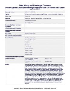
1.1.2 Data Mining and Knowledge Extraction for Highthroughput Experiment Data Due to sheer volume of data generated by high-throughput experiments (dozens of thousands of genes, hundreds of thousands of interactions), it is virtually impossible for a human expert to directly analyze the data. Due to the very same volume of data, as well as large amount of noise and a wide semantic gap between raw data and useful knowledge that needs to be extracted, the automatic processing of biological datasets is not an easy task. It seems more and more evident that no single algorithm can take raw experimental data and convert them to a form suitable for further inspection by human experts. Instead, a sequence of processing stages, complex by themselves, needs to be performed (Khatri & Draghici, 2005). Thus, modern approaches to the processing of data obtained from high-throughput experiments may be viewed as a two-stage analysis. We name the stages primary and secondary. The following sections as well as Figure 1-1 explain the goals of each stage.

3

Conclusion: Primary Processing Stage

Secondary Processing Stage

genes in cluster A are involved in “membrane biogenesis process”

Raw data Clustered genes or sets of differentially expressed genes

Annotation Databases GO, KEGG, BIND

Figure 1-1 Data Mining for High-throughput Experiment Data.

1.1.2.1 Primary Processing Stage The main goal of the primary processing stage is to digitize, normalize and filter raw experimental data. The stage consists of applying a series of algorithms and data transformations. Good awareness of the physical/biological/chemical properties of a high-throughput technique is a common feature of the algorithms used at the primary processing stage. For example, the primary processing for DNA microarray experiments typically involves the following steps (Hegde, et al., 2000 ): integration of spot intensities, normalization of relative intensities, clustering, and identification of differentially expressed genes. The typical results of the primary processing stage are sets of differentially expressed genes, or flat or hierarchical clusters of genes. For synthetic genetic screens and synthetic-lethality analysis by microarray the primary processing may include integration of spot intensities, normalization of intensities, 2D clustering, and the interaction map analysis (Ma, Tarone, & Li, 2008). Typically, the results of the primary processing stage are interaction maps and clusters of gene interactions.

1.1.2.2 Secondary Processing Stage While the primary processing stage rectifies the raw output of high-throughput experiments, in most cases the results of the processing are still large-scale data arrays. Gene expression clusters still contain hundreds of genes. The results of genetic interaction screens, even when clustered, contain hundreds of interactions as well. Essentially, the data obtained after the primary processing stage are just a starting point for a meaningful biological investigation. The secondary stage of processing is designed to structure and condense the results of an experiment as much as possible, effectively making the results of a large-scale experiment assessable by a human expert. A common feature of modern algorithms used at the secondary

4

processing stage is the abstraction from a particular experimental technique and the involvement of the background knowledge to the data analysis.

1.1.2.3 Annotation Enrichment Analysis One of the most popular secondary processing techniques is Annotation Enrichment Analysis (AEA) (Khatri & Draghici, 2005), (Huang, Sherman, & Lempicki, 2009). AEA uses the biological knowledge already accumulated in public databases to systematically examine large lists of genes (assembled at the primary processing stage) trying to suggest biological interpretations of the experimental data. AEA algorithms extract descriptive information (called annotations) characterizing each gene and compare the statistical distributions of gene annotations between the gene set of interest (known as study set) and the rest of the genome or the rest of the microarray (known as universe set). Detected statistical overrepresentations (or enrichments) are of immense worth to investigators trying to identify biological phenomena related to their study. The data representation model used in Annotation Enrichment Analysis is bag-of-annotations. By analogy with a bag-of-words representation used in text mining, bag-of-annotations associates a set of annotation terms with each gene. While bag-of-annotations is a very popular and efficient model allowing natural application of statistical inference methods, it has a number of disadvantages. The main weakness of the model is the limitation in the types of annotation terms and relations that may be used as well as the types and the complexity of enriched phenomena that can be discovered and described. As a result, AEA isolates and tests for overrepresentation of isolated individual annotation terms or groups of similar terms and is limited in its ability to uncover complex phenomena involving relationships between multiple annotation terms from various knowledge bases. Also, AEA assumes that annotations describe the whole object of interest, which makes it difficult to apply it to sets of compound objects (e.g. sets of protein-protein interactions) and to sets of objects having an internal structure (e.g. protein complexes). In this thesis we are aming to address these shortfalls by a fundamental change in the underlying annotation data model from bag-ofannotations to First-Order Logic and develop knowledge extraction algorithms operating on the improved data model.

1.2 Contribution This thesis makes the following six major contributions: 1. We recognize a limitation of all AEA algorithms stemming from the universally utilized data model and propose a more flexible data model based on First-Order Logic (FOL). Such fundamental change of the underlying data representation allows to significantly improve:  

Completeness and coherence of representation of accumulated knowledge (the knowledge used as a base for annotations); Specificity of annotation terms; 5



Precision of associations between annotation terms and annotated objects (or parts of thereof).

We show how well-known knowledge bases (e.g., Gene Ontology) can be represented by the means of logic and how all representation improvements specified above translate into more complete, specific and precise enriched annotations. 2. We propose a novel Annotation Concept Synthesis and Enrichment Analysis (ACSEA) paradigm. ACSEA fuses inductive logic reasoning and statistical inference. Such a combined approach allows us to take advantage of a richer, logic-based data representation model. This, in turn, translates into the ability to uncover more complex phenomena captured by the biological experiment. We evaluate our approach on large-scale datasets from several microarray experiments and on a clustered genome-wide genetic interaction network using different biological knowledge bases. We show that the discovered interpretations have lower P-values than the interpretations found by AEA, are highly integrative in nature, and include analysis of quantitative and structured information present in the knowledge bases. 3. We propose an innovative application of the ILP theory. While normally ILP techniques are used for classification tasks involving relational data, this research shows how an approach that incorporates inductive logic techniques can serve as a knowledge integration mechanism, enriching data with relational background knowledge and resulting in comprehensible interpretations of experimental data. 4. We define a statistical model to generate synthetic data simulating the results of highthroughput microarray experiments. The generated data includes background knowledge, experimental data and biological phenomena. The model is parameterized by the size of background knowledge, the size of experimental data, the amount of noise in experimental data, and the number of biological phenomena captured by the experiment. The synthetic data is essential for advanced studies of enrichment analysis techniques, as parameters of the data as well as correct enrichments are known and can be used to better evaluate the performance of the algorithms. Based on the model, we generate synthetic data and compare the performance of the AEA and ACSEA approaches. 5. We study the problem of discoverability of the phenomena captured by experimental data using the enrichment analysis approach. We define measures specifically aimed to quantitatively assess how closely the discovered enriched annotations reflect the biological phenomena captured by the experiment (biological phenomena are not directly observable by AEA and ACSEA). Using the measures we show the general effectiveness of the enrichment analysis with respect to the parameters of the model (the size of the data, noise, etc.), as well as compare AEA and ACSEA under the controlled variety of conditions. 6. We propose a distinct Enrichment Theory Construction Step to avoid over-fitting of the Enrichment Theory to one or a few of the most enriched phenomena discovered. Conventional AEA algorithms implicitly form an enrichment theory by sorting enrichments according to their P-values, consequently cutting the list at a predefined P-value threshold or at a specified a priori length. In this thesis, we develop a dedicated theory construction strategy. The proposed theory construction algorithm is based on the clustering techniques 6

and designed to detect distinct phenomena captured by the experiment and select the best enrichments representing each phenomena. We compare the quality of the enrichment theories obtained by the conventional and the proposed theory building strategies on synthetic data and show that the addition of the Enrichment Theory Construction Step results in a more diverse and more valuable enrichment theory. The main conclusion of this thesis is that the logic-based representation, inductive logic reasoning and statistical inference can be productively fused and consequently applied to the analysis of biological experiments. Such an approach boosts the effectiveness and efficiency of the processing of high-throughput experiments and opens up the doors to extending the enrichment analysis to other types of experiments (such as the analysis of interactome and protein complexes data).

1.3 Thesis Organization The remainder of the thesis is organized as follows. Chapter 2 briefly reviews the major theories, concepts and algorithms referred or relevant for the thesis. It establishes common terminology and definitions used throughout the thesis. Chapter 3 contains the overview of Annotation Enrichment Analysis algorithms as well as related previous work. Chapter 4 describes the proposed approach, Annotation Concept Synthesis and Enrichment Analysis (ACSEA). Chapter 5 presents the results of the evaluation of ACSEA on several real-world microarray datasets. Chapter 6 discusses the extension of ACSEA for the analysis of sets of aggregate objects such as interactome datasets. It also presents the evaluation of ACSEA on Data Repository of Yeast Genetic INteractions (DRYGIN) database. Chapter 7 discusses the study of the Enrichment Analysis techniques on synthetic data. Chapter 8 describes a novel approach to Enrichment Theory construction based on clustering of enriched annotation concepts. Finally, Chapter 9 summarizes the findings and contributions of this thesis.

7

2 Background Information This chapter briefly reviews the major theories, concepts and algorithms referred or relevant for the thesis. It establishes common terminology and definitions used throughout the thesis.

2.1 Statistical Enrichment Tests The goal of statistical enrichment analysis is to detect and rate significant abnormalities in the distributions of known information in the subset of interest (e.g. a set of differentially expressed genes) comparing to the same distributions in the set of all objects (e.g. all genes). We will provide details of annotation enrichment analysis in the following chapter. In this chapter we will review generic statistical methods used to detect and rate under- and overrepresentations, see (Lehmann & Romano, 2005) and (Rivals, Personnaz, Taing, & Potier, 2007) for a thorough presentation.

2.1.1 Statistical Hypothesis Testing Statistical enrichment analysis relies on statistical hypothesis testing methodologies (specifically on null-hypotheses tests) to detect a significant enrichment of annotation terms. Generally, the null-hypothesis test consists of the following steps: 1. Define a null hypothesis H0, which we will try to disprove during the test. The null hypothesis is selected to contrast the tested (alternative) hypothesis H1. For Enrichment Analysis, the null hypothesis usually states that the property of a gene to have specific annotation and its property to belong to the study set are independent. The tested hypothesis states that these properties are dependent and thus the annotation have different distributions in the study set and in universe set. 2. Select a statistic that will be used to test hypothesis. For Enrichment Analysis, it is the number of times an annotation appears in the study set. 3. Assuming that the null hypothesis is correct, compute the probability (P-value) of observing a value for the test statistic that is as extreme or more extreme as the value that was actually observed. For Enrichment Analysis, this step relies on the universe set and statistical distribution model to compute the probability. In this way, we arrive at quantitative opinion as to whether the frequency of occurrence of an annotation in the study set is significantly different from that in the universe set. Different semantics of “Extreme” (extreme on one tail or both tails of distribution) lead to one- or two-sided tests. They can be used to detect enrichments, depletions, or enrichment or depletion of the annotations.

8

A specific distribution model is required to compute a P-value. In the next few sections we will describe several frequently used distributions such as hypergeometric and binomial. 4. Based on the computed P-value, the null hypothesis can be rejected if the P-value falls below a significance threshold (critical value). Non-threshold tests can also ne used (Subramanian, et al., 2005).

2.1.1.1 Notation For the next sections we will use the following notation: Denote the control set as C, Denote the study set as S,

. .

Suppose the annotation term for which we compute the P-value is t. Let Ct be the set of genes annotated with term t. Then

.

Let St be the subset of S that includes only genes annotated with the term t, .

. Then

2.1.1.2 Hypergeometric Test The hypergeometric test assumes the hypergeometric distribution on samples to determine the probability of observing a value for the test statistic. The hypergeometric distribution is a discrete distribution that describes the number of positive draws in a sequence of draws from a finite population of positive and negative outcomes without replacement. According to the hypergeometric distribution model, the probability of observing exactly annotations can be computed as follows: (2.1) The probability of observing

or more annotations can be computed as follows:

(2.2)

is the P-value of significant enrichment of the annotation term t in the study set S, according to the one-sided hypergeometric test.

9

2.1.1.3 Binomial Test The binomial test assumes the binomial distribution on samples to determine the probability of observing a value for the test statistic. The binomial distribution is a discrete distribution that describes the number of positive draws in a sequence of draws from a finite population of positive and negative outcomes with replacement. According to the binomial distribution model, the probability of observing exactly k annotations can be computed as follows: (2.3) The probability of observing k or more annotations can be computed as follows:

(2.4)

is the P-value of the significant enrichment of the annotation term t in the study set S, according to the one-sided binomial test. For a large sample, the binomial distribution may be used to approximate hypergeometric distribution. This approximation is often used as the binomial test is computationally lighter than the hypergeometric test.

2.1.1.4 Fisher Exact Test Fisher exact test is a statistical significance test used to analyze contingency tables. Fisher exact test may be applied even when the number of samples is small (in contrast with 2 test which we discuss later). Table 2-1 is a contingency table of two properties (belonging to the study set and having annotation t). Total

Total

nt

n- nt

n

mt-nt

m-mt -(n-nt)

m-n

mt

m-mt

m

Table 2-1. Contingency Table

Values in row “Total” and column “Total” are called marginals and considered to be fixed and known when computing P-value. Fisher (Fisher, 1922) showed that the probability of obtaining any such table follows a hypergeometric distribution

10

(2.5)

Further, it can be shown that

(2.6)

Thus, with the accepted assumptions the Fisher exact test gives the same result as hypergeometric test in section 2.1.1.2 (Rivals, Personnaz, Taing, & Potier, 2007).

2.1.1.5 x2 Test 2 test is a statistical significance test used to analyze contingency tables. 2 test is more computationally efficient than Fisher exact test, however it may only be applied when the number of samples is large enough. The first step in 2 test is computing X2 statistic based on the contingency table. (2.7)

Where r and c are the number of rows and columns in the contingency table; is an element of the observed contingency table, is the expected value for an element of the contingency table according to the null hypothesis H0. Given independence assumption under H0,

can be estimated using the following equation (2.8)

The computed statistic is compared with the critical value of the 2 distribution. The critical value is determined based on an acceptable significance level and the number of degrees of freedom for 2 distribution. Generally, the number of degrees of freedom is , which is equal to 1 for the contingency tables consisting of two rows and two columns.

2.1.2 Multiple Comparisons Problem Enrichment analysis is prone to the multiple comparisons problem. The problem is well known in statistical inference. It is common for studies that test large number of hypothesis on the same data set. Enrichment analysis falls into this category as we independently test each annotation term for possible enrichment or depletion. As the number of tested hypotheses grows, the probability of false rejection of at least one null hypothesis grows as well. 11

A number of techniques have been proposed to address the multiple comparisons problem including Bonferroni correction (Abdi, 2007), Holm-Bonferroni method (Holm, 1979), and False Discovery Rate (Benjamini & Hochberg, 1995).

2.1.2.1 False Discovery Rate False Discovery Rate is the most often used method in Enrichment Analysis. It controls the expected proportion of falsely rejected null-hypotheses (thus limiting number of false positives tests). The False Discovery Rate method consists of the following steps: 1. After completion of m multiple hypothesis tests, sort the tested null-hypotheses according to the increase in their respective P-value. is the sequence of hypotheses and is the corresponding sequence of P-values. 2. For the selected significance level find largest value k such that (2.9) where

(2.10)

3. Reject null-hypothesis

.

False Discovery Rate procedure ensures that the expected number of false positive tests is kept under significance level . Q-value is an extension of P-value for multiple comparison correction. Q-value of a hypothesis is the minimal significance level such that the respective null-hypothesis is still rejected after performing multiple comparisons correction.

2.2 Inductive Logic Programming Inductive Logic Programming is a cornerstone of the proposed Annotation Concept Synthesis and Enrichment Analysis technique. In this chapter we will describe the ideas forming the foundation of Inductive Logic Programming (ILP), inference algorithms and applications of ILP. Inductive Logic Programming is a subfield of Machine Learning (ML) which relies on mathematical logic and logic programming to represent and process the information. Positive and negative examples as well as background knowledge, constraints, hypotheses and theories are represented in the language of First-Order Logic (FOL).

12

As a subfield of Machine Learning, even more precisely as a type of Supervised Learning, ILP is concerned with the learning of new concepts or rules based on labeled examples. The general ILP approach is to learn by generalizing positive examples in the context of the background knowledge while being constrained by negative examples. It is worth to note that the results of the learning can be immediately integrated back into the background knowledge, thus supporting a natural spiral discovery process. Inductive Logic Programming has history dating back to 1960s (Sammut, 1993) when Robinson published the book Resolution Theorem Proving describing the principle of inverse resolution. Later Plotkin defined such fundamental ILP notions as θ-subsumption and Least General Generalization (LGG). LGG allowed him to formulate an algorithm performing induction on set of first-order statements representing the data. Further, Plotkin defined the Relative Least General Generalization, which allowed him to include background knowledge into the induction process. Since then many researchers have improved the ILP algorithms, especially from an efficiency point of view. New directions such as stochastic search, incorporation of explicit probabilities, parallel execution, special purpose reasoners, fusion of ILP and other subfields of ML, and humancomputer collaboration system are under active research (Page & Srinivasan, ILP: A Short Look Back and a Longer Look Forward. , 2003).

2.2.1 First Order Logic In this section we briefly describe First Order Logic (FOL), which is the representational foundation of Inductive Logic Programming, see (Raedt, Logical and relational learning, 2008), (Adler & Schmid, 2007) for more details. The definition of the logic consists of two parts: syntax and semantics.

2.2.1.1 Syntax The first order logic language 

  

consists of the following components:

Logical Symbols. Logical symbols are the universal quantifier , existential quantifier , conjunction , disjunction , implication , negation , equality and logical constants true and false . Punctuation. The following punctuation symbols are part of the FOL alphabet: ‘(‘, ‘)’, ‘,’ Terms. Terms are constants , variables or functions. Functions are expressions of the following form , where are terms. Predicates Symbols. Predicates define relations between terms. The number of terms in the relation is the arity (or valence) of the predicate. A predicate with the proper number of arguments is an atom. An atom is ground if it contains no variables. Constants, predicates and functions are called signature (or parameters) of the meaning depends on a domain which is being described by . Formulas are inductively defined by the following rules:



Atom

is a formula. 13

and their



If and are formulas, formulas as well     

and

are terms,

is a variable, then the following are



2.2.1.2 Semantics The semantic of first-order logic formulas is defined through interpretations. An interpretation consists of    

domain of discourse D (specifying the range for quantifiers, constants and variables), functions for function terms, functions for predicates, and functions for constants.

Truth values of first order logic formulas can then be evaluated given an interpretation variable assignment .

and a

If a formula  evaluates to true under given interpretation , then  satisfies . .A formula  is logically valid if it is satisfied by any interpretation. If any interpretation that satisfies formula  also satisfies formula, then  logically entails  , written as .

2.2.1.3 Clausal Logic Clausal logic is a subset of the First-Order Logic restricting the ways formulas (or clauses) may be constructed. A logical clause is a finite disjunction of literals universally quantified on all of their free variables.

. Clauses considered to be

A literal is an atom (positive literal)  .

or negated atom (negative literal)

A Horn clause is a clause containing at most one positive literal. A Horn clause with one positive literal is a definite clause   are atoms. Definite clause can be equivalently rewritten as an implication: shorter

 , where

and or

The semantics of clausal logic is defined via Herbrand interpretations, which are purely syntactic simplifications of interpretations, where each symbol (a constant or a function) represents itself. Predicates are interpreted as subsets of the Herbrand base. The Herbrand base is the set of all ground atoms in . 14

2.2.1.4

-subsumption

A substitution . denotes a logic formula Clause

is an assignment of terms with applied substitution .

to variables

-subsumes clause (denoted by ) iff . In other words, viewing a clause as a set of literals, we can write

-subsumption is a reflexive and transitive relation (quasi-order) on logic clauses. This quasiorder can be converted to the partial order by considering all clauses such that to be equivalent (adding anti-symmetry). -subsumption is a syntactic way to define a generalization/specialization relation for logic clauses which is coherent (sound and complete under most circumstances) with logic entailment relation. It is used by ILP algorithms to define generalization and specialization operators and thus induce the lattice (a partial order on a set such that any subset has unique supremum and infimum) in a subspace of hypothesis.

2.2.1.5 Description Logics Important subsets of first order logic are Description Logics (DLs). DLs are specifically designed to represent concept definitions (terminological knowledge) from an application domain. Comparing to first-order logic, the syntax of description logics consists of unary predicates (defining concepts) and binary relations (defining roles). Concepts are recursively defined from other concepts and roles using constructors such as intersection, union, negation, universal restriction, and existential restriction. Semantics of description logic theories is defined by stating the domain of discourse (all objects considered), interpreting concepts as sets of objects from the domain of discourse, and interpreting roles as sets of pairs of objects. A significant effort is underway to capture biomedical knowledge in the form of Description Logics using formalisms such as Web Ontology Language (OWL) and Resource Definition Language (RDL) (Stevens, et al., 2007). As DLs are subsets of FOL, knowledge captured by DL can easily be used by methods based on FOL.

2.2.2 Formal Framework of ILP Inductive Logic Programming (Muggleton S. , 1992), (Muggleton & Raedt, 1994), (Muggleton S. , 1995), (Muggleton S. , 1999), (Arimura & Yamamoto, 2000), (Muggleton & Marginean, 2000) is a learning system that takes as its input:   

Set of positive examples , Optional set of negative examples Background knowledge ;

,

and it produces 

Theory

. 15

The theory    

found by the ILP algorithm must meet the following set of criteria:

Prior Necessity: , Prior Consistency: Posterior Sufficiency: Posterior Consistency:

, , (strong) or

(weak).

Sufficiency and/or strong posterior consistency criteria may not be met in case of noisy data. All information in the system

is a set of definite clauses of the following form:

where are atoms. As and are representing examples, they usually are sets of ground clauses. Theory consists of a set of definite clauses . due to Necessity and Sufficiency criteria. Often are referred to as rules or hypothesis.

2.2.3 ILP Hypothesis Search An ILP algorithm constructs a theory in a greedy fashion, adding hypotheses one by one. Each hypothesis is a generalization of a subset of . Typically, the generalization is obtained by a search in the space of definite clauses seeded by a positive example and guided by and . Such an approach allows to efficiently traverse the space of clauses by inducing a lattice using generalization relation. We will further illustrate details of the technique using popular ILP system ALEPH (Srinivasan A. , 2007). Its basic search algorithm consists of the following sequence of steps (detailed explanation of each step follows): 1. Select an example from the set of positive examples 2. Saturate the example

.

.

3. Reduce the saturated clause . Add reduced clause to the theory 4. Remove from all examples covered by the reduced clause 5. Repeat from steps 1-4 until all positive examples are covered

.

To restrict the search space, ILP algorithms chooses one of the positive examples (step 1) and uses it as guidance during the search. The selected example is then saturated (step 2). Saturation means that the most specific definite clause (within language restrictions) entailing the example is constructed. The saturated clause is often referred to as the bottom clause. Simply speaking the bottom clause is a clause containing all the literals (all statements) that can be used to describe the selected examples. Language restrictions are defined by specifying predicate modes. A mode describes the number of times a predicate can appear in the clause, types and bindings (input, output or constant) for variables appearing in the predicate. The saturated clause at the bottom and the empty clause at the top form a lattice (a version space) with all subsets of the saturated clause in the middle. The lattice is induced using subsumption based specialization operator. During the reduction step (step 3), the algorithm tries 16

to generalize the bottom clause. It searches through the lattice of clauses (starting from the top) evaluating the score (for example, accuracy) for each node in the lattice. To achieve generalization the algorithm selects a clause, formed by a subset of literals present in the bottom clause, having the best score.

2.2.4 ILP Algorithms The variety of proposed ILP algorithms may be described using several dimensions including: the representation of background knowledge, examples and hypothesis, the generalization/specialization relation and operator, the hypothesis evaluation measure, and the search strategy (Srinivasan A. , 1999)(Raedt, Logical and relational learning, 2008). These dimensions define how exactly the search for a generalization of the examples will be performed.

2.2.4.1 Representation of Background Knowledge, Examples and Hypothesis While the First-Order Logic is an ultimate representation for ILP systems, additional restrictions can be specified for background knowledge, examples and hypothesis (e.g. range restricted definite clauses). The restrictions may be employed to improve the efficiency of the system or to support a particular generalization/specialization operator.

2.2.4.2 Generalization/Specialization Relation and Operator To be efficient, an ILP algorithm needs to perform the search in a hypothesis space in a systematic way. One of the frequently used solutions is to restrict the search space to a lattice formed between the empty clause and a saturated example clause. The lattice is induced by a generality relation (e.g., -subsumption) and an appropriate generalization operator. The search may proceed in general-to-specific (specialization) or specific-to-general (generalization) order. Recently, a combination of general-to-specific and specific-to-general searches was proposed in simulated annealing search for ILP space (Serrurier & Prade, 2008).

2.2.4.3 Hypothesis Goodness Measures An algorithm evaluates the measure of goodness for each rule considered during the search. The hypothesis with the highest measure is selected as the result of the search. The measure is also used to prune the search of branches provably containing worse hypotheses or to reorder the considered rules in case of not-exhaustive search or to improve pruning effect. Typical measures used to evaluate the generalizations are listed in the following table. Accuracy

Compression Coverage

17

Entropy

Where

P is the number of positive examples (examples from set E+) covered by the rule. N is the number of negative examples (examples from set E-) covered by the rule. L is the number of literals in the rule. Table 2-2 ILP Generalization Measures

2.2.4.4 Search Strategy An algorithm may traverse the hypothesis space in a number of ways. The following are a few examples (Srinivasan A. , 2007): Breadth First

Enumerates all shorter clauses before longer ones. Clauses with the same length may be enumerated in an arbitrary order, an order that they are encountered in the lattice or re-ordered according to the evaluation measure. This is an exhaustive search unless a limit on the number of nodes is set.

Depth First

Enumerates longer clauses before short ones. Clauses with the same length may be enumerated in an arbitrary order, the order that they are encountered in the lattice or re-ordered according to the evaluation measure. This is an exhaustive search unless a limit on the number of nodes is set.

Heuristic Best

Enumerates clauses according to their evaluation measure. It is a greedy hill-

First Search

climbing algorithm. (Pearl, 1984)

Heuristic Beam

Enumerates clause as in Breadth First search, except that only a predefined

Search

number of nodes b is examined when entering a new level. b is the width of the beam. (Quinlan & Cameron-Jones, 1995)

Iterative

Enumerates clauses as in Breadth First search with limited maximum clause

18

Deepening Search length. Iterative

Enumerates clauses as in Breadth First search, iteratively increasing the limit

Language Search

(starting from one) on a number of times each predicate may appear in the clause.

Stochastic Local

Randomly selects a search start point and then enumerates clauses following

Search variants

one of the deterministic methods described above. The search may be restarted several times. (Srinivasan A. , 1999)

Simulated

This search is an adaptation of the well known stochastic optimization

Annealing Search

technique to the ILP space. It combines a random enumeration search of the lattice with the heuristic best first search. It starts as the former one and as time passes it shifts the emphasis to the latter one (Serrurier & Prade, 2008). Table 2-3 ILP Search Space Enumeration Algorithms

All the search methods can include pruning of the search space. The pruning relies on the monotonic behavior of the hypothesis measure or special theorems bounding the hypothesis measure for parts of the search space.

2.2.4.5 Other Variations Some other details of the ILP algorithms may vary from application to application. For example, language bias or constraints may be specified, or the greedy coverage-based theory construction can be replaced by a theory level induction (Srinivasan A. , 2007), (Raedt, 2008). In the next section we will consider even more radical variations of the ILP algorithms, which attempt to combine ILP and other inference approaches.

2.2.5 Combined ILP Approaches As our approach can be considered as the fusion of ILP and statistical inference, we will review previous research that combines ILP with other Machine Learning approaches. In the following sections we will review Support Vector Inductive Logic Programming (SVILP) and Probabilistic Inductive Logic Programming (PILP).

19

2.2.5.1 Support Vector Inductive Logic Programming Traditional ILP systems combine learned clauses into a theory using logical disjunction while SVILP (Muggleton, Lodhi, Amini, & Sternberg, 2005) performs the final combination of learned logic clauses by Support Vector Machine (SVM). Simply put SVILP learns set of hypotheses and an SVM classifier that operates on a vector of Boolean (0 or 1) values, where Boolean values are the result of hypotheses testing on a to-be-classified instance. SVILP learns a set of hypotheses expressed in the first-order logic and an SVM classifier. The input for the SVM classifier is a vector obtained by evaluating the set of hypothesis on a to-beclassified data sample. Typically, the vector consists of truth values for the hypotheses given the data sample. However, it may also reflect the number of unique realizations each hypothesis have given the data sample (Kelley, Shrimpton, Muggleton, & Sternberg, 2009). Let’s denote the background knowledge as B, domain of instances as D, the set of examples E (E⊂D) and hypotheses H. The ILP approach predicts a sample d (d

D) to be true if and only if B,H d

The SVILP approach bases the prediction for the instance d on an SVM analysis of the vector , where

,

.

Let’s denote the function mapping the instance d to a vector m as :

.

Then the kernel may be defined as , where f is a function mapping the set of hypothesis clauses to probabilities. The mapping is based on an assumed prior probability distribution of clauses.

2.2.5.2 Probabilistic Inductive Logic Programming ILP and PILP have the same basic approach: find a hypothesis H such that H is covering the positive example d. For deterministic ILP it is expressed in entailment (covering) of the example B,H d. The entailment is a Boolean (0 or 1) relation. When considering PILP, there are essentially two changes: (a) the clauses are annotated with probability values, (b) the covers relation becomes probabilistic (Raedt & Kersting, 2004) (Raedt, 2008). More formally the PILP settings can be described as follows: The algorithm’s inputs are: 1. 2. 3. 4.

Sets of examples E+ and E-, Background theory B, Probabilistic cover relation P(d|B,H), PILP representation language.

Algorithm finds 20

PILP learning consists of two tasks: structure learning and parameter estimation. The parameter estimation task is a typical Expectation Maximization algorithm. Expectation Maximization algorithm consists of two steps. The first step, based on the current model, current parameters of the model and observed data examples, computes the distribution over all possible completions of each partially observed example. The second step, using each completion as a fully observed data case weighted by its probability, updates parameters of the model via weighed frequency counting. Structure learning is performed in a way coherent with traditional step-by-step hypothesis specialization or generalization using the logical example covering notion.

2.2.6 ILP Advantages and Disadvantages Among the most noteworthy advantages of the ILP approach are the following:   

Flexibility of the representation, Unity of the representation, Human Interpretability.

At the same time the problem areas of ILP are:   

Computational complexity, Intolerance to the noise, Handling of numerical data.

2.2.6.1 Flexibility of the Representation By its nature, first-order logic is an excellent way of describing phenomena with a very complex structure. It is even more important that first-order logic clauses can easily describe very simple and very complex structure in the same consistent and efficient manner. Attribute-value representation schemes are not so flexible as first-order logic clauses, even though significant efforts were dedicated to develop universal propositionalization algorithms (Kramer, 2000),(Laer, 2002). For example, consider describing in one data processing system such different objects as a molecule of water (Figure 2-1 a), a molecule of benzol (Figure 2-1 b), and a molecule of tryptophan amino acid (Figure 2-1 c). Partially due to the representation flexibility, ILP is very successfully applied to the analysis of chemical compounds (Finn, Muggleton, Page, & Srinivasan., 1998).

21

a)

b)

water(M) :- has(M,atomO), has(M,atomH1), has(M,atomH2), bond(atomO,atomH1), bond(atomO,atomH2).

c)

benzene(M) :has(M,atomC1), has(M,atomC2), has(M,atomC3), has(M,atomC4), has(M,atomC5), has(M,atomC6), has(M,atomH1), has(M,atomH2), has(M,atomH3), has(M,atomH4), has(M,atomH5), has(M,atomH6), bond(atomC1,atomH1), bond(atomC2,atomH2), bond(atomC3,atomH3), …

tryptophan(M) :has(M,atomC11), has(M,atomC12), has(M,atomC13), has(M,atomC14), has(M,atomC15), has(M,atomC16), has(M,atomC21), has(M,atomC22), has(M,atomN21), has(M,atomC31), has(M,atomC32), has(M,atomC33), has(M,atomN31), has(M,atomO31), has(M,atomO32), has(M,atomH11), has(M,atomH12), has(M,atomH13), has(M,atomH14), has(M,atomH21), has(M,atomH22), … bond(atomC11,atomH11), bond(atomC12,atomH12), bond(atomC13,atomH13), …

Figure 2-1. Molecules of (a) water, (b) benzene and (c) tryptophan amino acid and their representations using first order logic and atom-bond approach.

2.2.6.2 Homogeneity of the Representation ILP uses first-order logic statements to represent all the sets of data it works with. It includes positive and negative examples from training sets, unlabeled instances, background knowledge and constraints as well as the inferred hypothesis and theories. The unity of the representation allows building of ILP learning systems that instantly feed the best hypotheses back to the background knowledge database. It also increases the transparency of the system, as it is easier to deal with a single type of the representation.

2.2.6.3 Human Interpretability The ability to generate hypotheses that are understandable by human is an invaluable property of the ILP approach in general. However it becomes truly a key advantage allowing to apply ILP algorithms in Bioinformatics Enrichment Analysis field. Closed, black box style machine learning systems are acceptable when engineering solutions for accuracy-oriented problems. However, we are facing a case where the main goal is to support research and the discovery process by providing explanatory analysis of data. Therefore, understanding of the underlying mechanisms is significantly more important than some potential gain from increased accuracy.

2.2.6.4 Computational Complexity First-order logic clauses, when used as hypotheses language, give an enormous power to the Inductive Logic Programming approach. Unfortunately, at the same time, they form a space of hypotheses that is extremely difficult to search in, from both time and space points of view. This is known as the expressive power – efficiency tradeoff (Raedt, Logical and relational learning, 2008). Obviously, early algorithms and implementations were mainly relying on an exhaustive search of hypotheses lattice. Later, different flavors of search/heuristics were developed allowing more 22

efficient lattice traversal (Quinlan & Cameron-Jones, 1995). Among the most recent development are a number of stochastic search algorithms (Muggleton S. , 1995), (Zelezny, Srinivasan, & Page., 2002),(Page & Srinivasan, 2003) and massively parallel ILP software systems (Clare & King, 2003). Nevertheless, despite all the advances in ILP algorithms they still require significant computational power to traverse through the search space. In many cases the art and science of applying ILP approach is to be able to deal with the potentially intractable search space.

2.2.6.5 Intolerance to Noise ILP systems mostly employ a greedy covering method when building a clause and a theory (set of clauses) that explains the observed phenomenon. However, such an approach significantly limits the ILP robustness when dealing with noisy data. As a result, the hypothesis and/or theory produced by an ILP algorithm may overfit the data (Srinivasan, Muggleton, & Bain, 1992). Basic ILP algorithms have rudimentary noise handling mechanisms, such as an allowable number of negative examples covered by the rule or generalization measure tolerant to some fraction of covered negative examples. While such measures may prevent overfitting or the inability to find admissible hypothesis at all, they lack flexibility and are not rooted in mathematical logic theory. A number of other solutions have been proposed to make ILP algorithms more robust to noisy data. Among them are filtering techniques such as consensus and majority vote filters (Verbaeten, 2002), (Brodley, 1999); as well as evaluating complete theories instead of greedy accumulation of the best at the moment individual clauses (McCreath & Sharma, 1997).

2.2.6.6 Handling of Numerical Data While the ILP approach is ideal when dealing with background knowledge and data that can be expressed as first-order logic clauses, there are some types of information that are difficult to handle. Numerical data, images, movies and audio tracks, even though they can be formally presented as first-order logic clauses, are not easy to analyze in the logic framework. ILP models, due to used representation language and search algorithms, are limited in the ways they can handle numerical data. In most cases representing quantities for ILP systems means that the quantitive values have to be converted to qualitive/nominal values (e.g. low, elevated, extra high). Such conversion needs to be performed at preprocessing time, and it requires additional data processing algorithm or expert knowledge to define the rules for the conversion. Recently, a number of alternative techniques for incorporating numerical analysis were developed. One of the most promising approaches is the combination of lazy evaluation and customized search operation (Srinivasan & Camacho, Numerical reasoning with an ILP system capable of lazy evaluation and customised search., 1999). A similar approach may be used to analyze other foreign to ILP data types. The lazy evaluation of predicates facilitates the harmonious integration of numerical reasoners external to ILP into the search process. Lazy predicates are not evaluated at the time the bottom 23

clause is constructed. Instead, they are evaluated at the time when they are added to the currently considered clause during the traversal of the search space. At that moment a lazy predicate can access the sets of the positive and negative examples covered so far by the constructed clause to build its own classification model. A custom search operation is a mechanism that enables the easier altering of the search process. Such altering is necessary when the optimality criterion includes external to ILP goodness of the hypotheses measure. Typical predicates used to define a custom search strategy are the cost function, refinement operator and prune operation.

2.2.7 Applications of ILP Inductive Logic Programming has found applications in numerous domains. It already has been applied to a variety of challenging areas such as Natural Language Processing and text mining, social network mining and homeland security, chemistry, molecular biology, medicine, and self-guided experiments. In this section we briefly review few selected applications to demonstrate the spectrum of the problems that are successfully approached with ILP.

2.2.7.1 NLP and Text Mining Natural Language Processing and Text Mining are the areas where traditionally strong positions were held by statistical techniques such as bag of word representation/analysis, n-gram representation/analysis, Hidden Markov Models, and grammar based models (for instance Probabilistic Context Free Grammars). However, the majority of such techniques require, in fact, a form of attribute-value representation, leading to the construction of fixed length feature vectors. An ILP approach allows to represent the text in a more structural way and to add background information from linguistic resources (Mooney R. J., 1997)(Page D. , 2006). Using a rich representation all kinds of tasks in ILP and Text Mining may be tackled by ILP (word segmentation, categorization, morphology, part of speech detection, etc.)

2.2.7.2 Social Network Mining ILP approach has been applied to mining social networks (Mooney, Melville, Tang, Shavlik, Dutra, & Page, 2003). Mining of such data is a known challenge due to the high degree of variability of the network structure, wide spectrum of the available information and its sparseness at the same time.

2.2.7.3 Chemistry One of the earliest and the most successful areas of applications for Inductive Logic Programming is Chemistry. It turns out that none of the existing attribute-value based method can universally represent a molecule without some loss of information (even though recently a number of methods limiting the information loss were developed: the representation of the molecular surface COMPASS (Jain, et al., 1994)(Jain, Koile, & Chapman, 1994) and structural feature extraction Molfea (Helma, Kramer, & Raedt, 2003).

24

At the same time the molecule can be very naturally represented by first-order logic simply following the traditional atom and bond approach. While the atom and bond approach is enough for many tasks, ILP with the same ease can be used to represent three dimensional structure of the molecule. Moreover, both representations can be used in an analysis simultaneously, if deemed necessary by domain experts. Typical chemical data mining problems approached by ILP are    

mutagenicity analysis (Srinivasan, King, Muggleton, & Sternberg, 1997) (Srinivasan A. M., 1996), pharmacophore discovery (Finn, Muggleton, Page, & Srinivasan., 1998) (Marchand-Geneste, Watson, Alsberg, & King., 2002), structure activity relationship discovery (Ross D. King, 1996)(King, Muggleton, Lewis, & Sternberg., 1992)(Muggleton, Sternberg, & Stephen, 2003), biodegradability prediction (Page & Craven, 2003).

2.2.7.4 Molecular Biology Inductive Logic Programming is as popular in data mining for molecular biology as for chemistry. The reasons are all the same: ease to represent structural data and ease to represent background knowledge. In addition to the atom/bond models and atom based three dimensional models, molecular biology operates with sequential data (for protein and genes), secondary structures, and tertiary structures. A number of research reports discussed the application of ILP techniques to analyze the structure of proteins (Muggleton, King, & Sternberg, 1993), (Sternberg, King, Lewis, & Muggleton, 1994), (Muggleton, Sternberg, & Stephen, 2003). ILP has been used to discover rules explaining protein three dimensional structures (Turcotte, Muggleton, & Sternberg, 1998)(Turcotte, Muggleton, & Sternberg, 2001)(Cootes, Muggleton, & Sternberg, 2003)(Cootes, Muggleton, Greaves, & Sternberg, 2002). Following the principle that the first proof of understanding is our ability to predict, the authors built an ILP system to mine rules that can be used to predict a protein’s fold. The protein fold is a 3D structural feature of the protein closely linked to the function of protein. There is a number of well known fold taxonomies such as SCOP, CATH, and FSSP. A subset of proteins (actually, domains of thereof) that have a fold assigned to them are used as training examples. The feature set describing the examples, is based on the sequential information and secondary structure information obtained from SCOP database (Brenner, Chothia, Hubbard, & Murzin, 1996) and the PROMOTIF algorithm (Thornton & Hutchinson, 1996). Rules we learnt using Progol ILP implementation. Here is a typical example of a discovered rule, it clearly demonstrates how prediction rules may give insights to the fold’s nature and how easy it is to convert ILP generated hypotheses to human readable form. A protein P is of fold Globin-like if the following statements are true: Helix A at position 1 is followed by helix B; 25

B contains a proline residue. This work has two-fold contributions. First, it derived a set of novel rules governing the formation of protein folds. Second, it was also one of the early works that demonstrated ILP’s ability to handle larger amounts of more complex data (comparing, for example, with applications to chemical data mining).

2.2.7.5 Genome Wide Protein Function Prediction Perhaps the most ambitious ILP system was build to discover rules predicting the biological function of genes (Clare & King, 2003). The system was going to analyze the complete yeast genome (6000 potential genes at the moment). The description of each gene included the predicted secondary structure, the network of homologous proteins (both of which are essentially relational information), keywords, protein properties (such as length, weight), etc. On average, each gene has 150 KB of associated information. In total, the yeast genome represented this way required 1GB of storage space. The mining algorithm consisted of two parts, a relational association mining (similar to WARMR (Dehaspe & Raedt, 1997)) was used to discover the most frequent patterns in the data, followed by a machine learning algorithm in order to predict biological function of the genes. Due to such an enormous amount of data that had to be handled, to make system work, the authors developed a massively parallel ILP system running on a Beowulf cluster, re-implemented a number of algorithms (including a distributed variant of WARMR) and used alternative programming languages (namely Haskell) to test an assumption that the lazy evaluation and the functional nature of the language can make the system more manageable. The reported results are encouraging and demonstrate that such massive tasks may be approached by ILP methods. However this work one more time stresses that ILP algorithms are computationally intensive and considerable attention must be paid to the computational complexity of ILP systems.

26

3 Annotation Enrichment Analysis In this section, we outline the main idea behind Annotation Enrichment Analysis and briefly review the related work on the subject.

3.1 Principal Approach Figure 3-1 illustrates the principal approach to Annotation Enrichment Analysis. Gene 1 Gene 2 Gene 3 … Study Set Gene A Gene B Gene C … Universe Set

Study Set Annotations Extraction of Annotation Terms

Statistical Analysis Universe Set Annotations

Result: sorted list of overrepresented annotations with P-values

Annotation Knowledge Bases GO, KEGG,… Figure 3-1. Annotation Enrichment Analysis Approach. Study Set is a set of genes identified by an experiment (such as differentially expressed genes or one of the clusters if clustering analysis was applied). Universe Set is the set of all the genes that participated in the experiment or some other reference set of genes which the study set will be compared against. Annotation Database is a source of annotations attached to genes. Result of the analysis is a set of annotations that are overrepresented in the Study Set compared to the Universe Set.

Study set. The input data for annotation enrichment analysis is a list of “interesting” genes (also referred to as study set). The list is typically obtained at the primary processing stage. It is not relevant for enrichment analysis which particular algorithm or procedure was applied to obtain the study set. Annotatation Knowledge Bases. The enrichment analysis uses public databases (such as Gene Ontology) to harvest annotation terms for the analyzed genes. Annotation terms are the attributes associated with a gene in a database. An annotation term may be a function associated with a gene, a property such as the molecular weight of a protein, a keyword, etc. Typically, enrichment analysis tools are designed to work with terms obtained from a specific database.

27

Universe Set. The algorithm also needs a universe set of genes (also referred to as population set, reference set or control set) to be compared against the study set. Such a set may be created by the algorithm itself (based on available information in annotation databases) or may need to be provided by an investigator (e.g., a set of genes probed by a particular type of microarray). Output data. The output of the analysis is the set of annotation terms that are overrepresented in the study set. The discovered set of enriched annotations is typically sorted and truncated by a specified in advance level of enrichment (p-value). Description of the approach. Annotation Enrichment Analysis consists of the following steps: 1. Compilation of annotation terms. For all genes from the study set, as well as from the universe set, the relevant information is extracted from a public database. The most frequently used database for this purpose is the combination of Gene Ontology Annotations for a specific organism (establishing links between genes and GO categories) and Gene Ontology itself (establishing relations between GO categories). Many genes already have at least one component, function, or process annotation terms assigned to them in the GO database. At this step, the study and universe sets are transformed to attribute-value tables (see Figure 3-2) where rows represent genes and columns represent annotation terms. 2. Statistical analysis. The distribution of the annotation terms in the study set is compared with the distribution of the annotation terms in the universe set. Any statistically significant fluctuations (such as overrepresentation) are reported to the investigator. This information helps the biology expert to better understand the data generated by the experiment. For example, unusually frequent occurrence of a particular annotation term may indicate that the other genes present in the study set and not yet tagged with the term, may be good candidates to a similar annotation.

3.2 Algorithm Variations Existing annotation enrichment algorithms differ by the databases used as a source for annotations, types and organization of annotation terms, sets of reference genes, and statistical models (Khatri & Draghici, 2005), (Huang, Sherman, & Lempicki, 2009).

3.2.1 Databases The most often used database is Gene Ontology (Berriz, King, Bryant, Sander, & Roth, 2003), (Beißbarth & Speed, 2004), (Zhang, Schmoyer, Kirov, & Snoddy, 2004), (Zhou & Su, 2007),(Alexa, Rahnenfuhrer, & Lengauer, 2006), (Antonov, Schmidt, Wang, & Mewes, 2008), (Zheng & Wang, 2008),. Gene Ontology (GO) is a controlled vocabulary of genes’ and gene products’ attributes covering the cellular location, molecular function and biological process domains. However, a number of tools, in addition to GO, include other databases, such as BIND (proteinprotein interactions), TRANSFAC (gene regulations), KEGG (pathway information), and 28

bioinformatics literature (Al-Shahrour, Diaz-Uriarte, & Dopazo, 2004), (Sherman, et al., 2007), (AlShahrour, et al., 2007), (Alibés, Cañada, & Díaz-Uriarte, 2008), (Minguez, Al-Shahrour, Montaner, & Dopaz, 2007), (Nogales-Cadenas, et al., 2009).

3.2.2 Data Representation Models

GO:0005737

GO:0005634

GO:0017053

GO:0032403

GO:0005515

GO:0051219

Genes P31946 P63104 P62258 Q04917

Annotations

The traditional data representation model used in enrichment analysis is bag-of-annotationterms. By analogy with the bag-of-words representation used to mine textual documents, bag-ofannotation-terms associates a flat set of annotation terms with each gene (Berriz, King, Bryant, Sander, & Roth, 2003), (Beißbarth & Speed, 2004), (Zhang, Schmoyer, Kirov, & Snoddy, 2004), (Zhou & Su, 2007). Figure 3-2 illustrates the bag-of-annotation-terms data model. Annotations of proteins in UniProtKB with GO categories are shown. The bag-of-annotation-terms model is even less descriptive than bag-of-words model as it contains only Boolean values (0 or 1) instead of term counts.

1 1 1 1

1 1 0 0

1 0 0 0

1 1 0 0

1 1 1 1

1 0 1 0

… Figure 3-2. Bag-of-annotation-terms data model

Recently, attempts have been made to integrate the structure of the GO graph into consideration (Alexa, Rahnenfuhrer, & Lengauer, 2006). The main idea of this work is to improve the statistical analysis by reducing the significance of correlated annotation terms, where the degree of correlation is measured by dissecting the GO graph (Grossmann, Bauer, Robinson, & Vingron, 2007),(Bauer, Grossmann, Vingron, & Robinson, 2008). This approach requires a modification of the statistical test in order to take into consideration the correlation scores. Attempts also have been made to add a post-processing stage after building a bag of annotation terms. Antonov proposed to find enriched combinations of annotation terms by heuristic search in the space of all possible combinations (Antonov, Schmidt, Wang, & Mewes, 2008). Sherman and colleagues proposed the DAVID tool (Sherman, et al., 2007), (Huang W. , et al., 2007 ) and (Huang W. , et al., 2007b). It includes an algorithm for partitioning a set of genes based on heterogeneous annotations. The partitioning algorithm relies on the gene similarity score which is a chance-corrected measure of co-occurrence between two sets of annotations (Kappa statistics). Coupled with traditional P-value enrichment analysis, it allows to find groups of genes enriched in the study set. We can consider this approach as an instance-based way to define an annotation concept.

29

Subramanian and colleagues proposed a new approach called Gene-Set Enrichment Analysis (GSEA) (Subramanian, et al., 2005). Instead of operating on annotation terms, GSEA operates on annotation categories. The categories are described by specifying a set of “defining” genes from the whole genome. For example, the authors defined 472 sets (annotation categories) containing genes whose products are involved in specific metabolic and signaling pathways. Subsequently, for each annotation category, the algorithm tries to match all genes from the annotation category to the study set. The match score is compared with the null hypothesis (the match scores of random lists).

3.2.3 Statistical Models The commonly used approach to statistical analysis consists of comparing the distribution of annotation terms in the study set to the null hypothesis, which is either the pure random distribution of annotation terms or the distribution of annotations in the universe set. The computed enrichment P-value (or the score of the overrepresentation of an annotation term) is used to sort the annotation terms. Annotation terms with a P-value above (lesser P-value is better) a specified threshold are discarded, the rest is presented to the investigator as the result of the enrichment analysis (see Chapter 2 for detailed description of statistical methods). Enrichment P-values can be computed using several statistical models. The most frequently used models are 2 (Beißbarth & Speed, 2004), (Carmona-Saez, Chagoyen, Tirado, Carazo, & Pascual-Montano, 2007),(Zheng & Wang, 2008), Fisher’s exact test (Beißbarth & Speed, 2004)(Zeeberg, et al., 2005),(Zheng & Wang, 2008), Binomial probability (Maere, Heymans, & Kuiper, 2005), Hypergeomentric distribution (Zhang, Schmoyer, Kirov, & Snoddy, 2004), (CarmonaSaez, Chagoyen, Tirado, Carazo, & Pascual-Montano, 2007), Kappa statistics (Huang W. , et al., 2007b), (Zheng & Wang, 2008), and modified Kolmogorov-Smirnov statistic (Subramanian, et al., 2005). Depending on the data representation model, the statistical analysis can identify singularly enriched annotation terms, singularly enriched joint annotation terms (grouped by the data representation model) or jointly enriched annotation terms. Separate efforts have been made to improve statistical methods and decrease the number of false positive discoveries (for example, the False Discovery Rate method described by Benjamini and colleagues (Benjamini, Drai, Elmer, Kafkafi, & Golani, 2001),(Reiner, Yekutieli, & Benjamini, 2003)).

3.2.4 Universe Set While there has been much less discussion in the literature on selecting a universe set, this set is equally important to the study set. A straightforward approach is to include all the genes present on the microarray chip to the universe set. However, issues, such as removal of genes that are not expressed at all or selecting a subset of genes to sharpen the focus of the investigation, have to be considered (Falcon & Gentleman, 2007).

30

3.3 Discussion Based on the amount of published research utilizing Annotation Enrichment Analysis, it is evident that Enrichment Analysis tools are an essential type of algorithm to process data from highthroughput experiments. Significant progress has been made in the last few years to improve the databases that can be used for analysis, data representation models and statistical methods. A number of proposals have been made to consider term-to-term relations. The proposed algorithms either focus on modifying the statistical methods to handle a particular type of relation, as in the work by Alexa (Alexa, Rahnenfuhrer, & Lengauer, 2006), or by Zhang (Zhang, Cao, Kong, & Scheuermann, 2010), or require propositionalization and further analysis by the inter-rater statistic algorithm (Huang W. , et al., 2007b), or define annotation concepts by specifying sets of characteristic genes, reminiscent of instance-based clustering (Subramanian, et al., 2005), (Huang W. , et al., 2007b). However, the existing techniques are still limited in the types of annotation terms and relations that may be used as well as the types and the complexity of enriched phenomena that can be discovered and described. In this dissertation, we propose an approach that re-defines enrichment analysis through the First-Order Logic representation and a fusion of Inductive Logic Programming and statistical inference. The proposed approach is aimed to facilitate the discovery of complex annotation concepts (logic formulas defined on annotation terms and annotation term relations), the processing of sets of aggregate objects and the integration of analytical tools dealing with specific types of information (e.g., numeric data).

31

4 Annotation Concept Synthesis and Enrichment Analysis (ACSEA) The data representation model used in traditional Annotation Enrichment Analysis is bag-ofannotations (Figure 3-2). By analogy with the bag-of-words representation used in text mining, bagof-annotations associates a set of annotation terms with each gene. While bag-of-annotations is a very popular and efficient model allowing the natural application of statistical inference methods, it has a number of disadvantages. The main weakness of the model is the limitation in the types of annotation terms and relations that may be used as well as the types and the complexity of enriched phenomena that can be discovered and described. Several research projects have proposed improvements to AEA algorithms and statistical models to address the issues partially rooted in the bag-of-annotation model. However, these solutions target specific databases or output structures. No comprehensive solution has yet been proposed. To overcome the analytical challenges posed by the bag-of-annotations model, we propose a new paradigm: Annotation Concept Synthesis and Enrichment Analysis (ACSEA). We expect that ACSEA will increase the efficiency (i.e. the ease of data analysis by a human expert) and effectiveness (i.e. the quality and quantity of the obtained knowledge) of the processing of highthroughput experiments. ACSEA utilizes a logic-based data representation model and a fusion of inductive logic reasoning and statistical inference in the general framework of Annotation Enrichment Analysis. The cornerstone of Annotation Concept Synthesis and Enrichment Analysis is a logic-based representation and mining model. In this model, all readily available information about genes is represented by logic statements. Inductive logic reasoning together with statistical inference is then applied to synthesize logic formulas (called annotation concepts) discriminating genes belonging to the study set from genes belonging to the universe set. Then, following AEA approach, constructed annotation concepts are sorted according to their P-value and the best of them are presented to the biology expert.

4.1 Logic-Based Knowledge Representation Due to the evolutionary, distributed and complex nature of biological research, modern biological knowledge (the source of annotations for enrichment analysis) is spread over many distinct knowledge bases. The captured information itself is of very diverse and often complex structure: Gene Ontology (multiple ontologies/DAGs), KEGG (pathways), InterPro motifs (DAG of sequence patterns), Swiss-Prot keywords (bag of words), PubMed (literature), BIND (interaction map), Protein Databank (sequences, 3D structures, global properties), UniProt, NCBI (crossreferences).

32

The relational and structured nature of the collected information makes it hard to represent it in the bag-of-annotations model (see an example in section 2.2.6.1). At the same time, the proposed logic representation, specifically First-Order Logic (FOL), has the following clearly identifiable advantages:     



diverse domain-specific knowledge can be easily integrated with the original data without loss of information; any supplementary knowledge, such as conditions of the experiment, constraints, the source and reliability of information, can be represented and included into the analysis; study and universe sets containing compound objects (such as gene-gene interactions or protein complexes) can be naturally portrayed by representing relationships as logic predicates; a variety of annotation concepts can be easily described due to the high expressive power of First-Order Logic; significant amounts of domain-specific knowledge are already captured and formalized as OWL (Web Ontology Language) and RDF (Resource Description Framework) knowledge bases, which are essentially formalisms based on Description Logic, a subset of First-Order Logic; annotation concepts expressed in First-Order Logic, while potentially conveying complex ideas and subtle nuances, can still be straightforwardly interpreted by a human expert.

Each fact from the background knowledge (e.g., a gene function, a protein-protein interaction) is transformed into a First-Order Logic statement in a form relation_name(entity1, entity2, …, entityn). Table 4-1 illustrates the typical types of knowledge included into the analysis. Table 4-2 and Figure 4-1 show an example of how the GO structures and the GO gene annotations can be represented by FOL formulas. Type Description Annotations Annotations are associative relations between objects of interest in a study set and objects in annotation databases. This is the part of knowledge typically covered by the bag-of-annotations representation. For logic-based representation, annotation relations may also include attributes characterizing confidence in the annotation (for not-curated data sources), source of the annotation, etc. Structured Structured Background Knowledge reflects relations between Background annotations themselves. Typically, it contains the definition of an Knowledge ontology or a map of annotation terms. Expert Expert Knowledge contains higher level relations about Knowledge annotation terms and their organization that are not directly expressed by the structured knowledge. For example, for ontology analysis it is customary to add notions such parent, child, sibling; for a graph, it is neighbor, clique, and node distance.

Other

Source Content of biological databases

Meta information about a biological database Experts in bioinformatics and biology, published research based on data from biological databases. Other knowledge may include information describing phenotypes Experiment 33

Knowledge

tested, environmental impact, experimental setup, etc.

description

Table 4-1. Typical types of background knowledge.

Type Annotations

Formula

Structured Background Knowledge

go_is_a (go_0044424,go_0044464). go_part_of(go_0044424,go_0005622).

Expert Knowledge

go_anc(A,P) :- go_is_a (A,P). go_anc (A,P) :- go_is_a (A,X), go_anc(X,P). go_sibling(A,B) :- go_is_a(A,P), go_is_a(B,P).

go_annotation(aah1,go_0005634,c).

go_partof_transitive(G,P) :- go_is_a(G,P). go_partof_transitive (G,P) :- go_is_a (G,T), go_anc(T,X1), go_partof(X1,X2), go_anc(X2,P). Table 4-2. Logic-based representation of Gene Ontology

34

Comments The formula states that gene AAH1 is annotated with GO category GO:0005634 from the component ontology. The formulas define relations between GO categories. The whole GO direct acyclic graph can be represented in such way. The formulas define useful relations on a graph such as ancestor and sibling or transitivity statement for part-of relation.

go_is_a (go_0005634,go_0043231). go_is_a (go_0043231,go_0043227). go_is_a (go_0043227,go_0043226). go_is_a (go_0043231,go_0043229). go_is_a (go_0043229,go_0043226). go_is_a (go_0043229,go_0044424). go_is_a (go_0044424,go_0044464). go_part_of(go_0044424,go_0005622). go_is_a (go_0005622,go_0044464).

Figure 4-1. Logic-based representation of structural information

4.2 Annotation Concept Synthesis and Enrichment Analysis Algorithm While a transition from the bag-of-annotations representation to a logic-based one has numerous advantages mentioned above, the existing Annotation Enrichment Analysis algorithms can no longer be applied. A new technique combining logic reasoning and statistical enrichment analysis needs to be developed. We propose such a technique as the foundation of Annotation Concept Synthesis and Enrichment Analysis. In the following, we describe the approach in two steps. Firstly, we restate the enrichment analysis problem in terms applicable to both logical and statistical inferences. Secondly, we outline the details of the fused inference algorithm.

4.2.1 Enrichment Analysis as a Logical-Statistical Inference Problem In the core of Annotation Concept Synthesis and Enrichment Analysis lies an algorithm that fuses the Inductive Logic Programming (ILP) (Muggleton and De Raedt, 1994; Muggleton, 1995; Page and Srinivasan, 2003) and Statistical Inference (Rivals et al., 2007) fields. 35

In Chapter 3: Annotation Enrichment Analysis, we described the problem of enrichment analysis as it is approached by AEA algorithms (Figure 3-1). In this section, we restate the same problem in terms of both logical and statistical inferences (Figure 4-2). Gene 1 Gene 2 Gene 3 … Study Set Gene A Gene B Gene C … Universe Set Annotation Knowledge Bases

Study Set

First-Order Logic Conversion

Universe Set

Concept Inference and Enrichment Analysis

Result: sorted list of overrepresented annotation concepts with P-values

Background Knowledge

Figure 4-2. Annotation Concept Inference.

The study set is converted to a set of ground definite clauses. These clauses form a set of positive examples . The universe set is converted to a set of ground definite clauses positive examples forms a set of negative examples :

. This set less the set of .

The available background knowledge is converted to the First-Order Logic notation as well. is a set of definite clauses representing the background knowledge. should satisfy the prior necessity and prior consistency constraints (see section 2.2.2). Then, the goal of Annotation Concept Synthesis and Enrichment Analysis is to produce a theory ,( , where is space of all theories) ,

(4.1)

such that (4.2) (4.3) (4.4) (4.5)

36

(4.5) represents the search criteria that we are optimizing. We want to maximize the confidence of the rejection of the null-hypothesis stating that the properties of an object ( ) of being covered (annotated) by ( ) and belonging to ( ) are independent. (4.4) simply states that the theory must not contradict the available background knowledge and the negative examples. Consequently, , meaning that each rule does not contradict as well. In practice, however, we may have to accept a weaker condition due to the presence of noticeable amounts of noise in the experimental biological datasets. (4.3) states that the rules , together with the background knowledge explain the observed data. From (4.1) and (4.3), we can obtain , ⊂ . Therefore, by construction, each rule is a piece of explanatory knowledge (an annotation concept) obtained from the background knowledge and highly enriched in the experimental data (study set versus universe set). Essentially, (4.1)-(4.5) defines the ACSEA algorithm, where (4.1)(4.4) follows the general ILP framework and (4.5) is a search/optimization criterion representing statistical inference. Consequently, by carefully restating the problem of enrichment analysis in terms applicable to logical and statistical inferences we obtain a natural fusion of the two approaches. In the following two sections we shortly summarize the essence of ILP and statistical inference and then proceed with the details of the integration.

4.2.2 Inductive Logic Programming ILP is an approach to Machine Learning that takes as input a set of positive examples , an optional set of negative examples , and background knowledge B, and produces a hypothesis h, such that , . All the data in the system are definite clauses of the following form: where are atoms. As and represent examples, they usually are ground clauses. An ILP algorithm constructs a theory in a greedy fashion, adding hypotheses one by one. Typically, an ILP algorithm consists of the following sequence of steps (Srinivasan, 2009): 1. Select an example from the set. 2. Using the background knowledge , build the most specific clause describing the selected example. 3. Try to generalize the most specific clause (do a search in a clause lattice formed by the most specific clause and an empty clause). If a generalized clause that meets the fitness criteria (with respect to the and coverage) is found, add it to the theory. 4. Remove from all examples covered by the generalized clause and repeat from step 1.

4.2.3 Statistical Inference Statistical Inference relies on the statistical hypothesis testing methodology (specifically on nullhypothesis tests) to detect a significant enrichment of annotation terms. Generally, the nullhypothesis test consists of the following steps: 37

1. Define a null hypothesis H0, which we will try to disprove during the test. The null hypothesis is selected to contrast the tested (alternative) hypothesis H1. For Enrichment Analysis, the null hypothesis usually states that the property of a gene to have a specific annotation and its property to belong to the study set are independent. The tested hypothesis states that these properties are dependent and thus the annotation has different distributions in the study set and in the universe set. 2. Select a statistic that will be used to test the hypothesis. For Enrichment Analysis, the statistic is the number of times an annotation appears in the study set. 3. Assuming that the null hypothesis is correct, compute the probability (P-value) of observing a value for the test statistic that is as extreme or more extreme as the value that was actually observed. For Enrichment Analysis, this step relies on the universe set and the statistical distribution model (such as the hypergeometric distribution) to compute the probability. 4. Based on the computed P-value, the null hypothesis can be rejected if the P-value falls below a significance threshold (critical value). Alternatively, the obtained P-value may be used as a fitness measure for the hypothesis H1.

4.2.4 Details of the Annotation Concept Synthesis and Enrichment Analysis Algorithm By fusing the inductive logic reasoning and the statistical inference approaches (as per section 4.2.1) we obtain an inference algorithm capable of mining complex knowledge structures while tolerant to noise and data incompleteness. While several probabilistic/logic inference models exist (such as Probabilistic Inductive Logic Programming), they incorporate statistical information directly into the produced hypotheses. As a result, they are very potent models for classification problems; however, they significantly diminish the key advantage of logic-based approaches, namely the human understandability of generated hypotheses. Therefore, they are not well suited for the explanatory type of analysis ACSEA is performing. The ACSEA algorithm consists of the following key elements: annotation concept synthesis, a hypothesis fitness measure, a theory building strategy, the integration of specialized algorithms, and methods for controlling the quality of the theory.

4.2.4.1 Annotation Concept Synthesis ACSEA processes experimental data by synthesizing relevant annotation concepts. Annotation concepts are logic formulas that capture discriminating information about the study and universe sets. The concepts are synthesized following the Inductive Logic Programming framework. is populated from the study set. is populated from the universe set less the study set. Hypotheses constructed during the inference process, by the design of the system (see below), correspond to the annotation concepts that capture discriminating knowledge. The inference process consists of traversing the lattices of the hypotheses induced by an empty clause and a clause representing a saturated positive example (see Section 2.2 for details). 38

The heuristic depth first traversal is used. During the traverse, hypotheses are evaluated according to the fitness criteria (e.g., a fitness measure, syntactic constraints) and added to the theory following the theory building strategy. Parts of the search space are pruned based on the fitness criteria and expectations imposed by the accumulated theory. The search duration is limited by the amount of examined hypotheses for each unique saturated clause, as well as by the total amount of examined hypotheses. This limitation not only manages the execution time, but is also essential to the controlling of the Q-value of the obtained hypotheses. ACSEA obtains Q-values from P-values by applying Multiple Hypothesis Testing Correction (Bonferroni correction, see Section 2.1.2).

4.2.4.2 Hypothesis Fitness Measure The hypothesis fitness measure guides the hypothesis generalization search in the clause lattice and is used to compare and select the best hypothesis. ILP classification systems typically employ accuracy, entropy, coverage, or similar measures. However, to combine logical and statistical inference, ACSEA applies statistical hypothesis testing based on the hypergeometric model as its hypothesis fitness measure.

(4.6)

where is the P-value of enrichment of annotation in the study set according to the one-sided hypergeometric test; are the sizes of the study and the universe sets, are the numbers of objects (genes) annotated by in the study and the universe sets, respectively. An object

from the universe set

or study set

is annotated by

iff

(4.7)

Definitions (4.7) entail the following inequalities: (4.8)

4.2.4.3 Hypothesis Lattice Properties To complete the fusion of Inductive Logic Programming and Statistical Inference we study the properties of the hypothesis lattice in the light of statistical hypothesis testing. The behavior of the hypothesis fitness measure on the lattice is of a particular interest. The hypothesis fitness measure is consulted to prune parts of the lattice during the search for enriched annotations. The pruning decision is based on the possibility of finding a hypothesis in the part of the lattice that either (a) is better than the best hypothesis found so far, or (b) has the fitness above a predefined threshold. If

39

no better hypothesis can be found, the affected part of the lattice is not considered by the algorithm. While the pruning does not affect the final result obtained by the ILP algorithm (if the pruning is done on a sound theoretical basis such that only provably inferior or redundant parts of the search space are discarded), it is of a great practical importance as it allows to significantly speed up the search. In cases where the exploration time is limited, pruning allows to find a better solution in the allotted time. In this section, we study the behavior of the hypothesis fitness measure in order to establish bounds that can be used to prune parts of the lattice. To facilitate the study we introduce a more detailed notation for the hypothesis measure given in (4.6). It is easy to see that depends on the four properties of the hypothesis : , , and . Moreover, and are constants as far as one experiment is considered (they are fixed when study and universe sets are selected). Considering that and combining (4.6) and (4.7), we arrive at the following functional notation for : (4.9) Lemma 4.1. Let ( ), then

and

be hypotheses from the same hypothesis lattice. If -subsumes and ( , and similarly , are given by (4.9)).

Proof. -subsumption is sound with respect to the logical entailment, thus

Lemma 4.2. if

, then

.

.

Proof.

As the first summand of the last part of the equation above is non-negative, we can see that

Lemma 4.3.

If

,

(L4.3.1)

then

.

Proof.

40

(L4.3.2)

By removing last summand in (L4.3.2), we obtain the following inequality:

(L4.3.3) At the same time,

(L4.3.4) The right-hand sides of (L4.3.3) and (L4.3.4) have an equal number of summands. Now, we will compare the pairs formed by the summands from (L4.3.3) and (L4.3.4) for the same values of . The comparison will be carried out by dividing a summand of (L4.3.3) by corresponding summand of (L4.3.4 and analyzing the resulting fraction.

(L4.3.5)

Also, by definition (L4.3.6) From (L4.3.6) we can easily establish the following: (L4.3.7) Then, by applying (L4.3.7) to the right-hand side of the (L4.3.5) we can obtain the following:

(L4.3.8) We continue the comparison by subtracting the denominator of (L4.3.8) from its numerator:

41

(L4.3.9) It is easy to see that if (L4.3.10) then (L4.3.9) is non-negative. From that, we can conclude that (L4.3.8) is greater than 1. Consequently, (L4.3.5) is greater than 1 as well. Thus, each summand of (L4.3.3) is greater than or equal to the similar summand from (L4.3.4). As a results, we obtain that if (L4.3.10) holds. We can see that (L4.3.10) holds for , according to the Lemma’s condition (L4.3.1). However, if it holds for , it also holds for any . Thus, it holds for all in the summations (L4.3.3) and (L4.3.4) ( ). Lemma 4.4.

.

Proof. according to the (4.8). Thus, we can obtain the following:

(L4.4.1)

(L4.4.2)

Next, from the definition of the combinations we have the following: (L4.4.3) By applying (L4.4.3) to the last part of (L4.4.2) and then using (L4.4.1), we obtain the following:

(L4.4.4)

According to (4.8), greater than 1.

. Consequently, the last fraction in the left-hand side of (L4.4.2) is

42

Theorem 4.1. holds for , then

from the same hypothesis lattice, if .

and the condition (L4.3.1)

Proof. Let’s define the mapping , such that lattice, , is a space of natural numbers,

and

, where is the hypothesis are given by (4.7).

Using the results obtained in Lemma 4.1 and the inequalities (4.8), we can establish the mapping between all clauses : and a subspace of as shown on the following picture:

h

g

Figure 4-3. The mapping between the lattice and . The pink dot represents hypothesis , the blue areas and represent a subspace of the hypotheses subsumed by , the green dot represents an arbitrary : , the red dot represents a point in giving the bottom boundary for according to the Theorem 4.1.

Thus, to prove the theorem we need to show that for any point holds.

in areas

and

,

Any point and the point can be connected by a path (see Figure 4-4) of the following configuration (due to the fact that in this case ):

(T4.1.1)

It is easy to see that is monotonically non-increasing along the path (on the first part of the path (T4.1.1) due to the Lemma 4.2 and on the second part of the path (T4.1.1) due to the Lemma 4.4). Thus for . 43

Any point and the point can be connected by a path (see Figure 4-4) of the following configuration (due to the fact that in this case ):

(T4.1.2)

It is easy to see that is monotonically non-increasing along the path (on the first part of the path (T4.1.2) due to the Lemma 4.2 and on the second part of the path (T4.1.2) due to the Lemma 4.3). Thus, for .

Figure 4-4. Monotonically non-increasing paths in

Consequently, condition (L4.3.1).

:

and

subspaces.

the following holds

, subject to the

To better understand the condition (L4.3.1), we rewrite it as following: (4.10) (4.11) The inequality (4.11) has a meaningful interpretation in terms of Machine Learning. According to (4.11), the Theorem 4.1 may be applied to hypotheses which have at least a marginally better predictive power than a default classifier (a classifier guessing the class based solely on a frequency of classes). The condition (L4.3.1) may somewhat limit the applicability of the Theorem 4.1 in a general case. However, for a typical analysis of large-scale experimental (microarray or interactomics) datasets, the universe set is significantly (sometimes orders of magnitude) larger than the study set ( ), allowing to apply the Theorem 4.1. 44

The ACSEA system includes an algorithm based on the Theorem 4.1 to compute the hypothesis fitness bounds for parts of the search space. The obtained bounds are used to prune the lattice and optimize the search.

4.2.4.4 Theory Building Strategy ILP classification systems, such as Aleph developed by Srinivasan and colleagues (Srinivasan A. , 2007), typically build a theory according to one of the following greedy strategies: induction of minimal covering theory, induction of maximal theory, or feature construction. The goal of the first two strategies is to find a fairly limited number of hypotheses covering all examples. Such strategies are not particularly suited for ACSEA as in most cases no complete trustworthy coverage exists due to the noise in experimental data as well as the noise and omissions in the background knowledge. Furthermore, these strategies assume that one example leads to at most one classification rule, meanwhile in enrichment discovery one example may potentially lead to several significantly different annotation concepts. The goal of the last strategy is to find all (almost always a very high number) of hypotheses that meet the fitness criteria. Such type of strategies would generate an overwhelming amount of hypotheses. The generation of a large number of hypotheses is at least impractical (as a biology expert is capable of reviewing only a few of the best ones) and at most is harmful (as Q-values of all hypotheses will be degraded by Multiple Hypothesis Testing Correction). Therefore, the feature construction strategy is also not ideal for the type of search performed by ACSEA. The most natural goal for an ACSEA-specific theory building strategy is to find a limited number of the highest quality hypotheses. To meet this goal, ACSEA defines a sliding-window theory building strategy. During the search, a fixed size set of hypotheses meeting the fitness criteria is maintained. When a better hypothesis is found, it’s added to the set, while the worst hypothesis in the set is removed. The fitness criteria are revised to a higher standard as a result. Such an approach has a two-fold advantage: 1. at the end of the search, the theory contains a predefined number of the highest quality hypotheses; 2. the efficiency of the fitness-based search space pruning is constantly increasing during the search. The performance advantages of the sliding window approach will be evaluated in the Section 6.4.

4.2.4.5 Integration of Specialized Algorithms A significant advantage of logic-based systems is their ability to integrate external specialized data mining algorithms. Originally, such integration was proposed to make ILP systems capable of performing numerical data analysis (Srinivasan and Camacho, 1999). In the bioinformatics context, the same approach can be used to process genes’ quantitative properties, sequences, keywords, etc.

45

The external algorithms are inserted into an ILP system as a special kind of predicates (lazily evaluable predicates implementing learning and classification forms of execution). During the hypothesis search, they are inserted into the clause as one of the atoms and the underlying algorithm is invoked. To validate the usefulness of such integration in ACSEA, we implemented a statistical pattern recognition algorithm that compares the distributions of values based on the one-dimensional Gaussian model (Fukanaga, 1990). ACSEA successfully applied the algorithm to model the gene distributions along chromosomes (see Figure 5-1).

4.2.4.6 Controlling the Quality of the Theory As the theory built by ACSEA is going to be presented and evaluated by human experts, a number of measures have been incorporated into the algorithm to control the quality of the theory, i.e. its size, readability, understandability, and redundancy. The theory building strategy selects a predefined number of the highest quality hypotheses evaluated with a hypothesis fitness measure. This measure includes quantitative thresholds such as the maximum P-value and the minimal positive example coverage as well as qualitative requirements to hypotheses. The qualitative requirements are stated as syntactic integrity constraints that are used to discard individual hypotheses or prune parts of the lattice. Meta-information contained in annotation datasets is one source of the integrity constraints (so they are part of the background knowledge). The integrity constraints can also be provided by a biology expert, when they are dictated by the expert’s area of research or conditions of the experiments. For example, one may restrict hypotheses to have no more than one reference to each ontology from GO. Another technique to improve the quality of a theory is filtering out highly overlapping (synonymic) hypotheses. A high number of synonymic hypotheses is a natural consequence of the abundance of alternative terms in background knowledge and the existence of multiple ways of expressing essentially the same hypothesis by first-order logic formulas. Currently, we utilize an algorithm that assesses the hypotheses based on their coverage of the study and universe sets and discards the more complex hypotheses having identical coverage.

4.2.4.7 Search Space Tractability A weakness shared by algorithms based on Inductive Logic Programming is a large search space and fairly large computational requirements for the evaluation of hypotheses. We address the tractability issue with the following countermeasures integrated into our approach: 1. Utilize strict hypothesis fitness criteria (see section 4.2.4.3) allowing to significantly prune the search space (see section 7.3.3). 2. Assert constraints on the size of hypotheses (the number of atoms in a logic formula). A human expert should be able to quickly assess the hypotheses, so limiting the size of hypotheses helps to reduce the search space and improve the quality of the results.

46

3. Integration of specialized algorithms. Specialized algorithms to analyze specific data types can outperform a logic program as many algorithms are more efficient when implemented in imperative or functional paradigms. 4. Pruning of background knowledge. The background knowledge may be pruned if it contains no information that can be referred to from the study and universe sets. The pruning is performed when data are converted from biomedical databases to a logic representation.

4.3 Annotation Concept Synthesis and Enrichment Analysis System Based on the ideas described in this chapter we implemented ACSEA system. The following diagram (Figure 4-5) shows main data and knowledge processing components of the system. The implementation is partially based on the following components: 



R – a statistical computation system (http://www.r-project.org/). R together with Bioconductor was used to create components of the ACSEA system responsible for preprocessing, filtering and analyzing raw microarray datasets, preparing annotational information, performing enrichment analysis for bag-of-annotation model (AEA), and summarizing, formatting and plotting results. Bioconductor – a system for the analysis and comprehension of genomic data (http://www.bioconductor.org/). Bioconductor contains a broad range of libraries and packages to solve common bioinformatics problems. Bioconductor is implemented in R. The following packages are extensively used in the the ACSEA system:      





Genefilter – a Bioconductor component implementing functions for processing and filtering results of microarray datasets. GOstats –set of tools for performing hypergeometric enrichment tests for microarrays using Gene Ontology. The package was modified to incorporate additional annotations and facilitate computation of high precision p- and q-values. Rmpfr – R bindings for MPFR library for multiple-precision floating point computations. Stats – a set of R functions for statistical computations and random number generation hgu95av2.db, hgu133a.db – Bioconductor packages with mapping information for Affymetrix microarrays. ggplot2 – grammar-based plotting system.

Aleph – an Inductive Logic Programming system (http://web.comlab.ox.ac.uk/activities/machinelearning/Aleph/). Aleph itself is implemented in Prolog, which makes it well suited for developing, prototyping and studying new ILP-related algorithms. ACSEA-specific algorithms were integrated into Aleph, extending or replacing existing ones. YAP – a high-performance Prolog compiler (http://www.dcc.fc.up.pt/~vsc/Yap/). YAP was used to execute Aleph ILP system and parts the of ACSEA system written in prolog. ACSEA algorithms were implemented on Prolog to facilitate integration with Aleph.

47

 

PHP – a scripting language and an engine designed to preprocess textual information (http://www.php.net/). PHP was used to create scripts preprocessing, parsing and transforming datasets and knowledge bases. Make – a dependency tracking build tool (http://www.gnu.org/software/make/). Make is orchestrating the correct invocation of components of the ACSEA system. Make is also managing the execution of the system on multi-processors systems.

48

.CLS

Non-specific Filtering

Expression Analysis

.GCT

GeneFilter Bioconductor

hgu95av2.db, hgu133a.db

R

Study Set

Universe Set

FOL Dataset Translation PHP

FOL: ACSEA FOL:

Statistical Tests Summary Enriched Annotation Concepts

Aleph ILP YAP

Knowledge Bases

FOL Knowledge Translation

Bonferroni Correction, Evaluation

Experiment Summary and Significance Estimates

stats R

FOL: Background Knowledge

PHP AEA Bag-ofannotations Extraction PHP

Bags-ofannotations

GOstat Bioconductor

Enriched Annotations

R

Figure 4-5. ACSEA System Diagram Rounded rectangles represent data. Rectangles represent components of the system. Internal structure of rectangles shows major libraries or subcomponents utilized in components. Black color is used for essential elements and dataflow of the ACSEA system. Gray color is used for optional AEA elements implemented for comparative evaluation of ACSEA and AEA. The whole pipeline is managed by the ACSEA makefile executed by the make tool. See for more details Section 4.3.

The implemented ACSEA system accepts microarray data in .CLS/.GCT file format. CLS file contains information associating phenotypes classes and gene expression samples. GCT file is a table describing containing expression levels for samples. More information can be found in http://www.broadinstitute.org/cancer/software/genepattern/tutorial/gp_fileformats.html The knowledge base information is accepted in variety of formats including OBO (ontology representation format), GOA (gene ontology annotation format) and tab delimited formats. Some annotational information is extracted from the chip-specific Bioconductor knowledge bases (e.g. hgu95av2.db, hgu133a.db). The main output of the ACSEA system is two files: a tab delimited file similar to one used by GOstats (AEA tool implemented by Bioconductor) listing detected enrichments with name of the annotation concepts and appropriate P- and Q-values; and a rules file containing definitions of annotations concepts. AEA approach used for comparative evaluation is based upon Bioconductor’s Category/GOstats packages. The Category and GOstats packages were extended to allow analysis of arbitrary annotations so the algorithms can be compared on a variety of different annotation sources.

4.4 Conclusion In this chapter we discussed how First-Order Logic and logic-based inference can be applied to the problem of enrichment analysis. Firstly, we demonstrated the advantages of using First-Order Logic to encode the existing biological knowledge and experimental data. Secondly, we restated the enrichment analysis problem in terms of both logical and statistical inferences, so that the two approaches can be fused as a one paradigm that solves the common search/optimization problem. Thirdly, we described the details of the combined Logical-Statistical Inference algorithm. The methodological advantage of Annotation Concept Synthesis and Enrichment Analysis is fivefold. Firstly, it is easier to represent complex, structural annotation information due to the use of FOL. Secondly, it is possible to synthesize and analyze complex annotation concepts. Thirdly, it is possible to perform the enrichment analysis for sets of aggregate objects (such as sets of genetic interactions, physical protein-protein interactions or sets of protein complexes). Fourthly, annotation concepts are straightforward to interpret by a human expert. Fifthly, the logic data model and logic induction are a common platform that can integrate specialized analytical tools. The paradigm presented here can also be viewed as an innovative application of the ILP theory. While normally ILP techniques are used for classification tasks involving relational data, this approach shows how a technique, incorporating inductive logic ideas, can serve as a knowledge integration mechanism, enriching the data with relational background knowledge and resulting in comprehensible interpretations of experimental data. In order to confirm the effectiveness of the proposed Annotation Concept Synthesis and Enrichment Analysis paradigm we evaluate it on microarray, interactome and synthetic data. The methods and results of the evaluation are presented in Chapters 5, 6 and 7 respectively.

50

5 ACSEA for Microarray Analysis In this chapter we present the results of the evaluation of the ACSEA on large-scale data produced by high-throughput microarray experiments.

5.1 Methods Using the ACSEA system described in Section 4.3 we compared ACSEA and AEA techniques on several microarray datasets. Each dataset was analyzed with several knowledge bases. The following sections provide a detailed description of datasets and knowledge bases.

5.1.1 Datasets and Annotation Sources To evaluate the applicability of Annotation Concept Synthesis and Enrichment Analysis for microarray data, we selected six well-known microarray datasets listed in Table 5-1. Name ALL GSEA Gender GSEA p53 GSEA Diabetes GSEA Leukemia GSEA Lung Cancer

Description Data of T- and B-cell Acute Lymphocytic Leukemia from the Ritz Laboratory at the DFCI Transcriptional profiles from male and female lymphoblastoid cell lines Transcriptional profiles from p53+ and p53 mutant cancer cell lines Transcriptional profiles of smooth muscle biopsies of diabetic and normal individuals Transcriptional profiles from leukemias ALL and AML Transcriptional profiles from lung cancer outcome datasets

Microarray

Source

Affymetrix HGU95Av2

Bioconductor

Affymetrix HGU133A

GSEA Team

Affymetrix HGU95Av2

GSEA Team

Affymetrix HGU133A

GSEA Team

Affymetrix HGU95Av2 Affymetrix HGU95Av2

GSEA Team GSEA Team

Table 5-1. Microarray Datasets

For each dataset, we applied non-specific filtering, removing genes having inter-quartile range less than 0.5. Such filtering leaves only genes with sufficient variability to be informative. Next, we applied the standard t-test with the P-value threshold of 0.05 to identify differentially expressed genes. Differentially expressed genes formed the study set, while all genes left after the nonspecific filtering formed the universe set. Further, for each individual experiment, depending on the used annotation database, genes without any annotation attached were removed from both sets. Each dataset was analyzed with the annotation sources listed in Table 5-2.

51

Name GO GCM (Gene to Chromosome Mapping) GO + GCM

Description Gene Ontology, released Oct 2009 Gene Ontology Annotation for human, released Oct 2009 Gene to Chromosome Mapping (chromosome, chromosome band, and start/end base pairs) from Ensembl 56 database Combination of the two annotation sources above Table 5-2. Sources of Annotations

5.1.2 Evaluation Measures In this section we review approaches to the evaluation of annotation enrichment tools mentioned in the literature, then we describe our approach to the evaluation of ACSEA.

5.1.2.1 Review of the Evaluation Techniques Used in the Field Published studies of enrichment analysis techniques typically use p- and/or q- values of the uncovered annotations to demonstrate the significance of the obtained results. An alternative or additional way to validate the enrichment analysis techniques or tools is sometimes proposed by authors. However, many of such extended approaches are specific to the algorithm or knowledge base used by the authors. Khatri and Draghici reviewed 14 algorithms and tools for ontological analysis of gene expression data (Khatri & Draghici, 2005). The comparison was based on such criteria as scope of the analysis, visualization capabilities, statistical model used, correction for multiple comparisons, reference microarrays availability, installation issues and source of annotation data. The only measured parameter was the speed of the algorithms. However, even for that parameter the significance of the measured results is questionable because many of the tested algorithms were accessed as webbased services with unknown computational power at the server side. Huang, Sherman, and Lempicki reviewed 68 different tools (Huang, Sherman, & Lempicki, 2009). The review identifies the types of statistical approaches, key statistical methods and source databases. The authors acknowledge the lack of a standard or even somehow common approach to the evaluation of the analytical capabilities of enrichment algorithms. Huang et al performed a brief comparison of 7 widely-used annotation tools (Huang W. , et al., 2007b). DAVID Gene Functional Annotation Tool, GOStat, GoMiner, TopGO, Ontologizer, ADGO, and GENECODIS were chosen to identify major biological annotation terms for the same gene list. After obtaining hundreds of annotation terms reported by the tools the term lists were compared. Only approximately 30% of the terms overlapped between at least two of the tools. Some terms reported by one of the tools at the top of the list were not ranked at the top by any other of the tools. This situation demonstrates not only the complexity of the biological annotation problem, but the intricacy of the evaluation using real datasets. Many authors presenting new algorithms or tools completely skip any kind of cross-comparison and sometimes even the evaluation of the algorithm itself. Subramanian and colleagues (Subramanian, et al., 2005) proposed an interesting evaluation methodology, based on the robustness of the algorithm. The authors analyzed the data of two 52

studies of the same disease obtained by two independent groups. The detected overlap in the discovered annotation sets was used as a measure of robustness. Another way to evaluate the robustness of an algorithm was proposed by (Alexa, Rahnenfuhrer, & Lengauer, 2006). The authors altered the parameters of the primary processing stage to obtain slightly different data essentially describing the same experiment. Yang et al developed a semantic similarity measure to determine the similarity between two subsets of GO terms (Yang, et al., 2008). Subsequently, the measure was employed to evaluate the robustness of the enrichment analysis to the changes in the thresholds used at the primary processing stage. As the measure heavily relies on the structure and semantics of GO, it is not easily extendable. A frequently used approach is, as we call it, the manual “one-needle-per-a-haystack” evaluation using either one of a few conventional datasets or artificially generated datasets. The principle of the manual “one-needle-per-a-haystack” evaluation is to run the algorithm on a dataset that contains a known annotation enrichment. Then, the annotations obtained by the algorithm are manually matched to the known annotation. As annotations may express the same phenomenon in a multitude of ways, the manual match is ever-present, even though quite subjective. The evaluation is considered successful if the match is detected. However, that enrichment may not be the only enrichment found, and not even the first one in the result list. Furthermore, there is absolutely no way to verify the rest of the detected annotations, which may be false positives or true positives not yet documented. A number of studies (Subramanian, et al., 2005), (Alexa, Rahnenfuhrer, & Lengauer, 2006), (Liu, Dinu, Adewale, Potter, & Yasui, 2007) used several traditional cancer datasets to compare enrichments found by the proposed algorithm to enrichments found by other algorithms employed in the field. However, as noticed by Alexa et al (Alexa, Rahnenfuhrer, & Lengauer, 2006), in many cases nothing except a correlation score among multiple enrichment methods could be obtained. Unfortunately, the correlation score alone is meaningless as there is no gold standard. Zhang, Kirov, and Snoddy generated 48 artificial gene sets with genes overrepresented in various human tissue types (Zhang, Kirov, & Snoddy, 2005). Consequently, the authors obtained annotations for the sets and manually matched the found annotation terms and tissue functions. For example, “perception of sound” returned as the most significant biological process annotation for the ear tissue was considered as a successful result. The authors provided examples of successful manual matches but stopped short of compiling any summarizing statistic or reporting any cross-comparisons. It appears that, the most practical approach that can be used for cross-comparison is the evaluation based on artificially generated datasets (Reiner, Yekutieli, & Benjamini, 2003), (Subramanian, et al., 2005), (Alexa, Rahnenfuhrer, & Lengauer, 2006) ,(Grossmann, Bauer, Robinson, & Vingron, 2007), (Dinu, et al., 2007), and (Liu, Dinu, Adewale, Potter, & Yasui, 2007). The most attractive property of the evaluation on synthetically generated datasets is the ability to know and control the true relevance of the annotations. As we demonstrated in this section, there is no universally accepted approach to the evaluation of enrichment analysis techniques. Partially it is because the traditional Machine Learning evaluation approaches are not easily applicable to this problem. Enrichment analysis is used in 53

situations where datasets cannot be naturally separated from the training and test data. There is no known correct and complete solution. At best, we sometimes know that a dataset captures certain phenomena (via published work referring to the dataset), but even then the phenomena may be described in several ways using synonymic annotation terms. Moreover, there may be dozens of other not yet known but rightfully correct annotations describing other phenomena also captured by the dataset. The annotations uncovered by the analysis are hard to assess even by a human expert. Firstly, the assessment requires significant amount of time and effort. Secondly, involvement of human judges introduces subjectivity into the evaluation process. Besides, traditional Machine Learning and statistical performance measures including accuracy, F-measure, precision, recall, Area Under the ROC Curve and similar methods of evaluation are essentially based on classification error rates. They do not assess other aspects of an algorithm’s behavior. In the case of enrichment analysis, desirable properties of a system’s output may include novelty, clarity and understandability of the presented hypotheses. We addressed the evaluation challenge by applying measures such as p- and q-value based summarizations (defined in the next section) for real-world datasets in Chapters 5 and 6, while Chapters 7 and 8 use synthetic data and more specialized measures (discussed in Chapter 7).

5.1.2.2 ACSEA Evaluation Measures for Real-World Datasets We define a family of performance measures to evaluate the proposed approach. The measures are based on assessing the P-values for the set of generated hypotheses. The main idea is that after “synonymic” hypotheses are removed, we would like to minimize the P-value of several top hypotheses. (5.1) where is a theory consisting of a list of hypotheses sorted in ascending order by their P-values, and is the number of the top hypotheses included into evaluation. Similar measures can be defined for P-values adjusted for multiple testing. (5.2)

In our work we used Bonferroni correction which is the strictest way of addressing the problem of multiple testing.

where inference.

(5.3) represents the total number of unique hypothesis tested during the theory

The parameter n in and allows to evaluate the quality of theories of different sizes produced by an algorithm. As a biological experiment may capture several phenomena, it’s reasonable to expect that the enrichments theory will include more than one interpretation. At the same time, the size of a theory must be limited by a number of enrichments 54

that a biology expert can comfortably assess in an allocated time frame. In this thesis we used several values of ranging from 1 to 25.

5.2 Results We compared the ACSEA approach to the AEA approach represented by Bioconductor’s Category/GOstats algorithm. The Category and GOstats packages were extended to analyze arbitrary annotations so the algorithms can be compared on a variety of different annotation sources. The same final statistical analysis was followed to calculate the P-values for enriched annotations discovered by AEA and ACSEA. Consequently, the Bonferroni correction was applied to obtain Q-values to address the problem of multiple comparisons. The quantitative performance evaluation results are presented in Figure 5-2, Figure 5-3, Figure 5-4 and Figure 5-5. The figures contain error bars representing 95% significance intervals for unpaired t-test. It can be seen from the plots that in the majority of cases ACSEA significantly outperforms AEA. The least significant difference is observed on the measures that consider a small (one or five) number of annotations. This is expected as fewer annotations are available for comparison. To achieve more conclusive results (especially for cases where the theory size is low) we applied more powerful, paired t-test. Table 5-3 lists values for individual experiments. The differences in performance are statistically significant with 95% (n=1) and 99% (n=5, 10, 25) confidence levels on paired t-test. In a majority of cases the ACSEA approach suggested annotations at least one (often two and three) order of magnitude better than the bag-of-annotations based AEA algorithm. chromosome_num(G, chromosome_20), chromosome_loc(G, 54426, 7619, 34697, 18933), go_category(G, go_0044237)

Gene is located on chromosome 20 Gene location on the chromosome (study vs universe sets) follows the statistical pattern model (solid line - study set, dashed line - universe set)

Gene is annotated with GO:0044237 cellular metabolic process function or its children in the GO biological process ontology

Figure 5-1. An example of a synthesized annotation concept for a microarray experiment

The quality of the constructed annotations and the level of the integrative information analysis performed by ACSEA can be illustrated by the enriched annotation discovered during the Diabetes/GO+GCM experiment (see Figure 5-1). chromosome_num predicate describes the relation between a gene and a chromosome, chromosome_loc tests the location of the gene on a chromosome against a learned model (the location is specified in base pairs, the predicate parameters are populated with the mean and variance of two normal distributions modeling the study and universe sets), go_category specifies the relation between a gene and a GO term.

55

The annotation concept constructed by ACSEA for GSEA Diabetes microarray dataset without any prior knowledge of the disease has a meaningful biological interpretation. Hattori and Taylor(Hattori & Taylor, 2001) describe the chromosome 20 as following: “…disorders caused by mutations in single genes or a variety of genes — including type 2 diabetes, obesity, cataracts and eczema — have also been linked to this [20] chromosome…”. GO:0044237 (Cellular Metabolic Process) is a Biological Process category defined as The chemical reactions and pathways by which individual cells transform chemical substances. Figure 5-2. PvAvrn measures for microarray experiments. Smaller is better. Each point represents an experiment on microarray data. Error bar represents 95% confidence interval.

Figure 5-3. QvAvrn measures for microarray experiments. Smaller is better. Each point represents an experiment on microarray data. Error bar represents 95% confidence interval.

Figure 5-4. PvAvrn measures for microarray experiments on a logarithmic scale. Smaller is better. Each point represents an experiment on microarray data. Error bar represents 95% confidence interval.

56

Figure 5-5. QvAvrn measures for microarray experiments on a logarithmic scale. Smaller is better. Each point represents an experiment on microarray data. Error bar represents 95% confidence interval.

5.3 Conclusion We evaluated the applicability of Annotation Concept Synthesis and Enrichment Analysis for microarray analysis. We implemented ACSEA algorithm and obtained a suitable implementation of AEA algorithm. We took several published microarray datasets produced by state of the art Affymetrix DNA chip as typical representatives of large-scale real-world experimental datasets. As annotation source we used Gene Ontology, Gene Ontology for Human Annotations, Ensemble 56 knowledge bases. Further we defined P-value and Q-value based metrics capable of assessing lists of enrichments discovered by AEA and ACSEA algorithms. We evaluated AEA and ACSEA on several dataset with several annotation sources. The obtained results demonstrate that the proposed approach synthesizes higher quality integrated interpretation of biological phenomena captured by microarray experiments.

57

Dataset

Annotations

GO GCM GO+GCM GO GSEA GCM Gender GO+GCM GO GSEA p53 GCM GO+GCM GO GSEA Diabetes GCM GO+GCM GO GSEA GCM Leukemia GO+GCM GO GSEA Lung GCM Cancer GO+GCM ALL

QvAvr1 AEA 6.33e-02 4.55e-01 1.30e-01 8.25e-04 1.25e-04 8.12e-04 1.00e+00 6.23e-04 1.76e-02 1.00e+00 1.00e+00 1.00e+00 4.80e-02 6.49e-01 8.39e-02 2.67e-01 1.79e-05 5.29e-04

ACSEA 4.48e-04 3.37e-01 1.19e-03 1.86e-05 5.35e-05 8.13e-05 1.39e-01 3.93e-05 6.18e-03 2.89e-01 1.40e-01 3.61e-01 2.48e-01 6.28e-01 3.25e-01 1.37e-01 6.17e-06 2.07e-04

QvAvr5 AEA 1.45e-01 8.91e-01 2.33e-01 2.29e-02 2.22e-01 6.38e-03 1.00e+00 6.84e-01 8.04e-01 1.00e+00 1.00e+00 1.00e+00 5.51e-01 9.30e-01 6.81e-01 8.53e-01 5.41e-01 6.55e-01

ACSEA 6.85e-04 6.61e-01 1.63e-03 5.13e-05 9.86e-03 9.92e-05 2.11e-01 7.27e-02 3.18e-02 6.96e-01 4.51e-01 6.80e-01 2.83e-01 8.69e-01 3.69e-01 3.48e-01 9.02e-02 2.23e-04

QvAvr10 AEA ACSEA 3.41e-01 1.06e-03 9.45e-01 8.30e-01 5.88e-01 3.81e-03 2.76e-01 6.79e-05 6.11e-01 1.18e-01 7.08e-02 1.45e-04 1.00e+00 2.79e-01 8.42e-01 2.10e-01 9.02e-01 7.16e-02 1.00e+00 8.48e-01 1.00e+00 7.26e-01 1.00e+00 8.40e-01 7.76e-01 3.40e-01 9.65e-01 9.35e-01 8.41e-01 4.35e-01 9.26e-01 4.22e-01 7.70e-01 2.69e-01 8.28e-01 2.50e-04

Table 5-3. Quantitative Performance Evaluation of AEA and ACSEA on Gene Expression Microarray Datasets. Smaller is better.

QvAvr25 AEA ACSEA 7.36e-01 2.89e-03 9.78e-01 9.32e-01 8.35e-01 8.07e-03 7.11e-01 1.14e-04 8.44e-01 6.31e-01 6.05e-01 8.17e-04 1.00e+00 4.64e-01 9.37e-01 5.82e-01 9.61e-01 2.07e-01 1.00e+00 9.39e-01 1.00e+00 8.90e-01 1.00e+00 9.36e-01 9.10e-01 4.96e-01 9.86e-01 9.74e-01 9.36e-01 6.18e-01 9.71e-01 5.85e-01 9.08e-01 6.92e-01 9.31e-01 4.45e-04

6 ACSEA for Interactome In this chapter we present the results of the evaluation of ACSEA on large-scale data produced by high-throughput interactomics experiments. We use interactomics data as an example of composite objects. We demonstrate the ACSEA’s ability to model such objects and discover significant structural enrichments.

6.1 Motivation Interactomics is a discipline inside molecular biology that studies interactions among proteins and between proteins and other molecules inside the cell(Jones & Thornton, 1996),(Rachlin, Cohen, Cantor, & Kasif, 2006). There are several methods that can be used to obtain interactome data. The methods can be detecting physical interaction between proteins or so-called genetic interactions (Przulj, Wigle, & Jurisica, 2004),(Przulj N. , 2005). In any case interactomics collect large-scale datasets using high-throughput genome-wide screening techniques. While several methods (Bader & Hogue, 2003),(Vazquez, Flammini, Maritan, & Vespignani, 2003), (Tornow & Mewe, 2003),(Sharan, Ideker, Kelley, Shamir, & Karp, 2003),(King, Przulj, & Jurisica, 2004), (Cho, Park, Lee, & Park, 2004),(Tsuda, Shin, & Schölkopf, 2005),(Wachi, Yoneda, & Wu, 2005),(Xu & Chen, 2005),(Arnau, Mars, & and Marín, 2005),(Sharan, Ulitsky, & Shamir, 2007),(Ray & Bryant, 2008) have been developed specifically to analyze the interactome datasets (mostly based on studying the properties of interaction graphs, graph partitioning and propagating known information to new nodes through flow-based algorithms) an extension of enrichment analysis (a well-known and widely popular in microarray analysis technique) to the interactome datasets can improve effectiveness and efficiency of the data analysis. Protein-protein interaction experiments are represented by large binary matrices. Each cell in the matrix describes detected interactions between proteins. The dimensionality of the matrices may go as high as a few thousand rows and columns. One of the methods used to study such matrices is to apply a two-dimensional clustering. After that the individual clusters can be selected for further examination by a human expert. Enrichment Analysis in this case (as well as with microarray datasets) can significantly speed up the analytical process by providing automatically generated annotations based on the existing knowledge. The principal difference between enrichment analysis of microarray data and interactome data is the composite nature of the interactome data. In case of microarray data the study set is a set of individual genes, while in case of interactome data the study set is a set of protein-protein (or genegene) interactions. In other words, interactomics calls for a set of (symmetric) relations to be studied, which makes it even more compelling to apply a relational extension of enrichment analysis in this case.

The traditional AEA approach is intricate to apply in this case because of the bag-of-annotationterm data model. The straightforward solution, called propositionalization, is to flatten the relational information, which means to annotate a gene-to-gene interaction with the union of the annotation terms associated with each individual gene. However, it introduces noise and may reduce the significance of any present enrichment. The situation is quite the opposite with ACSEA. Due to the inherited flexibility of the data representation model, the proposed ACSEA technique, without any modification, can be applied not only to gene lists, but to a list of arbitrary complex objects such as protein-protein interactions or protein complexes. Further in this chapter we will investigate how successfully ACSEA can be applied to the sets of aggregate objects on the example of genetic interaction dataset.

6.2 Methods The Annotation Concept Synthesis and Enrichment Analysis approach was evaluated on the DRYGIN (Data Repository of Yeast Genetic Interactions) dataset (Costanzo, et al., 2010). DRYGIN is a database of genetic interactions of S. Cerevisiae derived from the SGA double-mutant arrays. DRYGIN contains genetic interaction results for 1712 x 3885 tested pairs of genes. The raw results are grouped into the stringent-cutoff, intermediate-cutoff and lenient-cutoff datasets based on the strength of the evidence supporting detected interactions. The stringent-cutoff dataset contains only interactions having strong experimental support, while lenient-cutoff dataset includes interaction supported by weaker evidences. The stringent-cutoff dataset was selected for ACSEA evaluation. The gene interaction information from DRYGIN was converted to a symmetric Boolean matrix. Two-dimensional clustering algorithms were applied to the matrix. Two clustering algorithms were selected: PAM (Partitioning Around Medoids or k-medoids (Kaufman & Rousseeuw, 1990)) and Kmeans (Hartigan and Wong variant (Hartigan & Wong, 1979)). Typically parameters of the clustering (such as number of cluster , or cutoff level for hierarchical clustering) will be selected by a biology expert. The list of detected clusters was filtered by removing clusters that include less than 25 genes or more than 33% of all genes, or have less than 25 intra-cluster interactions. Then, for each cluster an independent ACSEA and AEA experiment was performed, where the set of intra-cluster interactions formed a study set while all interactions formed the universe set. Each experiment was carried out with the annotation sources listed in Table 6-1. Name GO GCM (Gene to Chromosome Mapping) GO + GCM

Description GO annotations. Bioconductor GO.db package, version 2.2.11. Bioconductor org.Sc.sgd.db package, version 2.2.12 Gene to Chromosome Mapping. Bioconductor org.Sc.sgd.db package, version 2.2.12 Combination of the two annotation sources above

Table 6-1. Annotation Databases for Genetic Interaction Screens

60

For ACSEA, annotations for each interacting pair of genes were converted to logic statements. For the AEA algorithm, for each interaction the set of annotation terms was obtained by taking the union of the two sets of annotation terms describing interacting genes and .

6.3 Results We compared the ACSEA approach to the AEA approach represented by Bioconductor’s Category/GOstats algorithm. The Category and GOstats packages were extended to analyze arbitrary annotations so the algorithms can be compared on a variety of different annotation sources. The same final statistical analysis was followed to calculate the P-values for enriched annotations discovered by AEA and ACSEA. Consequently, the Bonferroni correction was applied to obtain Q-values to address the problem of multiple comparisons. measures were computed for each experiment for the ACSEA and AEA algorithms. The quantitative performance evaluation results are presented in Table 6-2. Lesser is better. The differences in performance are statistically significant with 99% (n=5, 10, 15) confidence level. Clustering Annotations PAM

K-means

GO GCM GO+GCM GO GCM GO+GCM

QvAvr1 AEA ACSEA 8.27e-09 8.33e-10 1.09e-06 6.08e-06 8.31e-09 3.32e-10 7.36e-06 1.42e-06 1.12e-02 1.66e-02 2.59e-07 3.37e-09

QvAvr5 AEA ACSEA 5.70e-06 1.42e-09 2.88e-01 2.30e-03 3.20e-06 1.24e-09 3.50e-04 2.10e-06 3.81e-01 1.14e-01 3.41e-07 6.51e-09

QvAvr10 AEA ACSEA 1.20e-04 1.85e-09 6.44e-01 2.64e-02 9.20e-05 1.37e-08 1.66e-03 3.81e-06 6.79e-01 1.88e-01 2.12e-06 1.52e-08

QvAvr15 AEA ACSEA 2.75e-04 3.24e-09 7.63e-01 9.43e-02 2.28e-04 3.10e-08 2.68e-03 5.38e-06 7.86e-01 2.88e-01 2.14e-05 2.11e-08

Table 6-2. Quantitative Performance Evaluation of AEA and ACSEA on Genetic Interaction Screens

The quality of constructed annotations and the types of structural analysis performed by ACSEA can be illustrated by a synthesized concept in Figure 6-1. Preservation of the internal structure of object “genetic interaction” allows reasoning on and inferring statements dealing with the substructure of the object under analysis. Particularly, in this experiment we were able to utilize quantifiers such as both…, any…, one… to better understand the relationship between GO categories and the set of interacting genes

both_go_category(Ga,Gb,go_0016570), any_go_category(Ga,Gb,go_0048519)

Interactions in the study set are such that both interacting genes (Ga and Gb) are annotated with GO:0016570 AND at least one interacting gene from each pair is annotated with GO:0048519

Figure 6-1. An example of a synthesized annotation concept for a gene interaction experiment.

61

GO:0016570 (histone modification) is a Biological Process category defined as “The covalent alteration of one or more amino acid residues within a histone protein”. GO:0048519 (negative regulation of biological process) is a Biological Process category defined as “Any process that stops, prevents or reduces the frequency, rate or extent of a biological process. Biological processes are regulated by many means; examples include the control of gene expression, protein modification or interaction with a protein or substrate molecule.”

6.4 Evaluation of Sliding Window Theory Construction Using microarray datasets described in Chapter 5 and interactome data from this chapter, we performed an evaluation of the Sliding-Window Theory Construction approach described in Section 4.2.4.4. We analyzed all datasets using two variants of the ACSEA technique: with Sliding-Window Theory Construction and without one. The former variant has the sliding window size set to 25 (the maximum theory size considered in this evaluation). The latter variant is very similar to a theory construction approach used in relational feature construction applications and can be considered a case of a Sliding-Window Theory Construction algorithm with infinite window size. All other settings and input data for both algorithms were the same. Also, all stochastic procedures of the ACSEA system were replaced by deterministic ones to facilitate the comparative evaluation. The quality of the obtained theories was evaluated using family of measures for . The results were compared using pared t-test. The evaluation demonstrated that ACSEA with Sliding Window Theory Construction significantly outperformed ACSEA without one according to measures with confidence levels 90.6%, 92.7%, 93.3%, 93.4%, 93.9% and 94.2% for . It confirms that the Sliding Window method that was designed specifically to meet the principal goal of ACSEA is better suited for the explanatory type of the analysis than the traditional classification and feature selection techniques.

6.5 Conclusion We evaluated the applicability of Annotation Concept Synthesis and Enrichment Analysis for interactome data. We implemented ACSEA algorithm and obtained suitable implementation of AEA algorithm. The data processing for AEA was modified to accommodate protein interaction data. We took a well known DRYGIN database of genetic interactions of S. Cerevisiae as a representative of real-world large-scale interactome datasets. As annotation source we used Gene Ontology, Saccharomyces Genome Database GO Annotations and Saccharomyces Genome Database Gene to Choromosome mapping published by Bioconductor. Further, we used a P-value and Q-value based metrics capable of assessing lists of enrichments discovered by AEA and ACSEA algorithms. We compared AEA and ACSEA on DRYGIN dataset with several annotation sources using two different clustering algorithms (PAM and k-means). The obtained results demonstrate that the ACSEA approach synthesizes higher quality integrated interpretation of biological phenomena captured by interactomics experiments. The annotation concepts synthesized by ACSEA clearly utilize the available information about the composition of the multipart objects. Thus we confirmed that it is possible to perform the enrichment analysis for sets of aggregate objects (such as sets of genetic interactions, physical 62

protein-protein interactions or even sets of protein complexes) and obtain annotations explaining the functionality of each component or identifying the functional roles essential for the overall function of the composite. Such structural analysis is a novel application for enrichment analysis made possible by ACSEA approach.

63

7 Evaluation of Enrichment Analysis Techniques on Synthetic Data 7.1 Motivation Previously we presented the evaluation of enrichment analysis techniques on real biomedical datasets. We used well-known biological knowledge bases such as Gene Ontology (GO), Ensembl, Saccharomyces Genome Database (SGD) as sources of annotational information. The utilization of genuine experimental and annotational data allowed to evaluate and compare enrichment analysis techniques in real-world conditions. However, such approach has the following drawbacks: 1. The performance of the algorithms is evaluated indirectly. The results produces by an algorithm are assessed using a fitness function instead of being directly compared to the correct solution. 2. The influence of factors such as the amount of the experimental noise on the performance of the techniques is hard or impossible to judge and measure. 3. It’s hard to characterize a class of problems that can be effectively addressed by annotation enrichment techniques. We discuss these drawbacks and propose an alternative evaluation using synthetic data.

7.1.1 Indirect Evaluation of Results In an ideal scenario the evaluation of an algorithm would involve the direct comparison of the solution produced by the algorithm to the correct, known in advance solution (see Figure 7-1 A), repeated for multiple instances of the problem. An example of such direct evaluation is n-fold cross validation approach often used for supervised learning problems. Unfortunately, the complete and correct solution is never known for the class of problems that enrichment analysis techniques are designed to address. For example, for a microarray dataset, there is no identified combination of annotation terms that can be referred to as the complete and correct annotation. Circumstances such as the applied nonspecific filtering, parameters of clustering or outliers analysis, even a version of the annotation knowledge base affect the correctness of annotations. Even when a microarray dataset was already studied by human experts with published results, there is no guarantee that an annotation based on the published result will be correct. Moreover, such an annotation is likely to be incomplete, as a human expert understandably concentrates on just one of the observable biological phenomena. Therefore, the direct evaluation of the performance of annotation enrichment techniques on real-world data is practically impossible. Direct comparison is then replaced by the computation of a heuristic annotation measure (see Figure 7-1 B). The measure simply evaluates the fitness of the 64

uncovered annotation itself, in the absence of any references. Typically such fitness measures are based on the P-value and/or Q-value of the annotation.

A

Data Analysis Computed Solution

Input Data

Comparison and summarization

Comparisonbased Score Correct Solution

B Data Analysis Input Data

Fitness function Computed Solution

Fitness Score

Figure 7-1. Direct (A) and Indirect (B) Algorithm Evaluation.

7.1.2 Performance Profile of an Algorithm The performance of almost any algorithm depends on the properties of the particular instance of the problem. For microarray datasets, the performance of the annotation analysis algorithm may depend on the amount of noise in the dataset, the size of the study set, the size of the ontology, the number of phenomena captured by an experiment. Therefore, when evaluating an algorithm, the effect of such parameters of the problem on the performance of the algorithm (what we refer to as performance profile) needs to be taken into consideration. Working with real experimental data we lack the knowledge and the control of the properties of the biological datasets. As a result, it is difficult to study and compare the behavior of algorithms for different classes of problems, and, consequently, to make a well-informed choice of a technique or an algorithm for a given problem at hand.

7.1.3 Discoverability of the Phenomena Captured by Experimental Data. Considering the issues raised above, the general problem of the discoverability of phenomena captured by experimental data by annotation enrichment analysis needs to be studied. The following questions are of particular interest: 1. What are characteristics of a class of problems that can be effectively addressed by annotation enrichment techniques? By “effectively addressed” we mean that a technique has obtained a satisfactorily complete and correct explanation of the captured phenomena via annotations. The characteristics in this case are the boundaries and constraints on the parameters of the problem (e.g. noise or size) when a satisfactory solution can be produced by a technique. 65

2. What is the correlation between real performance of the enrichment analysis and the performance observed via fitness measure. An empirical study answering these questions is only possible if the complete and correct solution is known and all the relevant parameters of the problem are under control.

7.2 Methods To perform a study of enrichment analysis techniques that addresses the issues discussed above, we propose to utilize synthetically generated data. Synthetic generation of data allows to define and fully control parameters of the experiments (e.g. size of the datasets, amount of noise, and complexity of background knowledge). Furthermore, the data synthesis protocol can be designed in such a way that the complete and correct enriched annotations of the generated experimental data are known. It allows later to directly measure the performance of the enrichment techniques. To generate synthetic data we define a parameterized model of a biological experiment. The individual biological experiments can then be sampled from the model and analyzed by enrichment techniques. Results are accumulated and summarized over multiple experiments using several measures to investigate the performance of the algorithms and discover potential weaknesses. We define measures specifically aimed to quantitatively assess how closely the discovered enriched annotations reflect the biological phenomena captured by experiments. Using the measures we evaluate the general effectiveness of the enrichment analysis with respect to the parameters of the problem, as well as compare AEA and ACSEA techniques under controlled conditions. Figure 7-2 illustrates the overall approach to the evaluation of enrichment analysis techniques on synthetic data.

66

Model of Experiment AEA

Generation of an Experiment Synthesized Annotational and Experimental Data

Data for AEA (bag of annotations)

Uncovered Enriched Annotations

AEA Data Preparation

ACSEA Data Preparation

Data for ACSEA (first order logic)

ACSEA

Uncovered Enriched Concepts

Direct comparison and summarization of the original biological phenomena and uncovered information

Figure 7-2. Evaluation of Enrichment Analysis Techniques on Synthetic Data

7.2.1 Synthetic Data To generate the synthetic data we define a parameterized model of a biological experiment. The model is designed to mimic the DNA microarray experiments, however, the model may simulate any experimental techniques that produce a study and universe sets of annotated objects. We take a fully synthetic approach, not limited to the universe and study sets, but also including synthetic annotational information in the form of artificial graphs, and biological phenomena in the form of artificial logic descriptions. We have created the machinery to generate all these artifacts in a principled manner. The model directly generates the study and universe object sets without producing intermediate data such as expression levels. It also guarantees that each object has at least one annotation. Such an approach allows to bypass filtering and intermediate processing steps that are not directly relevant to the study. The overall experiment model consists of the following key parts:    

a model of annotational information (e.g. GO ontology); a model of the universe set and annotation associations (e.g. assignment of GO categories to the genes); a model of the biological phenomena captured by the synthetic experiment; and a model of experimental data (e.g. study set).

The description of each model is outlined in the following sections. The selection of the parameters required by the models for the purpose of this study is outlined in the section 7.3. 67

7.2.1.1 Model of Annotational Information For purpose of this study we represent annotational information as an arbitrary number of graphs. A graph is an abstraction consisting of a set of nodes (or vertices) and a set of edges connecting pairs of nodes . A graph may be directed (if all its edges are directed) or undirected (if all its ages are undirected). A graph is a powerful abstraction that can be used to model interaction networks, ontologies, structural data, etc. Thus, a set of graphs (where , is a set of nodes, is a set of edges) can represent a versatile and rich background knowledge originated from variety of heterogeneous sources. We denote the size of the set of graphs that encode background knowledge as . It is a parameter of the model. By varying this parameter we can study the effects of the amounts of background knowledge on the effectiveness of enrichment analysis. Each graph is generated by an evolutionary algorithm with preferential node attachments based on the node’s in-degree and node’s age. In-degree of a node is the number of edges coming to the node. In-degree of a node depends on the topology of the graph. Age of a node is a notion defined only for iteratively constructed graphs. It represents how long ago, in terms of iteration steps, the node was added to the graph. Preferential node attachment is a method of adding edges to the graph, where the selection of endpoints (nodes) for new edges is biased according to some preferences. Initially this method of graph generation was described by Barabasi (Barabasi & Albert, 1999). The evolutionary graph construction procedure proposed by Barabasi contained preferential attachments based on the in-degree of a node. Later, it was extended to take the age of a node into the consideration as well. The graph generation procedure consists of the following steps: 1. The procedure starts with a single node. 2. One node is added 3. One of the older nodes is selected with probability the new node to the selected older edge.

given by (7.1). An edge is created from

(7.1) (7.2) where is the age of the node, is an in-degree of the node, parameters defining preferential behavior of the procedure.

, and

are the

4. Step 3 is repeated a number of times given by a discrete distribution (e.g. Poisson distribution with parameter or a power law distribution). 5. Steps 2-4 are repeated a number of times given by the uniform distribution with parameters and . The described graph synthesis procedure allows to build a wide variety of graphs. and control the overall size of a graph, controls density of the edges, , and define the topology of the graph. Figure 7-3 is a small scale illustration of graphs generated by the 68

algorithm. The graphs were generated by sampling different values for the topology-defining parameters. Particularly, in the graph B preferential node attachment was much more biased toward nodes with high in-degree, resulting in the creation of a clearly defined hub. Meanwhile, in the graph B node attachment was biased toward newly added nodes. Topological differences in the graphs make them suitable to model different types of knowledge. Graph A is a good model for an ontology, while graph B may represent an interaction network.

A

B

Figure 7-3 Small scale examples of synthesized graphs. Graph A is a directed acyclic tree (almost a pure tree in this case) which models an ontology. Graph B have more pronounced small-world network topology (evident by the presence of a hub). It is suitable to model an interaction network.

7.2.1.2 Model of the Universe Set and Annotation Associations Universe set is modeled by a set of numbered objects . The size of the set follows a uniform distribution with parameters . are selected to reflect typical sizes of biological experiments (number of annotated genes on typical microarrays). The annotation associations is a relation between objects in the universe set and annotational information (e.g. relation between proteins and GO categories). We use the following procedure to model the relation: 1. For each graph ( , ) and for each object we build a set of annotations according to the steps 2-4 2. Using the uniform distribution across the set of nodes , sample nodes ⊂ . Where is randomly sampled from a binomial distribution with parameters and : .

69

3. Verify the integrity of the set . Redo step 3 if integrity constrains are violated. Integrity constraints prohibit from containing a pair of nodes and such that one of them is the ancestor of another one in the graph 4. The constructed set represents the annotations for the object in the . 5. Combining all the sets we obtain a complete set of annotations for the universe set and annotational information . Figure 7-4 demonstrates the annotation association between set of object .

g1

and set of graphs

g2

...

G=

Ni,j:

U=

x1

x2

...

Figure 7-4 Annotation associations between objects of universe set and annotational information.

By varying parameters and we can vary the density of annotation associations. In our study we selected these parameters to simulate the density of the real biological knowledgebases.

7.2.1.3 Model of Biological Phenomena We propose to model biological phenomena present in a synthetic experiment by stochastically generating a number of logic statements . Each statement describes a distinct biological phenomenon. To generate logic statements we use a grammar of typed predicates. The predicates and variable types are defined based on annotational information synthesized at previous steps. The set of predicates include descriptional predicates simply referring to the annotational information, as well as predicates of higher level (e.g. ancestor/descendant relations for graph’s nodes). The biological phenomena is modeled by the following procedure: 1. Sample a number , representing a number of logic statements modeling a biological phenomena. 2. Uniformly sample statements from the space of all syntactically valid statements of length up to . 70

3. For each statement verify the semantic constraints (e.g. remove the predicates redundant with respect to the interpretations obtained from synthesized data). 4. Determine the coverage of each statement (a set of objects from the universe set that satisfy the statement with respect to the available background knowledge). If the size of the coverage set is less than a threshold, the statement is discarded and a replacement statement is sampled. and are parameters of the model that control the complexity of the biological processes captured by the experiment.

7.2.1.4 Model of Experimental Data This model synthesizes the data obtained in the course of the biological experiment (as opposed to previous models generating contextual data for the experiment). The model bypasses the synthesis of intermediate data (e.g. gene expression levels) and directly generates a study set. Such an approach allows to avoid data processing steps that are not directly relevant to the annotation enrichment analysis. The synthesis consists of the following steps 1. A pure study set is obtained as the union of genes covered by the logic statements modeling the biological phenomena (7.3)

where

is a set of genes covered by the phenomenon

2. Introduce experimental noise to the pure study set . To model the experimental noise, uniformly sample without repeats from the pure study set a set of genes . The size of the set is , where is a parameter of the model defining the level of experimental noise ( ). Also we uniformly sample without repeats from a set of genes . The size of the set is . Finally, the study set is obtained by the following operation (7.4)

7.2.2 Evaluation Measures We assess the performance of the enrichment techniques on synthetic data using the same measures that we used in Chapter 5 for real-world data. However, to address a wider range of the achieved results and associated computational and visualization issues, we use logarithm of P- and Q-value instead of straight P- and Q-values. Consequently, we use logarithmic versions of and measures:

71

(7.5)

(7.6)

In addition to the measures that we already used on real-world data, the synthetic nature of the data in this study allows us to define measures that more naturally and comprehensively assess the results of the enrichment analysis. The proposed measures directly compare uncovered enrichments against the phenomena captured by the experiment. Definition. Correctness of the enrichment with respect to the phenomenon is defined as following (similar to the Jaccard distance):

,

(7.7)

Where phenomenon

is a set of genes having annotation .

and

is set of genes covered by

Correctness is the measure of how semantically close, with respect to available background knowledge and data, an enrichment is to a phenomena. Definition. Phenomena Average Maximum Correctness of top

enriched annotations is

(7.8)

PAMC shows how close on average the best uncovered enrichments are to the phenomena captured by the experiment. Definition. Average Phenomenon Discovery Rate of the top correctness is if

enriched annotation with

(7.9)

otherwise

72

APDR shows what fraction of the phenomena captured by the experiment is uncovered by the analysis with acceptable correctness. APDR is the most relevant measure from the biology expert’s point of view, as it represents the fraction of the phenomena described with high correctness by the generated annotation theory. PAMC is helpful to study overall correctness of the annotation theory, even in the cases when the fraction of uncovered phenomena with high-correctness is low (e.g. evaluating algorithms on noisy data). The introduced measures directly assess how closely the results of the analysis match phenomena present in the experimental data. We should remember that while synthesized phenomena were used to synthesize experimental data, the phenomena themselves are not directly observable by the enrichment analysis algorithm, only experimental data are (see the Figure 7-5). Thus the proposed measures truly show how well the enrichment analysis performed when trying to uncover biological interpretations of the experiment.

Synthesized Biological Phenomena

Modeling of experimental data

Synthesized Experimental Data

Enrichment Analysis

Uncovered Enriched Annotations

Direct comparison and summarization (PAMCn, APDRpn measures)

Figure 7-5 Direct Evaluation of Enrichment Analysis Techniques on Synthetic Data

7.3 Results Using the synthetic data models and accuracy based measures we studied the general effectiveness of the enrichment analysis with respect to the parameters of the problem, as well as compare AEA and ACSEA under controlled conditions. The major parameters of the problem are 1. The amount of noise present in the experimental data . We include in the study experiments with . 2. The size of annotational information. Number of graphs is defined by parameter . In the study . Number of nodes in each graph is determined according to the uniform distribution with parameters and .

73

3. The complexity of the biological phenomena captured by an experiment. Number of logic statements describing biological phenomena . Length of each statement . To reach statistically significant conclusions, for each combination of major parameters ( ) we randomly sample four synthetic experiments (so the total number of experiments is 320) and perform the enrichment analysis using both AEA and ACSEA techniques. Results are summarized and presented in the rest of this section.

7.3.1 Comparison of AEA and ACSEA on Synthetic Data Figure 7-6 and Figure 7-7 depict the performance of the AEA and ACSEA on synthetic data as measured by and . The graphs contain 95% confidence intervals (unpaired, two-sided t-test). The ACSEA outperforms AEA on all measures. The new results confirm the conclusion previously reached on real world data. Figure 7-6. LPvAvrn measures for all synthetic experiments. Smaller is better. Each point represents an experiment on synthetic data. Error bar represents 95% confidence interval.

Figure 7-7. LQPvAvrn measures for all synthetic experiments. Smaller is better. Each point represents an experiment on synthetic data. Error bar represents 95% confidence interval.

74

Figure 7-8. PAMCn measures for all synthetic experiments. Larger is better. Each point represents an experiment on synthetic data. Error bar represents 95% confidence interval.

Figure 7-9. APDR90%,n for all synthetic experiments. Larger is better. Each point represents an experiment on synthetic data. Error bar represents 95% confidence interval.

Figure 7-8 and Figure 7-9 depict the performance of the AEA and ACSEA on synthetic data as measured by , and . The graphs contain 95% confidence intervals (unpaired, two-sided t-test). The presented results can only be obtained on synthetic data as , and directly assess the correctness of the uncovered annotations. According to these measures ACSEA outperforms AEA. Particularly, we should notice the very low Average Phenomena Discovery Rate for AEA algorithm. While ACSEA demonstrates significantly better results, the overall level of correctness is still fairly low. This is partially due to the fact that a large proportion of the experiments contain significant levels of noise and large number of phenomena. In the next section we present the analysis of the impact of noise and phenomena count on the performance of the enrichment analysis techniques.

7.3.2 Effects of the Parameters of the Experiment In this section we present the study of the effects of the major parameters of the experiment: level of experimental noise, size of annotational information and the complexity of the biological phenomena on the performance of the enrichment analysis techniques.

75

7.3.2.1 Level of Experimental Noise The following figures depict the behavior of AEA and ACSEA algorithms according to different measures depending on the level of the experimental noise . Figure 7-10. Dependency of LPvAvrn on the level of noise for AEA and ACSEA. Smaller is better.

Figure 7-11. Dependency of LQvAvrn on the level of noise for AEA and ACSEA. Smaller is better.

Figure 7-12. Dependency of PAMCn on the level of noise for AEA and ACSEA. Larger is better.

76

Figure 7-13. Dependency of APDR90%,n on the level of noise for AEA and ACSEA. Larger is better.

As it can be seen, the performance of both techniques sharply degrades when level of experimental noise is reaching and extending beyond 0.5. According to this observation we can conclude that the usage of enrichment analysis technique is not recommended when evidences suggest that the amount of experimental noise may reach 0.5 levels as produced results are not likely to contain reliable annotations. It has been shown that such high amounts of noise can be present in the real-world experimental data (Huang & Bader, 2009). The following figures demonstrate the increased performance (as compared with Figure 7-8 and Figure 7-9) of the enrichment analysis approach when Figure 7-14. PAMCn measured on all data versus low and moderate noise data. Larger is better. Error bar represents 95% confidence interval.

77

Figure 7-15. APDR90%, measured on all data versus low and moderate noise data. Larger is better. Error bar represents 95% confidence interval.

7.3.2.2 Size of Annotational Information The following figures depict the behavior of AEA and ACSEA algorithms according to different measures depending on the size of annotational information . Figure 7-16. Dependency of LPvAvrn on the size of annotational information. Smaller is better.

Figure 7-17. Dependency of LQvAvrn on the size of annotational information. Smaller is better.

78

Figure 7-18. Dependency of PAMCn on the size of annotational information. Larger is better.

Figure 7-19. Dependency of APDR90%,n on the size of annotational information. Larger is better.

The performances of both techniques are not significantly affected by the amount of annotational information. Both techniques maintained their ability to uncover biological phenomena captured by the experiments when faced with increased amount of background information. Therefore, we conclude that it is beneficiary to involve all available information into enrichment analysis, leaving it to the algorithm to correctly identify the relevant information. It minimizes the risk of excluding the relevant information at the data preparation step.

7.3.2.3 Complexity of the Biological Phenomena The following figures depict the behavior of AEA and ACSEA algorithms according to different measures depending on the size of the biological phenomena . To emphasize the effect of , we will plot only the data with

79

Figure 7-20. Dependency of LPvAvrn on the complexity of biological phenomena. Smaller is better.

Figure 7-21. Dependency of LQvAvrn on the complexity of biological phenomena. Smaller is better.

Figure 7-22. Dependency of PAMCn on the complexity of the biological phenomena. Larger is better.

80

Figure 7-23. Dependency of APDR90%,n on the complexity of the biological phenomena. Smaller is better.

The dependence of the performance of enrichment analysis techniques on the complexity of the biological phenomena is more complex than the two dependencies that we saw before. According to the both approaches were not significantly affected by the complexity of the phenomena. However, at the same time , and clearly show that the average correctness and phenomena discovery rates are significantly dropping when the complexity increases. Such observed behavior suggests that while annotation enrichment algorithms uncover the most evident phenomena (the ones having highest P-values), they over-represent annotations describing these phenomena in the final theory at the expense of the less evident phenomena. In other words we can describe this as a theory-level overfitting.

7.3.3 Evaluation of Pruning Effectiveness Using synthetic data, we performed an evaluation of pruning based on Theorem 4.1 described in Section 4.2.4.3. We analyzed several synthetic datasets using two variants of the ACSEA technique, with and without pruning. All other settings and input data for both algorithms were the same. Also, all stochastic procedures of the ACSEA system were replaced by deterministic ones to facilitate the comparative evaluation. The datasets used in this evaluation had reduced amount of background information to allow exhaustive search. For each dataset, for each bottom clause constructed, we counted the number of hypotheses explored by each variant of the ACSEA algorithm. Figure 7-24 depicts the obtained numbers for each bottom clause. The average number of explored hypotheses with pruning is 113,164. Without pruning, the average number of explored hypothesis is 331,797. Thus, pruning based on Theorem 4.1 significantly decreases the number of visited nodes (99.999% according to the two-sided paired t-test).

81

Figure 7-24. Number of hypotheses explored by the ACSEA algorithm. Smaller is better.

7.4 Conclusion The results of the study suggest that the enrichment analysis approach can successfully uncover, at least partially, biological phenomena from experimental data. The technique is applicable in a wide spectrum of tested conditions (e.g. experimental noise, amount of background information, number of biological phenomena). According to the obtained results Annotation Concept Synthesis and Enrichment Analysis outperforms Annotation Enrichment Analysis in all tested conditions. In every comparison case we validated the significance of the obtained conclusion by performing a paired two-sided t-test. In all tests the confidence levels exceeded 95%. The result on the synthetic data supports previous studies based on the microarray and interactome data. However, we also observed several conditions where the performance of the analysis was noticeably degraded. The most significant degradation is related to the high amounts of experimental noise. This issue can be better addressed outside of the scope of enrichment analysis by improving experimental techniques or processing algorithms at primary processing stage. The second condition reducing the efficiency of the enrichment analysis is the complexity of the biological phenomena captured by an experiment. According to Average Phenomenon Discovery Rate, it can be seen that AEA and ACSEA are not always uncovering all present biological phenomena. It is especially evident on experiments with the larger number of biological phenomenon captured by the experimental data. The results of the analysis are often saturated with synonymic annotations related to one phenomenon, forcing annotations related to other 82

phenomena down the enrichments list and out of the considerations. Synonymic annotations are annotations referring to essentially the same phenomenon using closely related terms. We will discuss ways to overcome this issue in the Chapter 8.

83

8 Theory Construction for ACSEA In this chapter we will address the problem of enrichment analysis of data capturing complex biological phenomena identified in Chapter 7.

8.1 Motivation In Chapter 7, we studied the performance of annotation enrichment techniques on synthetic data. The use of synthetic data allowed us to measure the effectiveness of the algorithm depending on the key parameters of an experiment (e.g. amount of experimental noise, complexity of the biological phenomena, and amount of annotational information). We observed several conditions when the performance was noticeably degraded. One of the conditions reducing the efficiency of the enrichment analysis is the complexity of the biological phenomena captured by an experiment. Average Phenomena Discovery Rate measure identified (Figure 7-23) that the enrichment algorithms do not always uncover all the biological phenomena captured by an experiment. At the same time and measurements (Figure 7-21) did not show any significant deterioration as the complexity of biological phenomena grows. Such behavior is consistent with the enrichment analysis algorithms over-fitting the list of discovered annotations to only one (or a few) of several biological phenomena actually present in the data. In the list of annotation created by the algorithms, the most evident phenomena (the ones having the highest P-values) are represented by numerous annotations at the expense of the less evident phenomena that in some cases may have no representation at all. As a result not all the phenomena are adequately reported to a biology expert. While over-representation is common for both approaches (AEA and ACSEA), it is more pronounced in ACSEA as exposed by Figure 7-19. In the case of ACSEA, the over-representation is facilitated by the abundance of synonymic annotations and high expressive power of First-Order Logic . Together they allow for multiple ways of encoding almost identical ideas. To improve the quality of the theory (a set of enriched annotations submitted to a biology expert), steps need to be taken to address the issue of overfitting and diversity of annotations. In the following sections we propose and evaluate one solution.

8.2 Methods Existing enrichment analysis algorithms do not include an elaborate and well-researched technique for combining specific annotations from the set of all uncovered significantly enriched annotations into a theory. The algorithms select annotations (in other words, implicitly construct the enrichment theory) using the following rather ad-hoc approach: 84

1. Sort the list of enriched annotations according to the ascending P- or Q-values 2. Cut off the bottom part of the list at a specified a priori P- or Q-value threshold; or directly select a predefined number of annotations from the top of the list. This procedure is a greedy approach biased toward selecting individual, strongly enriched annotations without considering the theory (and particularly its diversity) as a whole. To address this problem, we propose adding a distinct Theory Construction stage to enrichment analysis algorithms. The sole objective of the stage is to transform the set of all uncovered significantly enriched annotations into a theory of very limited size, while preserving a high level of enrichment and diversity of the annotations. Further, we propose a concrete technique, Enrichment Theory Construction by Annotation Clustering, solving the theory construction problem by applying clustering to the set of uncovered annotations. This technique has the clear advantage of being able to consider multiple aspects of the quality of the enriched annotations to obtain a coherent, diverse and highly-enriched annotation theory.

8.2.1 Enrichment Theory Construction by Annotation Clustering Given a list of enriched annotations enrichment theory we construct a theory each step follows in the sections below)

of size and target size of the using the following steps (detailed description of

1. Define a dissimilarity function , Compute the annotation dissimilarity matrix

for the space of annotations ,

. .

2. Cluster the list of enriched annotations to clusters using the dissimilarity function . 3. Select one representative from each cluster to be added to the theory . 4. Sort annotations in theory in ascending order of their P-values.

8.2.2 Clustering Algorithm A clustering algorithm assigns a set of data points (samples) to groups (clusters) based on the similarity of the points. There are several types of clustering (e.g. hierarchical clustering, partitioning, conceptual clustering, fuzzy clustering, etc). For the purpose of Enrichment Theory Construction we propose to apply partitional clustering (Xu & Wunsch, 2008). Partitional clustering divides the set of examples into a specified a priori number ( ) of non overlapping subsets. Typically, the presence of a parameter is considered to be a weakness of such type of clustering, as the optimal choice of is a problem in itself. However, in the case of Enrichment Theory Construction the target theory size is known (it is specified by a biology expert as the desired number of annotations to retrieve from dataset). By setting the number of clusters , the clustering algorithm is used to identify exactly diverse annotation groups. A representative from each of the groups is then selected to be included into the final theory. Thus, the obtained theory contains enriched annotations carrying distinct and novel ideas.

85

Next we will discuss two widely used partitional clustering algorithms: PAM (Partitioning Around Medoids or k-medoids) and K-means.

8.2.2.1 Partitioning Around Medoids PAM (Kaufman & Rousseeuw, 1990) is a clustering algorithm which obtains data partitioning by selecting a set of medoids minimizing the sum of intra-partitional dissimilarities. Medoid is an object of the partition whose average distance to other members of the partition is minimal among all other objects of the partition. (8.1) Where function.

is the medoid of the i-th partition

and

is a dissimilarity or distance

The PAM clustering algorithm consists of the following steps: 1. Randomly select points as medoids from a set of data points ( is the desired number of clusters). Alternatively, some variants suggest selecting centrally located data points. Compute the centrality of each point . The centrality of the point is defined as . points with highest centrality are selected as starting medoids. 2. Associate each data point with a cluster such that the distance between the data point and cluster’s medoid is minimal (8.2). As a result we obtain the partitioning . (8.2) (8.3) 3. Swap each medoid and each non-medoid data point computing the cost of the clustering for each configuration. Cost of clustering is the sum of distances between data points and the medoid of the cluster a point belongs to.

(8.4) 4. Select the lowest cost configuration from the configurations obtained in step 3. 5. Repeat steps 2-5 until there is no change in medoids. To apply PAM algorithm we require only a dissimilarity function (or a metric) defined on the space of data samples (annotations in case of ACSEA). In section 8.2.3.1 we will show how to induce a suitable metric for the space of logical clauses.

86

8.2.2.2 K-means Clustering K-means algorithm (Hartigan & Wong, 1979) approaches clustering in a slightly different way than PAM. Instead of using a medoid as a cluster defining object, K-means computes the mean point of the cluster. The mean point of the cluster is (8.5) K-means clustering algorithm consists of the following steps: 1. Randomly select points as cluster means 2. Associate each data point with a cluster the data point and cluster’s mean is minimal.

.

is the desired number of clusters. such that the square distance between

(8.6) (8.7) 3. Update cluster means according to (8.5) 4. Repeat steps 2-4 until means are not changing or until a specified a priori number of iterations is reached. 5. Repeat steps 1-5 several times and select the best obtained clustering (according to the cost (8.8)). This is necessary to increase chances of finding the global minimum of the clustering cost function.

(8.8) While K-means algorithm is a well known and widely used algorithm, it requires data samples to belong to a Euclidean space. Even though the algorithm can be generalized to operate on a space with an arbitrary metric, it still requires this space to be a module. A module is an abstract algebra concept consisting of a ring (defining scalar-scalar addition and multiplication), abelian group (defining vector-vector addition) and an operation (defining scalar-vector multiplication) such that the appropriate associativity and identity rules holds. The set of operations induced by a module is required to compute means (8.5). Extending the space of logic clauses to an abelian group component of a module is a very complex problem by itself. However, in section 8.2.3.2 we define an injection (under certain assumption) from the space of logic clause to a Euclidean space. Such mapping effectively defines a metric and all necessary operations on clauses via proxy objects in the Euclidean space. However, while the injection allows to apply k-means clustering, the interpretation of cluster’s means as logic clauses is not possible.

8.2.3 Annotation Distance Measure To compute the annotation distance (dissimilarity) matrix , a distance function needs to be defined. For ACSEA, is a space of logical clauses. While the induction of distances for attribute vector spaces is a well-known and widely studied problem, the induction of distances for 87

logic clause spaces drawn less attention. Nevertheless, several diverse approaches have been proposed. Several researchers (Bisson, 1992),(Emde & Wettschereck, 1996),(Ramon & Bruynooghe, 1998) proposed attribute-based weighted distances. The principal idea is to obtain the distance between clauses by a weighted aggregation of distances between literals (weight is based on the predicate type). Meanwhile the distance between literals is obtained by a weighted aggregation of distances between predicate’s arguments (weight is based on the position of the argument). Distance between predicate arguments is either trivial (as arguments are constants of primitive types), or can be computed recursively if arguments are referring to objects represented by logic statements themselves. Such an approach was initially developed for instance-based relational learning (comparing objects described by logic statements). It is not well suited for defining distances between clauses representing hypotheses due to prevalence of variables over constants in rule-like clauses. Another approach is rule-based similarity measures (Sebag & Schoenauer, 1993)(Sebag, 1997). The approach is based on selecting a set of basis-forming hypotheses . The basishypothesis and subsumption operation define a mapping from the space of logic clauses to a -dimensional Boolean space such that where iff -subsumes ( ), and 0 otherwise. Consequently, the distance between clauses and is defined as a more traditional distance (e.g. Euclidean or Manhattan) between vectors and . The disadvantage of such an approach is the bias, coarseness and granularity introduced by the choice of and . The distance between two clauses may also be defined by quantifying the generalization required to obtain the Least General Generalization (LGG) of the two clauses (Markov & Marinchev, 2000). The quantification may be syntactic in nature (e.g. measuring the size of the -subsumption) or semantic in nature (e.g. measuring the coverage of clauses) (Nienhuys-Cheng, 1997). The latter approach results in combined syntactic/semantic-based distances. As bioinformatics datasets are produced by high-throughput large-scale experiments, the amount of available data points (e.g. genes) is large enough to allow distances based solely on the coverage of data points by a hypothesis. Using this assumption, in the following sections we define two pure semantic-based distances which can be used to cluster sets of annotations.

8.2.3.1 Semantic Overlap Distance Definition 1. We define the semantic overlap distance

as follows

(8.9) where the coverage of a hypothesis is the set of objects from the universe set such that each object satisfies the hypothesis with respect to the available background knowledge ( ). Definition 2. A distance function

is a metric iff the following conditions hold: 88

1. 2. 3. 4.

Non-negativity: Identity: Symmetry: Triangle inequality:

(8.10) (8.11) (8.12) (8.13)

Theorem 1. The distance defined by (8.9) is a metric. Proof. We prove the theorem by showing that each of the conditions listed in the definition 2 holds. 1.

,

As is nonnegative by definition and is not 0 by construction of hypotheses (hypothesis coverage is not ,) we can divide by it both parts of the inequality:

2. 3. 4. Without loss of generality we can consider coverage sets following non-overlapping but possibly empty subsets:

,

and

consisting of the

(8.14) (8.15) (8.16) Where ,

,

,

,

Ca

, . Figure 8-1 illustrates these sets.

,

AB BB

AA

Cb

ABC AC

BC CC

Cc

Figure 8-1. Coverage set composition

Let the name of a set in lower case denote the size of the set (e.g. Then we can rewrite distances via sizes of the subsets as follows: 89

).

(8.17)

(8.18)

(8.19)

(8.13) can then be transformed in the following way (8.20) Substituting distances in right hand size of (8.20) using (8.17)-(8.19) we obtain the following1

(8.21)

Because all summands in last part of (8.21) are nonnegative, we can conclude that the triangle inequality holds for the distance function introduced by (8.9). Consequently, (8.9) is a metric for the space of hypothesis. 1

The algebraic transformations were performed and verified by the symbolic computation engine of Wolfram Research’s Mathematica software (www.wolfram.com).

90

8.2.3.2 Semantic-Euclidean Distance and Space An alternative approach to induce a metric for an arbitrary space (8.22) of into a metric space .

is to define an injection

is an injection iff

(8.22)

In this case we can define a function

such that ,

where

is the metric for the space

(8.23) .

It can be shown that defined via (8.23) is indeed a metric for the space . It’s easy to see that satisfies condition (8.10), (8.12), and (8.13) from the way it’s constructed (8.23) and from the fact that is a metric. Condition (8.11) also holds for because is an injection (8.22). Evidently we can apply this approach to the space of annotations . Given the background knowledge and the universe set we can define a semantic-euclidean distance in the following way: 1. Let be a numbers. 2.

-dimensional Euclidean space. , where

, where

is the space of real

and

It is easy to see that the defined injection maps clauses to the vertices of the unit hypercube in -dimensional Euclidean space. Thus not only defines a metric in , but also introduces operations such as vector addition and scalar-vector multiplication on mapped elements. Mapping allows to apply clustering algorithms, such as k-means, to the elements of space representing selected elements of . Consequently the results of the clustering of the mapped points in can be interpreted as the clustering of the original points in using the following procedure: 1. Given a set of clauses 2. Partition set of into

⊂ , map it into the space using k-means algorithm

such that subsets

3. Apply the same partitioning to the original set

:

such that

However, it should be noted that some additional information (such as means of the clusters in cannot be meaningfully interpreted in because the reverse mapping from to is not defined for arbitrary points (It may not even be defined for all vertices of the unit hypercube).

8.2.4 Selection of Representative Annotations After a clustering algorithm has identified clusters of annotations, a representative from each cluster to the annotation theory needs to be selected. The problem can be addressed by the 91

introduction of a measure characterizing the fitness of a clause to represent the cluster. Consequently, the annotation with the maximum fitness can be chosen. Let’s be a set of annotation clusters. We select a set of representatives using representativeness measure : (8.14) Consequently, the final theory

is

, ordered according to P-value.

In case of Enrichment Theory Construction there are two natural but not necessary coherent representativeness measures: (8.15) (8.16) Where

is a cluster containing ;

is a metric used for clustering.

The first measure focuses purely on the statistical quality of the annotations (selecting the hypothesis having minimal P-value in the cluster), meanwhile the second measure focuses on centrality of the hypothesis in the cluster (selecting the most characteristic annotation of the cluster). Both measures can be combined in one normalized and weighted measure: (8.17) The weight .

is an arbitrary constant reflecting the relative importance of

and

If requested by a biology expert, other considerations may be integrated into the selection process (e.g. the length of the hypotheses or predicate composition of the hypotheses) by means of adjusting representativeness measure in a similar way.

8.3 Results To evaluate Enrichment Theory Construction Technique we have developed a modified ACSEA algorithm that includes a distinct theory construction step. We implemented several types of clustering-based theory construction algorithms which can be applied at this step. The details of each algorithm are presented in Table 8-1.

92

Enrichment Theory Construction Algorithm ACSEA-PP ACSEA-PC ACSEA-PM ACSEA-KP ACSEA-KC ACSEA-KM

Representative Selection Measure

Clustering Algorithm Partitioning Around Medoids with Semantic Overlap Dissimilarity measure

,

K-means clustering in Semantic-Euclidean Space , Table 8-1. Clustering-based Theory Construction Algorithms

Firstly, we measured and compared the performances of ACSEA-PP, ACSEA-PC, ACSEA-PM, ACSEA-KP, ACSEA-KC, and ACSEA-KM algorithms to establish the most effective approach. Secondly, we compared the performance of the selected ACSEA variant against the base ACSEA and AEA approaches. We used the synthetic data and evaluation measures described in Chapter 7.

8.3.1 Comparison of Clustering-Based Theory Construction Algorithms The following figures show the performance of the Enrichment Theory Construction Algorithms on low and medium noise ( ) synthetic data. The performance is measured by , , and . The graphs contain error bars representing 95% confidence intervals (unpaired, two-sided t-test). Figure 8-2. LPvAvrn measures for Enrichment Theory Construction Algorithms. Smaller is better. Error bar represents 95% confidence interval

93

Figure 8-3. LQvAvrn measures for Enrichment Theory Construction Algorithms. Smaller is better. Error bar represents 95% confidence interval

Figure 8-4. PAMCn measures for Enrichment Theory Construction Algorithms. Larger is better. Error bar represents 95% confidence interval

Figure 8-5. APDR90%,n measures for Enrichment Theory Construction Algorithms. Larger is better. Error bar represents 95% confidence interval

While , and do not show any significant difference between algorithms, and clearly detect distinctions between the algorithms. In Figure 8-5 we can see that the algorithms are grouped by Representative Selection Measure. The quality of the produced theories in groups increases as we go from to to . The separation is significant even according to unpaired t-test with 95% confidence. Therefore we can conclude that the selection of the cluster’s representative should be based on the P-value of the annotation and not on the intra-cluster centrality.

94

The difference between the two algorithms employing measure (ACSEA-PP and ACSEAKP) while visible on the Figure 8-5 is not significant. To clarify the situation we performed a more powerful paired t-test. The results of the paired t-test between ACSEA-KP and ACSEA-PP are shown Table 8-2. It can be easily seen that ACSEA-PP significantly (>95%) outperforms ACSEA-KP according to both P-value and Correctness based measures. Measure

Mean ACSEA-KP 5.37e-04 7.93e-04 9.13e-04 1.04e-03 1.11e-03 4.58e-01 4.85e-01 4.97e-01 5.07e-01 5.08e-01

Mean ACSEA-PP 1.98e-04 3.12e-04 4.04e-04 4.77e-04 5.50e-04 4.78e-01 5.01e-01 5.10e-01 5.14e-01 5.18e-01

Mean Difference 3.38e-04 4.81e-04 5.09e-04 5.60e-04 5.61e-04 -2.06e-02 -1.52e-02 -1.36e-02 -7.33e-03 -1.01e-02

Significance 0.0065 0.00043 0.00025 0.00023 0.00028 0.00013 0.0023 0.00034 0.028 0.0066

Table 8-2. Paired t-test between ACSEA-KP and ACSEA-PP

Thus, based on the performed measurements, we conclude that among all proposed and tested Theory Construction approaches (ACSEA-PP, ACSEA-PC, ACSEA-PM, ACSEA-KP, ACSEA-KC, and ACSEA-KM), an approach utilizing Partitioning Around Medoid (k-medoids) algorithm with Semantic Overlap metric, the ACSEA-PP, significantly outperforms other variants.

8.3.2 Comparison of ACSEA-PP, ACSEA and AEA In this section we will compare the performance of the ACSEA-PP, ACSEA and AEA techniques to assess the benefits of the extending ACSEA with Enrichment Theory Construction Algorithm. The following figures show the performance of the selected techniques on low and medium noise ( ) synthetic data. The performance is measured by , , and . The graphs contain error bars, representing 95% confidence intervals (unpaired, twosided t-test). Figure 8-6. LPvAvr,n measures for AEA, ACSEA, ACSEA-PP. Smaller is better. Error bar represents 95% confidence interval

95

Figure 8-7. LQvAvrn measures for AEA, ACSEA, ACSEA-PP. Smaller is better. Error bar represents 95% confidence interval

Figure 8-8. PAMCn measures for AEA, ACSEA, ACSEA-PP. Larger is better. Error bar represents 95% confidence interval

Figure 8-9. APDR90%,n measures for AEA, ACSEA, ACSEA-PP. Larger is better. Error bar represents 95% confidence interval

From figures above it can be seen that while ACSEA-PP performance is between ACSEA and AEA according to P-value based measures, ACSEA-PP clearly outperforms ACSEA and AEA according to Correctness based measures. It is especially important that ACSEA-PP shows the best performance according to , meaning that it uncovers more true biological phenomena per experiment than ACSEA and AEA. Figure 8-10 confirms this conclusion while demonstrating the behavior of the algorithms depending on number of biological phenomena per experiment. The

96

only case where ACSEA-PP and ACSEA show identical performance is when the size of the theory is one, because no meaningful theory construction can be performed. Figure 8-10. APDR90%,n measures for AEA, ACSEA, ACSEA-PP depending on phenomena count. Larger is better. Error bar represents 95% confidence interval

8.4 Conclusion In this study we investigated the problem of degradation of the phenomena discovery rate displayed by AEA and ACSEA methods on experiments with complex biological phenomena. As a principal approach to the problem we proposed to introduce a distinct Enrichment Theory Construction step. The goal of this step is to reduce over-fitting of the Enrichment Theory to a small number of detected enrichments, and to construct a diverse theory representing all significant detectable enrichments instead. Further, we proposed to utilize clustering techniques as an approach to the Enrichment Theory Construction. The clustering will be applied to a set of discovered annotations to detect distinct groups of annotations. Consequently, a theory can be built upon the detected groups. We researched concrete ways to apply the clustering to sets of annotations. We proposed several possible approaches consisting of combinations of two clustering algorithms, two metrics, and three representativeness measures. We evaluated the proposed approaches to identify the one producing the enrichment theory of the best overall quality. Based on our evaluation, Partitioning Around Medoids (PAM or k-medoids) algorithm combined with Semantic Overlap metric and representativeness measure maximizing P-value (ACSEA-PP) demonstrated the significantly better result than all other proposed variants. After reaching a conclusion on the best theory construction algorithm, we compared the quality of the theories produced by AEA, ACSEA and ACSEA-PP. It has been shown that the addition of Enrichment Theory Construction step (as implemented by ACSEA-PP) significantly increases (though not completely maximizes) the phenomena discovery rate.

97

9 Conclusion Annotation Enrichment Analysis (AEA) is becoming the dominant technique for the secondary processing of data generated by high-throughput experimental techniques. In this thesis, we studied existing AEA algorithms and tools and their limitations, and explored directions where improvements can be made. We noticed that significant progress in AEA algorithms has been obtained by improving the statistical models and by incorporating a variety of annotation databases into the analysis. However, as a first contribution of this thesis, we recognized that AEA algorithms are limited by the bag-of-annotations data model. We propose instead to utilize a more flexible data and knowledge model based on the First-Order Logic (FOL). Such a fundamental change while allowing for much more complete and precise representation of datasets and knowledge, renders existing AEA algorithms inapplicable. Thus, as a second major contribution of this thesis, we developed a novel paradigm, Annotation Concept Synthesis and Enrichment Analysis (ACSEA), which relies on a logic-based representation of annotations and employs a fusion of inductive logic inference and statistical inference. We implemented an ACSEA system, partially based on the Inductive Logic Programming system Aleph and the bioinformatics system Bioconductor. We evaluated ACSEA on several microarray, genetic interaction experiments and synthetic data. Our results demonstrate that the proposed approach synthesizes higher quality integrated interpretation of biological phenomena captured by biological experiments. The methodological advantage of Annotation Concept Synthesis and Enrichment Analysis is sixfold. Firstly, it is easier to represent complex, structural annotation information. Information already captured and formalized in OWL and RDF knowledge bases can be directly utilized. Secondly, it is possible to synthesize and analyze complex annotation concepts. Thirdly, it is possible to perform the enrichment analysis for sets of aggregate objects (such as sets of genetic interactions, physical protein-protein interactions or sets of protein complexes). Fourthly, annotation concepts are straightforward to interpret by a human expert (however, the thesis does not directly evaluate this aspect of the research). Fifthly, the logic data model and logic induction are a common platform that can integrate specialized analytical tools. Sixthly, the statistical methods used are robust on noisy and incomplete data, scalable and trusted by human experts in the field. While the enrichment analysis of microarray datasets is a common practice, our analysis of a genetic interaction screen demonstrates that similar techniques can be applied to interactome data. The ACSEA approach explores the structural qualities of gene-gene interactions, which are compound objects by their nature. Such in-depth analysis is not directly possible with the AEA approach. ACSEA is an innovative application of Inductive Logic Programming techniques, which is another contribution of this thesis. Original and traditional applications of ILP are classification tasks 98

involving relational data. In this thesis, however, we show how to apply ILP techniques to the explanatory type of analysis for large-scale noisy datasets. Our approach in some sense lays the foundation for Relational Annotation Enrichment Analysis with ILP as one of the cornerstones. To better understand the properties of AEA and ACSEA and to objectively observe and compare their behavior in controlled settings we resorted to synthetic data. The fourth contribution of this thesis is a synthetic data framework. We defined a framework, concrete algorithms and statistical models to generate synthetic data imitating rich experimental and annotational data. Further, we proposed novel evaluation measures which, together with synthetic data, allow for better assessment of the quality of theories constructed by annotation enrichment techniques. The framework, in addition to facilitating the comparison of different enrichment algorithms, also is suitable for studying the effects of the properties of datasets and annotation knowledge bases on the quality of the analysis. With the help of synthetic data we performed a detailed analysis of the ACSEA and AEA performance profiles, which is the fifth contribution of this thesis. We investigated the influence of experimental noise, the quantity of background knowledge and the complexity of biological phenomena captured by the experiment on the effectiveness of the enrichment analysis. As a result, we identified a weakness (overfitting to one of the multiple phenomena) of AEA and ACSEA algorithms when dealing with complex biological phenomena. To address this weakness, we proposed a novel solution: a distinct Enrichment Theory Construction Step, which is the sixth contribution. Enrichment Theory Construction Step is intended to avoid over-fitting of the enrichment theory to one or a few of the most enriched phenomena discovered and to create the diversity of annotations while composing the enrichment theory. We presented and implemented several Enrichment Theory Construction algorithms based on different clustering algorithms and representativeness criteria. After the evaluation of all the algorithms on synthetic data, we identified the one (ACSEA-PP) demonstrating the best improvement of a constructed annotation theory. The ACSEA-PP algorithm is incorporated into the ACSEA system developed as part of this thesis. Working on this thesis, we also witnessed that a comprehensive evaluation of enrichment analysis algorithms is a major challenge. Unfortunately, the traditional Machine Learning evaluation approaches are not easily applicable to this problem. Enrichment analysis is used in situations where datasets cannot be naturally separated to the training and test data. There is no known correct and complete solution. At best, we sometimes know that a dataset captures certain phenomena (via published work referring to the dataset), but even then the phenomena may be described in several ways using synonymic annotation terms. Moreover, there may be dozens of other not yet known but rightfully correct annotations describing other phenomena also captured by the dataset. The annotations uncovered by the analysis are hard to assess even by a human expert. Firstly, the assessment requires a significant amount of time and effort. Secondly, involvement of human judges introduces subjectivity into the evaluation process. Besides, traditional Machine Learning and statistical performance measures including accuracy, F-measure, precision, recall, Area Under the ROC Curve and similar methods of evaluation are essentially based on classification error rates. They do not assess other aspects of an algorithm’s behavior. In the case of enrichment analysis, desirable properties of a system’s output may include

99

novelty, clarity and understandability of the presented hypotheses. Thus one of the limitations of this thesis is the lack of an accepted evaluation framework that could have been followed. We address the evaluation challenge by applying traditional measures such as P- and Q-value based summarizations as well as evaluations on synthetic data. The use of synthetic data and special quality measures is clearly advantageous as it at least provides another independent way to evaluate algorithms. However, it is clear that a sound methodology for the evaluation of enrichment analysis algorithms is still an open question. Another limitation of the proposed ACSEA technique is its computational complexity. The complexity is inherited from the ILP framework and is mainly due to a large hypothesis space and the computationally expensive hypothesis coverage testing. While we addressed the problem by a number of measures summarized in Section 4.2.4.7, the ACSEA systems is still significantly slower than AEA. Nevertheless, the running time of the ACSEA system is acceptable for a wide spectrum of real-world applications2. The quality of the results obtained by ACSEA and AEA depends on the quality of the input data. As we demonstrated in Section 7.3.2, the increased levels of experimental noise have a negative effect on the performance of the enrichment analysis algorithms, which is also one of the limitations of the discussed techniques. The implemented ACSEA system allowed us to study and evaluate the proposed approach on microarray, interactome and synthetic datasets. However, to become a widely used bioinformatics tool, the ACSEA system needs to be extended. Major work needs to be done in the user interface module to allow biology experts to comfortably use the system. A massively multiuser architecture with a web-based interface access is one of the options. Another option is to build an easily installable all-inclusive package distributed via CRAN (the Comprehensive R Archive Network). The set of annotation knowledge bases needs to be extended as well to include KEGG, BIND, PFAM, etc. Future research in this area can pursue the following directions. Firstly, the theory construction algorithms discussed in Chapter 8 may be further advanced by the introduction of elements of theorem proving. While we explored a semantic approach, a more complex syntactic approach, if successfully applied, may provide additional improvements. Theorem proving may establish stricter theoretical relations between hypotheses, while the semantic approach can only empirically suggest such relations. However, the success of theorem proving depends, at least partially, on the availability of fairly complete and formalized background knowledge. Secondly, the inductive annotation construction can be extended by Abductive Logic Programming (Kakas et al., 1993),(Tamaddoni-Nezhad, Chaleil, Kakas, & Muggleton, 2006). Based on new information from experimental data, Abductive Logic Programming may suggest new knowledge (in the form of grounded abducible predicates) completing the partial knowledge present in a knowledge base. Thirdly, the possibility of using Description Logic as a more efficient alternative to First-Order Logic should be investigated. Significant efforts are underway to capture biomedical knowledge in 2

The analysis of a real-world microarray dataset on a single core of Intel 2.4GHz dual-core CPU takes approximately 10-45 minutes. The exact time depends on the size of background knowledge included into the analysis and the sizes of universe and study sets.

100

the form of Description Logics using formalisms such as Web Ontology Language (OWL) and Resource Definition Language (RDL). As DLs are subsets of FOL, the knowledge captured by DLs can easily be used by methods based on FOL. However, DL reasoning engines are more efficient than the more flexible FOL engines (Hellmann, Lehmann, & Auer, 2008). Therefore, the tradeoff between the flexibility of the knowledge representation model and the efficiency of reasoning on it needs to be studied. Fourthly, other types of biological experimental techniques need to be considered as they may also benefit from ACSEA. Currently, a joint research project with Apoptosis Research Centre is underway to utilize the ACSEA system for the analysis of several siRNA (short interfering RNA) screens. Our goal is to obtain biologically significant results verified by biology experts and to demonstrate the applicability of ACSEA to siRNA screens.

101

10 Appendix This appendix provides examples of detailed reports produced by the ACSEA and AEA algorithms for several datasets used in the thesis. The following table describes predicates appearing in the reports. Predicate

Meaning G is a gene, T is a GO term. Gene G is annotated with term T (directly, or indirectly via an ascending chain of is-a relations) ann_go_partof(G,T) G is a gene, T is a GO term. Gene G is annotated with a GO term which is a part-of T (the annotation may be derived via an ascending chain of is-a relations containing at least one part-of relation) ann_go_reg(G,T) G is a gene, T is a GO term. Gene G is annotated with a GO term which regulates T (the annotation may be derived via an ascending chain of is-a relations containing at least one regulates relation) ann_go_posreg(G,T) G is a gene, T is a GO term. Gene G is annotated with a GO term which positively regulates T (the annotation may be derived via an ascending chain of is-a relations containing at least one positively-regulates relation) ann_go_negreg(G,T) G is a gene, T is a GO term. Gene G is annotated with a GO term which negatively regulates T (the annotation may be derived via an ascending chain of is-a relations containing at least one negatively-regulates relation) chromosome_num(G,N) G is a gene, N is a chromosome. Gene G is located at chromosome N chromosome_band(G,NB) G is a gene, NB is a chromosome band. Gene G is located at chromosome band NB chromosome_loc(G,Pmean,Psigma,Nmean,Nsigma,Err) G is a gene. Pmean is a mean of locations (in terms of base pairs) of positively identified genes, Psigma is a location variance among positively identified genes. Nmean is a mean of locations (in terms of base pairs) of negatively identified genes, Nsigma is a location ann_go_isa(G,T)

102

any_ann_go_isa(G1,G2,T)

any_ann_go_partof(G1,G2,T)

one_ann_go_isa(G1,G2,T)

one_ann_go_partof(G1,G2,T)

both_ann_go_isa(G1,G2,T)

both_ann_go_partof(G1,G2,T)

any_chromosome_num(G1,G2,N) one_chromosome_num(G1,G2,N) both_chromosome_num(G1,G2,N) any_chromosome_sense(G1,G2,S) one_chromosome_sense(G1,G2,S) both_chromosome_sense(G1,G2,S)

variance among negatively identified genes. Err is a difference between the probability of G to belong to the set positively identified genes and the probability of G to belong to the set of negatively identified genes. G1 and G2 are genes, T is a GO term. Gene G1, G2 or both are annotated with term T (directly, or indirectly via an ascending chain of is-a relations) G1 and G2 are genes, T is a GO term. Gene G1, G2 or both are annotated with a GO term which is a part-of T (the annotation may be derived via an ascending chain of is-a relations containing at least one part-of relation) G1 and G2 are genes, T is a GO term. One and only one of genes G1 and G2 is annotated with term T (directly, or indirectly via an ascending chain of is-a relations) G1 and G2 are genes, T is a GO term. One and only one of genes G1 and G2 is annotated with a GO term which is a part-of T (the annotation may be derived via an ascending chain of is-a relations containing at least one part-of relation) G1 and G2 are genes, T is a GO term. G1 and G2 are annotated with term T (directly, or indirectly via an ascending chain of is-a relations) G1 and G2 are genes, T is a GO term. G1 and G2 are annotated with a GO term which is a part-of T (the annotation may be derived via an ascending chain of is-a relations containing at least one part-of relation) G1 and G2 are genes, N is a chromosome. Gene G1, G2 or both are located at a chromosome N G1 and G2 are genes, N is a chromosome. One and only one of genes G1 and G2 is located at a chromosome N G1 and G2 are genes, N is a chromosome. G1 and G2 are located at a chromosome N G1 and G2 are genes, S is gene encoding polarity identifier (sense or antisense). Gene G1, G2 or both are encoded as S G1 and G2 are genes, S is gene encoding polarity identifier (sense or antisense). One and only one of genes G1 and G2 is encoded as S G1 and G2 are genes, S is gene encoding polarity identifier (sense or antisense). 103

G1 and G2 are encoded as S

10.1 GSEA p53 Dataset Analysis Using GO+CHR Knowledge Bases. The following is the output of the AEA and ACSEA algorithms applied to the GSEA p53 dataset. The data were filtered with 0.03 p-value threshold to identify differentially expressed genes. The GO and Chromosomal Location knowledge bases were used for annotations. Top 25 annotations by AEA (codes) CSID

Pvalue

Count

Size

Rule

1

GO:0070513

0.0002945645

3

5

GO:0070513

2

1

0.0006293116

27

448

1

3

GO:0005768

0.0009766529

7

51

GO:0005768

4

GO:0051434

0.0009910310

2

2

GO:0051434

5

GO:0051400

0.0009910310

2

2

GO:0051400

6

GO:0071203

0.0029113508

2

3

GO:0071203

7

GO:0043497

0.0029113508

2

3

GO:0043497

8

GO:0006927

0.0029113508

2

3

GO:0006927

9

GO:0042346

0.0029113508

2

3

GO:0042346

10

GO:0042116

0.0029113508

2

3

GO:0042116

11

GO:0008629

0.0029633559

5

32

GO:0008629

12

GO:0001836

0.0042257205

3

11

GO:0001836

13

GO:0008637

0.0055050938

3

12

GO:0008637

14

GO:0006944

0.0055050938

3

12

GO:0006944

15

GO:0055037

0.0057020816

2

4

GO:0055037

16

GO:0043496

0.0057020816

2

4

GO:0043496

17

GO:0007265

0.0060370022

6

53

GO:0007265

18

7q22

0.0063475768

5

38

7q22

19

GO:0051716

0.0067473307

22

401

GO:0051716

20

GO:0061025

0.0069927587

3

13

GO:0061025

104

21

1p36

0.0075608852

8

91

1p36

22

GO:0033554

0.0080227833

17

286

GO:0033554

23

GO:0016197

0.0083023376

4

26

GO:0016197

24

1p32

0.0086964044

3

14

1p32

25

5p15

0.0106223605

3

15

5p15

Top 25 annotations by AEA (decoded) CSID

Pvalue

Count

Size

Rule

1

GO:0070513

0.0002945645

3

5

MF:death domain binding

2

1

0.0006293116

27

448

1

3

GO:0005768

0.0009766529

7

51

CC:endosome

4

GO:0051434

0.0009910310

2

2

MF:BH3 domain binding

5

GO:0051400

0.0009910310

2

2

MF:BH domain binding

6

GO:0071203

0.0029113508

2

3

CC:WASH complex

7

GO:0043497

0.0029113508

2

3

BP:regulation of protein heterodimerizatio

8

GO:0006927

0.0029113508

2

3

BP:transformed cell apoptosis

9

GO:0042346

0.0029113508

2

3

BP:positive regulation of NF-kappaB import

10

GO:0042116

0.0029113508

2

3

BP:macrophage activation

11

GO:0008629

0.0029633559

5

32

BP:induction of apoptosis by intracellular

12

GO:0001836

0.0042257205

3

11

BP:release of cytochrome c from mitochondr

13

GO:0008637

0.0055050938

3

12

BP:apoptotic mitochondrial changes

14

GO:0006944

0.0055050938

3

12

BP:cellular membrane fusion

15

GO:0055037

0.0057020816

2

4

CC:recycling endosome

16

GO:0043496

0.0057020816

2

4

BP:regulation of protein homodimerization

17

GO:0007265

0.0060370022

6

53

BP:Ras protein signal transduction

18

7q22

0.0063475768

5

38

7q22

19

GO:0051716

0.0067473307

22

401

BP:cellular response to stimulus

20

GO:0061025

0.0069927587

3

13

BP:membrane fusion

21

1p36

0.0075608852

8

91

1p36

22

GO:0033554

0.0080227833

17

286

BP:cellular response to stress

23

GO:0016197

0.0083023376

4

26

BP:endosome transport

105

24

1p32

0.0086964044

3

14

1p32

25

5p15

0.0106223605

3

15

5p15

Top 25 annotations by ACSEA (codes) CSID

Pvalue

Count Size Rule

1

RULE:00527

1.724884e-05

6

19

ann_go_isa(A,go_0007265),ann_go_partof(A,go_0006950),ann_go_partof(A,go_0005575)

2

RULE:00219

1.940126e-05

5

12

ann_go_isa(A,go_0005768),ann_go_isa(A,go_0046907)

3

RULE:00538

2.400502e-05

6

20

ann_go_isa(A,go_0007265),ann_go_partof(A,go_0006950)

4

RULE:00243

3.087113e-05

3

3

ann_go_partof(A,go_0055037),ann_go_partof(A,go_0005515),ann_go_posreg(A,go_0009987)

5

RULE:00696

4.302340e-05

19

218

6

RULE:00193

4.659196e-05

5

14

chromosome_num(A,chr_1),chromosome_loc(A,80909.889,73828.089,108795.546,74237.815,B),er rtest(B) ann_go_isa(A,go_0005768),ann_go_partof(A,go_0051641)

7

RULE:00785

4.659196e-05

5

14

ann_go_isa(A,go_0008629),ann_go_isa(A,go_0048519),ann_go_isa(A,go_0043227)

8

RULE:00345

6.051712e-05

4

8

chromosome_num(A,chr_1),ann_go_isa(A,go_0043234),ann_go_isa(A,go_0003677)

9

RULE:00148

6.812135e-05

5

15

ann_go_partof(A,go_0007265),ann_go_partof(A,go_0006950),ann_go_partof(A,go_0005623)

10

RULE:00775

6.812135e-05

5

15

ann_go_isa(A,go_0008629),ann_go_isa(A,go_0048519),ann_go_partof(A,go_0043226)

11

RULE:00530

9.658246e-05

5

16

ann_go_isa(A,go_0007265),ann_go_partof(A,go_0006950),ann_go_partof(A,go_0007265)

12

RULE:00773

9.658246e-05

5

16

ann_go_isa(A,go_0008629),ann_go_isa(A,go_0048519),ann_go_partof(A,go_0044424)

13

RULE:00782

9.658246e-05

5

16

ann_go_isa(A,go_0008629),ann_go_isa(A,go_0048519),ann_go_isa(A,go_0043226)

14

RULE:00195

1.206200e-04

3

4

ann_go_isa(A,go_0005768),ann_go_partof(A,go_0051234)

15

RULE:00216

1.206200e-04

3

4

ann_go_isa(A,go_0005768),ann_go_isa(A,go_0010604)

16

RULE:00245

1.206200e-04

3

4

ann_go_partof(A,go_0055037),ann_go_posreg(A,go_0009987)

17

RULE:00575

1.206200e-04

3

4

ann_go_isa(A,go_0050896),ann_go_isa(A,go_0055085),ann_go_isa(A,go_0060255)

18

RULE:00831

1.206200e-04

3

4

ann_go_partof(A,go_0008629),ann_go_partof(A,go_0001836),ann_go_negreg(A,go_0008150)

19

RULE:00095

1.219048e-04

6

26

ann_go_isa(A,go_0003677),ann_go_isa(A,go_0006464),ann_go_partof(A,go_0005515)

20

RULE:00532

1.333707e-04

5

17

ann_go_isa(A,go_0007265),ann_go_partof(A,go_0006950),ann_go_partof(A,go_0005737)

21

RULE:00771

1.333707e-04

5

17

ann_go_isa(A,go_0008629),ann_go_isa(A,go_0048519),ann_go_partof(A,go_0005622)

22

RULE:00787

1.333707e-04

5

17

ann_go_isa(A,go_0008629),ann_go_isa(A,go_0048519),ann_go_isa(A,go_0005488)

23

RULE:00093

1.526999e-04

6

27

ann_go_isa(A,go_0003677),ann_go_isa(A,go_0006464),ann_go_partof(A,go_0005622)

24

RULE:00526

1.727745e-04

4

10

ann_go_isa(A,go_0007265),ann_go_partof(A,go_0006950),ann_go_partof(A,go_0005634)

25

RULE:00529

1.800076e-04

5

18

ann_go_isa(A,go_0007265),ann_go_partof(A,go_0006950),ann_go_partof(A,go_0005515)

106

Top 25 annotations by ACSEA (decoded) CSID

Pvalue

Count Size Rule

1

RULE:00527

1.72E-05

6

19

2

RULE:00219

1.94E-05

5

12

ann_go_isa(A,BP:Ras protein signal transduction),ann_go_partof(A,BP:response to stress),ann_go_partof(A,CC:cellular_component) ann_go_isa(A,CC:endosome),ann_go_isa(A,BP:intracellular transport)

3

RULE:00538

2.40E-05

6

20

ann_go_isa(A,BP:Ras protein signal transduction),ann_go_partof(A,BP:response to stress)

4

RULE:00243

3.09E-05

3

3

5

RULE:00696

4.30E-05

19

218

6

RULE:00193

4.66E-05

5

14

7

RULE:00785

4.66E-05

5

14

8

RULE:00345

6.05E-05

4

8

9

RULE:00148

6.81E-05

5

15

10

RULE:00775

6.81E-05

5

15

11

RULE:00530

9.66E-05

5

16

12

RULE:00773

9.66E-05

5

16

13

RULE:00782

9.66E-05

5

16

14

RULE:00195

1.21E-04

3

4

15

RULE:00216

1.21E-04

3

4

16

RULE:00245

1.21E-04

3

4

17

RULE:00575

1.21E-04

3

4

18

RULE:00831

1.21E-04

3

4

19

RULE:00095

1.22E-04

6

26

ann_go_partof(A,CC:recycling endosome),ann_go_partof(A,MF:protein binding),ann_go_posreg(A,BP:cellular process) chromosome_num(A,chr_1),chromosome_loc(A,80909.889,73828.089,108795.546,74237.815,B),er rtest(B) ann_go_isa(A,CC:endosome),ann_go_partof(A,BP:cellular localization) ann_go_isa(A,BP:induction of apoptosis by intracellular signals),ann_go_isa(A,BP:negative regulation of biological process),ann_go_isa(A,CC:membrane-bounded organelle) chromosome_num(A,chr_1),ann_go_isa(A,CC:protein complex),ann_go_isa(A,MF:DNA binding) ann_go_partof(A,BP:Ras protein signal transduction),ann_go_partof(A,BP:response to stress),ann_go_partof(A,CC:cell) ann_go_isa(A,BP:induction of apoptosis by intracellular signals),ann_go_isa(A,BP:negative regulation of biological process),ann_go_partof(A,CC:organelle) ann_go_isa(A,BP:Ras protein signal transduction),ann_go_partof(A,BP:response to stress),ann_go_partof(A,BP:Ras protein signal transduction) ann_go_isa(A,BP:induction of apoptosis by intracellular signals),ann_go_isa(A,BP:negative regulation of biological process),ann_go_partof(A,CC:intracellular part) ann_go_isa(A,BP:induction of apoptosis by intracellular signals),ann_go_isa(A,BP:negative regulation of biological process),ann_go_isa(A,CC:organelle) ann_go_isa(A,CC:endosome),ann_go_partof(A,BP:establishment of localization) ann_go_isa(A,CC:endosome),ann_go_isa(A,BP:positive regulation of macromolecule metabolic process) ann_go_partof(A,CC:recycling endosome),ann_go_posreg(A,BP:cellular process) ann_go_isa(A,BP:response to stimulus),ann_go_isa(A,BP:transmembrane transport),ann_go_isa(A,BP:regulation of macromolecule metabolic process) ann_go_partof(A,BP:induction of apoptosis by intracellular signals),ann_go_partof(A,BP:release of cytochrome c from mitochondria),ann_go_negreg(A,BP:biological_process) ann_go_isa(A,MF:DNA binding),ann_go_isa(A,BP:protein modification process),ann_go_partof(A,MF:protein binding)

107

20

RULE:00532

1.33E-04

5

17

21

RULE:00771

1.33E-04

5

17

22

RULE:00787

1.33E-04

5

17

23

RULE:00093

1.53E-04

6

27

24

RULE:00526

1.73E-04

4

10

25

RULE:00529

1.80E-04

5

18

ann_go_isa(A,BP:Ras protein signal transduction),ann_go_partof(A,BP:response to stress),ann_go_partof(A,CC:cytoplasm) ann_go_isa(A,BP:induction of apoptosis by intracellular signals),ann_go_isa(A,BP:negative regulation of biological process),ann_go_partof(A,CC:intracellular) ann_go_isa(A,BP:induction of apoptosis by intracellular signals),ann_go_isa(A,BP:negative regulation of biological process),ann_go_isa(A,MF:binding) ann_go_isa(A,MF:DNA binding),ann_go_isa(A,BP:protein modification process),ann_go_partof(A,CC:intracellular) ann_go_isa(A,BP:Ras protein signal transduction),ann_go_partof(A,BP:response to stress),ann_go_partof(A,CC:nucleus) ann_go_isa(A,BP:Ras protein signal transduction),ann_go_partof(A,BP:response to stress),ann_go_partof(A,MF:protein binding)

Top 25 annotations from combined pool (decoded) CSID

Pvalue

Count Size Rule

1

RULE:00527

1.724884e-05

6

19

2

RULE:00219

1.940126e-05

5

12

ann_go_isa(A,BP:Ras protein signal transduction),ann_go_partof(A,BP:response to stress),ann_go_partof(A,CC:cellular_component) ann_go_isa(A,CC:endosome),ann_go_isa(A,BP:intracellular transport)

3

RULE:00538

2.400502e-05

6

20

ann_go_isa(A,BP:Ras protein signal transduction),ann_go_partof(A,BP:response to stress)

4

RULE:00243

3.087113e-05

3

3

5

RULE:00696

4.302340e-05

19

218

6

RULE:00193

4.659196e-05

5

14

ann_go_partof(A,CC:recycling endosome),ann_go_partof(A,MF:protein binding),ann_go_posreg(A,BP:cellular process) chromosome_num(A,chr_1),chromosome_loc(A,80909.889,73828.089,108795.546,74237.815,B),er rtest(B) ann_go_isa(A,CC:endosome),ann_go_partof(A,BP:cellular localization)

7

RULE:00785

4.659196e-05

5

14

8

RULE:00345

6.051712e-05

4

8

9

RULE:00148

6.812135e-05

5

15

10

RULE:00775

6.812135e-05

5

15

11

RULE:00530

9.658246e-05

5

16

12

RULE:00773

9.658246e-05

5

16

13

RULE:00782

9.658246e-05

5

16

ann_go_isa(A,BP:induction of apoptosis by intracellular signals),ann_go_isa(A,BP:negative regulation of biological process),ann_go_isa(A,CC:membrane-bounded organelle) chromosome_num(A,chr_1),ann_go_isa(A,CC:protein complex),ann_go_isa(A,MF:DNA binding) ann_go_partof(A,BP:Ras protein signal transduction),ann_go_partof(A,BP:response to stress),ann_go_partof(A,CC:cell) ann_go_isa(A,BP:induction of apoptosis by intracellular signals),ann_go_isa(A,BP:negative regulation of biological process),ann_go_partof(A,CC:organelle) ann_go_isa(A,BP:Ras protein signal transduction),ann_go_partof(A,BP:response to stress),ann_go_partof(A,BP:Ras protein signal transduction) ann_go_isa(A,BP:induction of apoptosis by intracellular signals),ann_go_isa(A,BP:negative regulation of biological process),ann_go_partof(A,CC:intracellular part) ann_go_isa(A,BP:induction of apoptosis by intracellular signals),ann_go_isa(A,BP:negative

108

regulation of biological process),ann_go_isa(A,CC:organelle) 14

RULE:00195

1.206200e-04

3

4

ann_go_isa(A,CC:endosome),ann_go_partof(A,BP:establishment of localization)

15

RULE:00216

1.206200e-04

3

4

16

RULE:00245

1.206200e-04

3

4

ann_go_isa(A,CC:endosome),ann_go_isa(A,BP:positive regulation of macromolecule metabolic process) ann_go_partof(A,CC:recycling endosome),ann_go_posreg(A,BP:cellular process)

17

RULE:00575

1.206200e-04

3

4

18

RULE:00831

1.206200e-04

3

4

19

RULE:00095

1.219048e-04

6

26

20

RULE:00532

1.333707e-04

5

17

21

RULE:00771

1.333707e-04

5

17

22

RULE:00787

1.333707e-04

5

17

23

RULE:00093

1.526999e-04

6

27

24

RULE:00526

1.727745e-04

4

10

25

RULE:00529

1.800076e-04

5

18

ann_go_isa(A,BP:response to stimulus),ann_go_isa(A,BP:transmembrane transport),ann_go_isa(A,BP:regulation of macromolecule metabolic process) ann_go_partof(A,BP:induction of apoptosis by intracellular signals),ann_go_partof(A,BP:release of cytochrome c from mitochondria),ann_go_negreg(A,BP:biological_process) ann_go_isa(A,MF:DNA binding),ann_go_isa(A,BP:protein modification process),ann_go_partof(A,MF:protein binding) ann_go_isa(A,BP:Ras protein signal transduction),ann_go_partof(A,BP:response to stress),ann_go_partof(A,CC:cytoplasm) ann_go_isa(A,BP:induction of apoptosis by intracellular signals),ann_go_isa(A,BP:negative regulation of biological process),ann_go_partof(A,CC:intracellular) ann_go_isa(A,BP:induction of apoptosis by intracellular signals),ann_go_isa(A,BP:negative regulation of biological process),ann_go_isa(A,MF:binding) ann_go_isa(A,MF:DNA binding),ann_go_isa(A,BP:protein modification process),ann_go_partof(A,CC:intracellular) ann_go_isa(A,BP:Ras protein signal transduction),ann_go_partof(A,BP:response to stress),ann_go_partof(A,CC:nucleus) ann_go_isa(A,BP:Ras protein signal transduction),ann_go_partof(A,BP:response to stress),ann_go_partof(A,MF:protein binding)

ACSEA Theories Theory size 1 RULE:00527

[6,13,4,10.9677659255443]

ann_go_isa(A,BP:Ras protein signal transduction),ann_go_partof(A,BP:response to stress),ann_go_partof(A,CC:cellular_component)

RULE:00527

[6,13,4,10.9677659255443]

RULE:00219

[5,7,3,10.8501723409036]

ann_go_isa(A,BP:Ras protein signal transduction),ann_go_partof(A,BP:response to stress),ann_go_partof(A,CC:cellular_component) ann_go_isa(A,CC:endosome),ann_go_isa(A,BP:intracellular transport)

RULE:00243

[3,0,4,10.3856889682526]

RULE:00696

[19,199,4,10.0537662925289]

Theory size 5

ann_go_partof(A,CC:recycling endosome),ann_go_partof(A,MF:protein binding),ann_go_posreg(A,BP:cellular process) chromosome_num(A,chr_1),chromosome_loc(A,80909.889,73828.089,108795.546,74237.815,B),er

109

rtest(B) RULE:00785

[5,9,4,9.97408253707255]

ann_go_isa(A,BP:induction of apoptosis by intracellular signals),ann_go_isa(A,BP:negative regulation of biological process),ann_go_isa(A,CC:membrane-bounded organelle)

RULE:00527

[6,13,4,10.9677659255443]

RULE:00219

[5,7,3,10.8501723409036]

ann_go_isa(A,BP:Ras protein signal transduction),ann_go_partof(A,BP:response to stress),ann_go_partof(A,CC:cellular_component) ann_go_isa(A,CC:endosome),ann_go_isa(A,BP:intracellular transport)

RULE:00696

[19,199,4,10.0537662925289]

RULE:00785

[5,9,4,9.97408253707255]

RULE:00345

[4,4,4,9.71258428364305]

chromosome_num(A,chr_1),chromosome_loc(A,80909.889,73828.089,108795.546,74237.815,B),er rtest(B) ann_go_isa(A,BP:induction of apoptosis by intracellular signals),ann_go_isa(A,BP:negative regulation of biological process),ann_go_isa(A,CC:membrane-bounded organelle) chromosome_num(A,chr_1),ann_go_isa(A,CC:protein complex),ann_go_isa(A,MF:DNA binding)

RULE:00204

[6,22,3,8.57194249528473]

ann_go_isa(A,CC:endosome),ann_go_isa(A,BP:establishment of localization)

RULE:00895

[3,2,4,8.1300124334131]

RULE:00172

[6,26,3,7.79840638615076]

chromosome_band(A,chrb_5p15),ann_go_isa(A,BP:response to stimulus),ann_go_partof(A,BP:cellular process) ann_go_isa(A,CC:endosome),ann_go_anyreg(A,BP:cellular process)

RULE:00397

[4,9,4,7.51250617473107]

RULE:00075

[11,112,4,6.45787323558818]

Theory size 10

ann_go_isa(A,BP:cofactor metabolic process),ann_go_partof(A,MF:protein binding),ann_go_partof(A,CC:cytosol) ann_go_isa(A,MF:DNA binding),ann_go_isa(A,BP:macromolecule metabolic process),ann_go_partof(A,MF:protein binding)

Theory size 15 RULE:00527

[6,13,4,10.9677659255443]

RULE:00219

[5,7,3,10.8501723409036]

RULE:00243

[3,0,4,10.3856889682526]

RULE:00696

[19,199,4,10.0537662925289]

RULE:00785

[5,9,4,9.97408253707255]

RULE:00345

[4,4,4,9.71258428364305]

RULE:00831

[3,1,4,9.02286554190043]

RULE:00095

[6,20,4,9.01227020509391]

ann_go_isa(A,BP:Ras protein signal transduction),ann_go_partof(A,BP:response to stress),ann_go_partof(A,CC:cellular_component) ann_go_isa(A,CC:endosome),ann_go_isa(A,BP:intracellular transport) ann_go_partof(A,CC:recycling endosome),ann_go_partof(A,MF:protein binding),ann_go_posreg(A,BP:cellular process) chromosome_num(A,chr_1),chromosome_loc(A,80909.889,73828.089,108795.546,74237.815,B),er rtest(B) ann_go_isa(A,BP:induction of apoptosis by intracellular signals),ann_go_isa(A,BP:negative regulation of biological process),ann_go_isa(A,CC:membrane-bounded organelle) chromosome_num(A,chr_1),ann_go_isa(A,CC:protein complex),ann_go_isa(A,MF:DNA binding) ann_go_partof(A,BP:induction of apoptosis by intracellular signals),ann_go_partof(A,BP:release of cytochrome c from mitochondria),ann_go_negreg(A,BP:biological_process) ann_go_isa(A,MF:DNA binding),ann_go_isa(A,BP:protein modification process),ann_go_partof(A,MF:protein binding)

110

RULE:00350

[8,46,4,8.3063790221299]

chromosome_num(A,chr_1),ann_go_isa(A,CC:protein complex),ann_go_isa(A,BP:biological_process)

RULE:00895

[3,2,4,8.1300124334131]

RULE:00955

[5,16,4,7.83408586618625]

RULE:00397

[4,9,4,7.51250617473107]

RULE:00428

[5,22,4,6.60871000439876]

RULE:00075

[11,112,4,6.45787323558818]

RULE:00624

[5,24,4,6.27352414612127]

chromosome_band(A,chrb_5p15),ann_go_isa(A,BP:response to stimulus),ann_go_partof(A,BP:cellular process) ann_go_isa(A,BP:transmembrane transport),ann_go_isa(A,BP:metabolic process),ann_go_isa(A,MF:protein binding) ann_go_isa(A,BP:cofactor metabolic process),ann_go_partof(A,MF:protein binding),ann_go_partof(A,CC:cytosol) chromosome_num(A,chr_12),ann_go_isa(A,BP:nitrogen compound metabolic process),ann_go_partof(A,CC:cytoplasm) ann_go_isa(A,MF:DNA binding),ann_go_isa(A,BP:macromolecule metabolic process),ann_go_partof(A,MF:protein binding) ann_go_isa(A,BP:response to stimulus),ann_go_isa(A,BP:regulation of protein kinase activity),ann_go_anyreg(A,BP:transcription, DNA-dependent)

Theory size 20 RULE:00527

[6,13,4,10.9677659255443]

RULE:00219

[5,7,3,10.8501723409036]

RULE:00243

[3,0,4,10.3856889682526]

RULE:00696

[19,199,4,10.0537662925289]

RULE:00785

[5,9,4,9.97408253707255]

RULE:00345

[4,4,4,9.71258428364305]

RULE:00831

[3,1,4,9.02286554190043]

RULE:00095

[6,20,4,9.01227020509391]

RULE:00526

[4,6,4,8.6635233955653]

RULE:00350

[8,46,4,8.3063790221299]

RULE:00895

[3,2,4,8.1300124334131]

RULE:00955

[5,16,4,7.83408586618625]

RULE:00519

[6,27,4,7.62374637422389]

ann_go_isa(A,BP:Ras protein signal transduction),ann_go_partof(A,BP:response to stress),ann_go_partof(A,CC:cellular_component) ann_go_isa(A,CC:endosome),ann_go_isa(A,BP:intracellular transport) ann_go_partof(A,CC:recycling endosome),ann_go_partof(A,MF:protein binding),ann_go_posreg(A,BP:cellular process) chromosome_num(A,chr_1),chromosome_loc(A,80909.889,73828.089,108795.546,74237.815,B),er rtest(B) ann_go_isa(A,BP:induction of apoptosis by intracellular signals),ann_go_isa(A,BP:negative regulation of biological process),ann_go_isa(A,CC:membrane-bounded organelle) chromosome_num(A,chr_1),ann_go_isa(A,CC:protein complex),ann_go_isa(A,MF:DNA binding) ann_go_partof(A,BP:induction of apoptosis by intracellular signals),ann_go_partof(A,BP:release of cytochrome c from mitochondria),ann_go_negreg(A,BP:biological_process) ann_go_isa(A,MF:DNA binding),ann_go_isa(A,BP:protein modification process),ann_go_partof(A,MF:protein binding) ann_go_isa(A,BP:Ras protein signal transduction),ann_go_partof(A,BP:response to stress),ann_go_partof(A,CC:nucleus) chromosome_num(A,chr_1),ann_go_isa(A,CC:protein complex),ann_go_isa(A,BP:biological_process) chromosome_band(A,chrb_5p15),ann_go_isa(A,BP:response to stimulus),ann_go_partof(A,BP:cellular process) ann_go_isa(A,BP:transmembrane transport),ann_go_isa(A,BP:metabolic process),ann_go_isa(A,MF:protein binding) ann_go_isa(A,BP:Ras protein signal transduction),ann_go_isa(A,BP:response to stimulus),ann_go_isa(A,CC:cell part)

111

RULE:00397

[4,9,4,7.51250617473107]

RULE:00652

[3,3,3,7.46026933742294]

RULE:00255

[3,4,4,6.92402386740716]

RULE:00428

[5,22,4,6.60871000439876]

RULE:00075

[11,112,4,6.45787323558818]

RULE:00624

[5,24,4,6.27352414612127]

RULE:00034

[15,222,4,4.92661406883084]

ann_go_isa(A,BP:cofactor metabolic process),ann_go_partof(A,MF:protein binding),ann_go_partof(A,CC:cytosol) chromosome_band(A,chrb_1p22),ann_go_partof(A,CC:intracellular part) ann_go_isa(A,MF:molecular_function),ann_go_partof(A,CC:mitochondrial part),ann_go_partof(A,CC:integral to membrane) chromosome_num(A,chr_12),ann_go_isa(A,BP:nitrogen compound metabolic process),ann_go_partof(A,CC:cytoplasm) ann_go_isa(A,MF:DNA binding),ann_go_isa(A,BP:macromolecule metabolic process),ann_go_partof(A,MF:protein binding) ann_go_isa(A,BP:response to stimulus),ann_go_isa(A,BP:regulation of protein kinase activity),ann_go_anyreg(A,BP:transcription, DNA-dependent) ann_go_isa(A,MF:nucleic acid binding),ann_go_isa(A,BP:macromolecule metabolic process),ann_go_partof(A,MF:protein binding)

Theory size 25 RULE:00527

[6,13,4,10.9677659255443]

RULE:00219

[5,7,3,10.8501723409036]

RULE:00243

[3,0,4,10.3856889682526]

RULE:00696

[19,199,4,10.0537662925289]

RULE:00785

[5,9,4,9.97408253707255]

RULE:00345

[4,4,4,9.71258428364305]

RULE:00831

[3,1,4,9.02286554190043]

RULE:00095

[6,20,4,9.01227020509391]

RULE:00526

[4,6,4,8.6635233955653]

RULE:00350

[8,46,4,8.3063790221299]

RULE:00895

[3,2,4,8.1300124334131]

RULE:00767

[5,15,4,8.08051168813457]

RULE:00955

[5,16,4,7.83408586618625]

ann_go_isa(A,BP:Ras protein signal transduction),ann_go_partof(A,BP:response to stress),ann_go_partof(A,CC:cellular_component) ann_go_isa(A,CC:endosome),ann_go_isa(A,BP:intracellular transport) ann_go_partof(A,CC:recycling endosome),ann_go_partof(A,MF:protein binding),ann_go_posreg(A,BP:cellular process) chromosome_num(A,chr_1),chromosome_loc(A,80909.889,73828.089,108795.546,74237.815,B),er rtest(B) ann_go_isa(A,BP:induction of apoptosis by intracellular signals),ann_go_isa(A,BP:negative regulation of biological process),ann_go_isa(A,CC:membrane-bounded organelle) chromosome_num(A,chr_1),ann_go_isa(A,CC:protein complex),ann_go_isa(A,MF:DNA binding) ann_go_partof(A,BP:induction of apoptosis by intracellular signals),ann_go_partof(A,BP:release of cytochrome c from mitochondria),ann_go_negreg(A,BP:biological_process) ann_go_isa(A,MF:DNA binding),ann_go_isa(A,BP:protein modification process),ann_go_partof(A,MF:protein binding) ann_go_isa(A,BP:Ras protein signal transduction),ann_go_partof(A,BP:response to stress),ann_go_partof(A,CC:nucleus) chromosome_num(A,chr_1),ann_go_isa(A,CC:protein complex),ann_go_isa(A,BP:biological_process) chromosome_band(A,chrb_5p15),ann_go_isa(A,BP:response to stimulus),ann_go_partof(A,BP:cellular process) ann_go_isa(A,BP:induction of apoptosis by intracellular signals),ann_go_isa(A,CC:membranebounded organelle),ann_go_isa(A,MF:protein binding) ann_go_isa(A,BP:transmembrane transport),ann_go_isa(A,BP:metabolic process),ann_go_isa(A,MF:protein binding)

112

RULE:00451

[19,242,4,7.66218884266723]

RULE:00519

[6,27,4,7.62374637422389]

RULE:00397

[4,9,4,7.51250617473107]

RULE:00282

[3,3,3,7.46026933742294]

chromosome_loc(A,63285.957,51845.987,71564.809,55074.741,B),errtest(B),ann_go_isa(A,BP:cellul ar response to stimulus) ann_go_isa(A,BP:Ras protein signal transduction),ann_go_isa(A,BP:response to stimulus),ann_go_isa(A,CC:cell part) ann_go_isa(A,BP:cofactor metabolic process),ann_go_partof(A,MF:protein binding),ann_go_partof(A,CC:cytosol) ann_go_isa(A,CC:mitochondrial membrane),ann_go_partof(A,CC:integral to membrane)

RULE:00652

[3,3,3,7.46026933742294]

chromosome_band(A,chrb_1p22),ann_go_partof(A,CC:intracellular part)

RULE:00951

[3,4,4,6.92402386740716]

RULE:00428

[5,22,4,6.60871000439876]

RULE:00075

[11,112,4,6.45787323558818]

RULE:00418

[5,24,4,6.27352414612127]

ann_go_isa(A,BP:transmembrane transport),ann_go_isa(A,BP:metabolic process),ann_go_partof(A,CC:cytosol) chromosome_num(A,chr_12),ann_go_isa(A,BP:nitrogen compound metabolic process),ann_go_partof(A,CC:cytoplasm) ann_go_isa(A,MF:DNA binding),ann_go_isa(A,BP:macromolecule metabolic process),ann_go_partof(A,MF:protein binding) chromosome_num(A,chr_12),ann_go_isa(A,CC:cytosol),ann_go_partof(A,MF:protein binding)

RULE:00624

[5,24,4,6.27352414612127]

RULE:00275

[4,17,4,5.5845054898067]

RULE:00034

[15,222,4,4.92661406883084]

ann_go_isa(A,BP:response to stimulus),ann_go_isa(A,BP:regulation of protein kinase activity),ann_go_anyreg(A,BP:transcription, DNA-dependent) ann_go_isa(A,CC:integral to membrane),ann_go_isa(A,BP:biosynthetic process),ann_go_partof(A,CC:cytoplasm) ann_go_isa(A,MF:nucleic acid binding),ann_go_isa(A,BP:macromolecule metabolic process),ann_go_partof(A,MF:protein binding)

10.2 GSEA Lung Cancer Dataset Analysis Using GO+CHR Knowledge Bases The following is the output of the AEA and ACSEA algorithms applied to the GSEA Lung Cancer dataset. The data were filtered with 0.03 pvalue threshold to identify differentially expressed genes. GO and Chromosomal Location knowledge bases were used for annotations. This case demonstrates the benefits of performing the final Annotation Theory Construction Step. While ACSEA discovers more enriched annotations than AEA, top 25 of them are all referring to chromosome #14. However, ACSEA Theories provide a much more diverse view on the detected enrichments. Top 25 annotations by AEA (codes) CSID

Pvalue

Count

Size

Rule

113

1

14

5.114208e-05

14

146

14

2

GO:0006090

1.261747e-04

6

29

GO:0006090

3

GO:0006096

1.410916e-04

5

19

GO:0006096

4

GO:0006094

1.838922e-04

5

20

GO:0006094

5

GO:0044283

2.604050e-04

12

130

GO:0044283

6

GO:0044281

3.426584e-04

24

407

GO:0044281

7

GO:0007049

3.967811e-04

12

136

GO:0007049

8

GO:0006007

4.603578e-04

5

24

GO:0006007

9

GO:0019319

5.625427e-04

5

25

GO:0019319

10

GO:0019320

9.722173e-04

5

28

GO:0019320

11

GO:0046365

9.722173e-04

5

28

GO:0046365

12

11q14

1.114125e-03

3

8

11q14

13

GO:0016051

1.171302e-03

6

43

GO:0016051

14

GO:0046164

1.347351e-03

5

30

GO:0046164

15

GO:0046364

1.347351e-03

5

30

GO:0046364

16

GO:0071156

2.176047e-03

8

83

GO:0071156

17

GO:0045663

2.336002e-03

2

3

GO:0045663

18

GO:0005839

2.336002e-03

2

3

GO:0005839

19

GO:0051149

2.336002e-03

2

3

GO:0051149

20

GO:0034637

2.403581e-03

5

34

GO:0034637

21

GO:0046165

2.403581e-03

5

34

GO:0046165

22

GO:0000278

2.574992e-03

10

125

GO:0000278

23

GO:0009987

2.653921e-03

84

2421

GO:0009987

24

GO:0006006

3.179240e-03

6

52

GO:0006006

25

GO:0055086

3.626777e-03

8

90

GO:0055086

Count

Size

Rule

Top 25 annotations by AEA (decoded) CSID

Pvalue

1

14

5.11E-05

14

146

14

2

GO:0006090

1.26E-04

6

29

BP:pyruvate metabolic process

3

GO:0006096

1.41E-04

5

19

BP:glycolysis

114

4

GO:0006094

1.84E-04

5

20

BP:gluconeogenesis

5

GO:0044283

2.60E-04

12

130

BP:small molecule biosynthetic process

6

GO:0044281

3.43E-04

24

407

BP:small molecule metabolic process

7

GO:0007049

3.97E-04

12

136

BP:cell cycle

8

GO:0006007

4.60E-04

5

24

BP:glucose catabolic process

9

GO:0019319

5.63E-04

5

25

BP:hexose biosynthetic process

10

GO:0019320

9.72E-04

5

28

BP:hexose catabolic process

11

GO:0046365

9.72E-04

5

28

BP:monosaccharide catabolic process

12

11q14

1.11E-03

3

8

13

GO:0016051

1.17E-03

6

43

BP:carbohydrate biosynthetic process

14

GO:0046164

1.35E-03

5

30

BP:alcohol catabolic process

15

GO:0046364

1.35E-03

5

30

BP:monosaccharide biosynthetic process

16

GO:0071156

2.18E-03

8

83

BP:regulation of cell cycle arrest

17

GO:0045663

2.34E-03

2

3

BP:positive regulation of myoblast diffe

18

GO:0005839

2.34E-03

2

3

CC:proteasome core complex

19

GO:0051149

2.34E-03

2

3

BP:positive regulation of muscle cell di

20

GO:0034637

2.40E-03

5

34

BP:cellular carbohydrate biosynthetic pr

21

GO:0046165

2.40E-03

5

34

BP:alcohol biosynthetic process

22

GO:0000278

2.57E-03

10

125

BP:mitotic cell cycle

23

GO:0009987

2.65E-03

84

2421

BP:cellular process

24

GO:0006006

3.18E-03

6

52

BP:glucose metabolic process

25

GO:0055086

3.63E-03

8

90

BP:nucleobase, nucleoside and nucleotide

11q14

Top 25 annotations by ACSEA (codes) CSID

Pvalue

Count

Size

Rule

1

RULE:00991

1.808615e-06

12

80

chromosome_num(A,chr_14),ann_go_isa(A,go_0009987)

2

RULE:00666

1.840966e-06

6

15

chromosome_num(A,chr_14),ann_go_isa(A,go_0019538), ann_go_partof(A,go_0009987)

3

RULE:00936

2.658577e-06

9

44

chromosome_num(A,chr_14),ann_go_isa(A,go_0009987), ann_go_partof(A,go_0009987)

4

RULE:00015

2.832389e-06

7

24

chromosome_num(A,chr_14),ann_go_isa(A,go_0043170), ann_go_partof(A,go_0009987)

5

RULE:00847

3.842186e-06

7

25

chromosome_num(A,chr_14),ann_go_isa(A,go_0044238), ann_go_partof(A,go_0009987)

6

RULE:00963

4.756738e-06

9

47

chromosome_num(A,chr_14),ann_go_partof(A,go_0009987)

115

7

RULE:00947

4.769962e-06

11

73

chromosome_num(A,chr_14),ann_go_isa(A,go_0009987), ann_go_isa(A,go_0003674)

8

RULE:00101

6.727202e-06

5

11

chromosome_num(A,chr_14),ann_go_partof(A,go_0006950), ann_go_anyreg(A,go_0009987)

9

RULE:00661

6.727202e-06

5

11

chromosome_num(A,chr_14),ann_go_isa(A,go_0019538), ann_go_partof(A,go_0044260)

10

RULE:00804

6.771027e-06

7

27

chromosome_num(A,chr_14),ann_go_isa(A,go_0008152), ann_go_partof(A,go_0009987)

11

RULE:00940

6.837215e-06

9

49

chromosome_num(A,chr_14),ann_go_isa(A,go_0009987), ann_go_partof(A,go_0005515)

12

RULE:00860

7.036948e-06

10

62

chromosome_num(A,chr_14),ann_go_isa(A,go_0008150), ann_go_partof(A,go_0005515)

13

RULE:00680

9.092028e-06

6

19

chromosome_num(A,chr_14),ann_go_isa(A,go_0019538),ann_go_isa(A,go_0044237)

14

RULE:00926

9.092028e-06

6

19

chromosome_num(A,chr_14),ann_go_partof(A,go_0009987), ann_go_partof(A,go_0043170)

15

RULE:00901

9.652661e-06

9

51

chromosome_num(A,chr_14),ann_go_isa(A,go_0044237),ann_go_isa(A,go_0044238)

16

RULE:00088

1.127199e-05

5

12

chromosome_num(A,chr_14),ann_go_partof(A,go_0050896), ann_go_anyreg(A,go_0009987)

17

RULE:00100

1.127199e-05

5

12

chromosome_num(A,chr_14),ann_go_partof(A,go_0006950), ann_go_anyreg(A,go_0008150)

18

RULE:00724

1.127199e-05

5

12

chromosome_num(A,chr_14),ann_go_partof(A,go_0009987), ann_go_partof(A,go_0006950)

19

RULE:00745

1.127199e-05

5

12

chromosome_num(A,chr_14),ann_go_partof(A,go_0044267)

20

RULE:00126

1.135273e-05

7

29

chromosome_num(A,chr_14),ann_go_isa(A,go_0044238),ann_go_isa(A,go_0065007)

21

RULE:00904

1.135273e-05

7

29

chromosome_num(A,chr_14),ann_go_isa(A,go_0044237),ann_go_isa(A,go_0065007)

22

RULE:00942

1.139761e-05

9

52

chromosome_num(A,chr_14),ann_go_isa(A,go_0009987),ann_go_isa(A,go_0005515)

23

RULE:00681

1.268982e-05

6

20

chromosome_num(A,chr_14),ann_go_isa(A,go_0019538),ann_go_isa(A,go_0009987)

24

RULE:00719

1.268982e-05

6

20

chromosome_num(A,chr_14),ann_go_partof(A,go_0009987), ann_go_partof(A,go_0008152)

25

RULE:00946

1.340508e-05

9

53

chromosome_num(A,chr_14),ann_go_isa(A,go_0009987),ann_go_isa(A,go_0044238)

Top 25 annotations by ACSEA (decoded) CSID

Pvalue

Count

Size

Rule

1

RULE:00991

1.808615e-06

12

80

chromosome_num(A,chr_14),ann_go_isa(A,BP:cellular process)

2

RULE:00666

1.840966e-06

6

15

3

RULE:00936

2.658577e-06

9

44

4

RULE:00015

2.832389e-06

7

24

5

RULE:00847

3.842186e-06

7

25

6

RULE:00963

4.756738e-06

9

47

chromosome_num(A,chr_14),ann_go_isa(A,BP:protein metabolic process),ann_go_partof(A,BP:cellular process) chromosome_num(A,chr_14),ann_go_isa(A,BP:cellular process),ann_go_partof(A,BP:cellular process) chromosome_num(A,chr_14),ann_go_isa(A,BP:macromolecule metabolic process),ann_go_partof(A,BP:cellular process) chromosome_num(A,chr_14),ann_go_isa(A,BP:primary metabolic process),ann_go_partof(A,BP:cellular process) chromosome_num(A,chr_14),ann_go_partof(A,BP:cellular process)

116

7

RULE:00947

4.769962e-06

11

73

8

RULE:00101

6.727202e-06

5

11

9

RULE:00661

6.727202e-06

5

11

10

RULE:00804

6.771027e-06

7

27

11

RULE:00940

6.837215e-06

9

49

12

RULE:00860

7.036948e-06

10

62

13

RULE:00680

9.092028e-06

6

19

14

RULE:00926

9.092028e-06

6

19

15

RULE:00901

9.652661e-06

9

51

16

RULE:00088

1.127199e-05

5

12

17

RULE:00100

1.127199e-05

5

12

18

RULE:00724

1.127199e-05

5

12

19

RULE:00745

1.127199e-05

5

12

20

RULE:00126

1.135273e-05

7

29

21

RULE:00904

1.135273e-05

7

29

22

RULE:00942

1.139761e-05

9

52

23

RULE:00681

1.268982e-05

6

20

24

RULE:00719

1.268982e-05

6

20

25

RULE:00946

1.340508e-05

9

53

chromosome_num(A,chr_14),ann_go_isa(A,BP:cellular process),ann_go_isa(A,MF:molecular_function) chromosome_num(A,chr_14),ann_go_partof(A,BP:response to stress),ann_go_anyreg(A,BP:cellular process) chromosome_num(A,chr_14),ann_go_isa(A,BP:protein metabolic process),ann_go_partof(A,BP:cellular macromolecule metabolic process) chromosome_num(A,chr_14),ann_go_isa(A,BP:metabolic process),ann_go_partof(A,BP:cellular process) chromosome_num(A,chr_14),ann_go_isa(A,BP:cellular process),ann_go_partof(A,MF:protein binding) chromosome_num(A,chr_14),ann_go_isa(A,BP:biological_process), ann_go_partof(A,MF:protein binding) chromosome_num(A,chr_14),ann_go_isa(A,BP:protein metabolic process),ann_go_isa(A,BP:cellular metabolic process) chromosome_num(A,chr_14),ann_go_partof(A,BP:cellular process),ann_go_partof(A,BP:macromolecule metabolic process) chromosome_num(A,chr_14),ann_go_isa(A,BP:cellular metabolic process),ann_go_isa(A,BP:primary metabolic process) chromosome_num(A,chr_14),ann_go_partof(A,BP:response to stimulus),ann_go_anyreg(A,BP:cellular process) chromosome_num(A,chr_14),ann_go_partof(A,BP:response to stress),ann_go_anyreg(A,BP:biological_process) chromosome_num(A,chr_14),ann_go_partof(A,BP:cellular process),ann_go_partof(A,BP:response to stress) chromosome_num(A,chr_14),ann_go_partof(A,BP:cellular protein metabolic process) chromosome_num(A,chr_14),ann_go_isa(A,BP:primary metabolic process),ann_go_isa(A,BP:biological regulation) chromosome_num(A,chr_14),ann_go_isa(A,BP:cellular metabolic process),ann_go_isa(A,BP:biological regulation) chromosome_num(A,chr_14),ann_go_isa(A,BP:cellular process),ann_go_isa(A,MF:protein binding) chromosome_num(A,chr_14),ann_go_isa(A,BP:protein metabolic process),ann_go_isa(A,BP:cellular process) chromosome_num(A,chr_14),ann_go_partof(A,BP:cellular process),ann_go_partof(A,BP:metabolic process) chromosome_num(A,chr_14),ann_go_isa(A,BP:cellular process),ann_go_isa(A,BP:primary metabolic process)

117

Top 25 annotations from combined pool (decoded) CSID

Pvalue

Count

Size

Rule

1

RULE:00991

1.808615e-06

12

80

chromosome_num(A,chr_14),ann_go_isa(A,BP:cellular process)

2

RULE:00666

1.840966e-06

6

15

3

RULE:00936

2.658577e-06

9

44

4

RULE:00015

2.832389e-06

7

24

5

RULE:00847

3.842186e-06

7

25

6

RULE:00963

4.756738e-06

9

47

chromosome_num(A,chr_14),ann_go_isa(A,BP:protein metabolic process),ann_go_partof(A,BP:cellular process) chromosome_num(A,chr_14),ann_go_isa(A,BP:cellular process),ann_go_partof(A,BP:cellular process) chromosome_num(A,chr_14),ann_go_isa(A,BP:macromolecule metabolic process),ann_go_partof(A,BP:cellular process) chromosome_num(A,chr_14),ann_go_isa(A,BP:primary metabolic process),ann_go_partof(A,BP:cellular process) chromosome_num(A,chr_14),ann_go_partof(A,BP:cellular process)

7

RULE:00947

4.769962e-06

11

73

8

RULE:00101

6.727202e-06

5

11

9

RULE:00661

6.727202e-06

5

11

10

RULE:00804

6.771027e-06

7

27

11

RULE:00940

6.837215e-06

9

49

12

RULE:00860

7.036948e-06

10

62

13

RULE:00680

9.092028e-06

6

19

14

RULE:00926

9.092028e-06

6

19

15

RULE:00901

9.652661e-06

9

51

16

RULE:00088

1.127199e-05

5

12

17

RULE:00100

1.127199e-05

5

12

18

RULE:00724

1.127199e-05

5

12

chromosome_num(A,chr_14),ann_go_isa(A,BP:cellular process),ann_go_isa(A,MF:molecular_function) chromosome_num(A,chr_14),ann_go_partof(A,BP:response to stress),ann_go_anyreg(A,BP:cellular process) chromosome_num(A,chr_14),ann_go_isa(A,BP:protein metabolic process),ann_go_partof(A,BP:cellular macromolecule metabolic process) chromosome_num(A,chr_14),ann_go_isa(A,BP:metabolic process),ann_go_partof(A,BP:cellular process) chromosome_num(A,chr_14),ann_go_isa(A,BP:cellular process),ann_go_partof(A,MF:protein binding) chromosome_num(A,chr_14),ann_go_isa(A,BP:biological_process),ann_go_partof(A,MF:protein binding) chromosome_num(A,chr_14),ann_go_isa(A,BP:protein metabolic process),ann_go_isa(A,BP:cellular metabolic process) chromosome_num(A,chr_14),ann_go_partof(A,BP:cellular process),ann_go_partof(A,BP:macromolecule metabolic process) chromosome_num(A,chr_14),ann_go_isa(A,BP:cellular metabolic process),ann_go_isa(A,BP:primary metabolic process) chromosome_num(A,chr_14),ann_go_partof(A,BP:response to stimulus),ann_go_anyreg(A,BP:cellular process) chromosome_num(A,chr_14),ann_go_partof(A,BP:response to stress),ann_go_anyreg(A,BP:biological_process) chromosome_num(A,chr_14),ann_go_partof(A,BP:cellular

118

process),ann_go_partof(A,BP:response to stress) 19

RULE:00745

1.127199e-05

5

12

chromosome_num(A,chr_14),ann_go_partof(A,BP:cellular protein metabolic process)

20

RULE:00126

1.135273e-05

7

29

21

RULE:00904

1.135273e-05

7

29

22

RULE:00942

1.139761e-05

9

52

23

RULE:00681

1.268982e-05

6

20

24

RULE:00719

1.268982e-05

6

20

25

RULE:00946

1.340508e-05

9

53

chromosome_num(A,chr_14),ann_go_isa(A,BP:primary metabolic process),ann_go_isa(A,BP:biological regulation) chromosome_num(A,chr_14),ann_go_isa(A,BP:cellular metabolic process),ann_go_isa(A,BP:biological regulation) chromosome_num(A,chr_14),ann_go_isa(A,BP:cellular process),ann_go_isa(A,MF:protein binding) chromosome_num(A,chr_14),ann_go_isa(A,BP:protein metabolic process),ann_go_isa(A,BP:cellular process) chromosome_num(A,chr_14),ann_go_partof(A,BP:cellular process),ann_go_partof(A,BP:metabolic process) chromosome_num(A,chr_14),ann_go_isa(A,BP:cellular process),ann_go_isa(A,BP:primary metabolic process)

ACSEA Theories Theory size 1 RULE:00991

[12,68,3,13.2229489406042]

chromosome_num(A,chr_14),ann_go_isa(A,BP:cellular process)

RULE:00991

[12,68,3,13.2229489406042]

chromosome_num(A,chr_14),ann_go_isa(A,BP:cellular process)

RULE:00666

[6,9,4,13.2052203419633]

RULE:00574

[15,145,4,10.2490195200469]

RULE:00121

[11,86,4,9.49846657335645]

RULE:00379

[6,22,3,9.18644387354677]

chromosome_num(A,chr_14),ann_go_isa(A,BP:protein metabolic process),ann_go_partof(A,BP:cellular process) ann_go_isa(A,BP:cellular biosynthetic process),ann_go_isa(A,BP:small molecule metabolic process),ann_go_partof(A,CC:cell) ann_go_isa(A,BP:small molecule metabolic process),ann_go_isa(A,BP:biological regulation),ann_go_isa(A,MF:catalytic activity) ann_go_isa(A,BP:pyruvate metabolic process),ann_go_partof(A,CC:cell part)

RULE:00991

[12,68,3,13.2229489406042]

chromosome_num(A,chr_14),ann_go_isa(A,BP:cellular process)

RULE:00666

[6,9,4,13.2052203419633]

RULE:00015

[7,17,4,12.7743900288516]

RULE:00560

[3,0,4,10.7206634681446]

chromosome_num(A,chr_14),ann_go_isa(A,BP:protein metabolic process),ann_go_partof(A,BP:cellular process) chromosome_num(A,chr_14),ann_go_isa(A,BP:macromolecule metabolic process),ann_go_partof(A,BP:cellular process) ann_go_isa(A,BP:cell-substrate junction assembly),ann_go_isa(A,MF:protein

Theory size 5

Theory size 10

119

binding),ann_go_isa(A,CC:extracellular region) RULE:00574

[15,145,4,10.2490195200469]

RULE:00121

[11,86,4,9.49846657335645]

RULE:00481

[5,12,4,9.45138626731125]

RULE:00379

[6,22,3,9.18644387354677]

RULE:00151

[5,13,4,9.14872939488961]

RULE:00167

[22,316,4,8.77370947986434]

ann_go_isa(A,BP:cellular biosynthetic process),ann_go_isa(A,BP:small molecule metabolic process),ann_go_partof(A,CC:cell) ann_go_isa(A,BP:small molecule metabolic process),ann_go_isa(A,BP:biological regulation),ann_go_isa(A,MF:catalytic activity) ann_go_isa(A,BP:small molecule biosynthetic process),ann_go_isa(A,BP:regulation of primary metabolic process),ann_go_isa(A,CC:cell part) ann_go_isa(A,BP:pyruvate metabolic process),ann_go_partof(A,CC:cell part) ann_go_isa(A,BP:monosaccharide catabolic process),ann_go_isa(A,BP:generation of precursor metabolites and energy),ann_go_partof(A,BP:glucose metabolic process) ann_go_isa(A,BP:cellular biosynthetic process),ann_go_isa(A,BP:primary metabolic process),ann_go_partof(A,CC:cytoplasm)

Theory size 15 RULE:00991

[12,68,3,13.2229489406042]

chromosome_num(A,chr_14),ann_go_isa(A,BP:cellular process)

RULE:00666

[6,9,4,13.2052203419633]

RULE:00936

[9,35,4,12.837719410594]

RULE:00015

[7,17,4,12.7743900288516]

RULE:00560

[3,0,4,10.7206634681446]

RULE:00574

[15,145,4,10.2490195200469]

RULE:00242

[5,10,4,10.1288201269122]

chromosome_num(A,chr_14),ann_go_isa(A,BP:protein metabolic process),ann_go_partof(A,BP:cellular process) chromosome_num(A,chr_14),ann_go_isa(A,BP:cellular process),ann_go_partof(A,BP:cellular process) chromosome_num(A,chr_14),ann_go_isa(A,BP:macromolecule metabolic process),ann_go_partof(A,BP:cellular process) ann_go_isa(A,BP:cell-substrate junction assembly),ann_go_isa(A,MF:protein binding),ann_go_isa(A,CC:extracellular region) ann_go_isa(A,BP:cellular biosynthetic process),ann_go_isa(A,BP:small molecule metabolic process),ann_go_partof(A,CC:cell) chromosome_num(A,chr_14),ann_go_isa(A,BP:cellular process),ann_go_isa(A,CC:membrane part)

RULE:00121

[11,86,4,9.49846657335645]

RULE:00481

[5,12,4,9.45138626731125]

RULE:00636

[13,122,4,9.29036105252722]

RULE:00379

[6,22,3,9.18644387354677]

RULE:00151

[5,13,4,9.14872939488961]

RULE:00167

[22,316,4,8.77370947986434]

ann_go_isa(A,BP:small molecule metabolic process),ann_go_isa(A,BP:biological regulation),ann_go_isa(A,MF:catalytic activity) ann_go_isa(A,BP:small molecule biosynthetic process),ann_go_isa(A,BP:regulation of primary metabolic process),ann_go_isa(A,CC:cell part) ann_go_isa(A,BP:small molecule metabolic process),ann_go_isa(A,BP:biological regulation),ann_go_partof(A,CC:cell) ann_go_isa(A,BP:pyruvate metabolic process),ann_go_partof(A,CC:cell part) ann_go_isa(A,BP:monosaccharide catabolic process),ann_go_isa(A,BP:generation of precursor metabolites and energy),ann_go_partof(A,BP:glucose metabolic process) ann_go_isa(A,BP:cellular biosynthetic process),ann_go_isa(A,BP:primary metabolic process),ann_go_partof(A,CC:cytoplasm)

120

RULE:00796

[59,1349,3,8.54208576614132]

ann_go_isa(A,BP:cellular process),ann_go_partof(A,CC:cytoplasm)

RULE:00407

[12,123,3,7.90048717257453]

ann_go_isa(A,BP:cell cycle),ann_go_partof(A,BP:cell cycle)

RULE:00991

[12,68,3,13.2229489406042]

chromosome_num(A,chr_14),ann_go_isa(A,BP:cellular process)

RULE:00666

[6,9,4,13.2052203419633]

RULE:00101

[5,6,4,11.9093512932055]

RULE:00661

[5,6,4,11.9093512932055]

RULE:00901

[9,42,4,11.5482769506841]

RULE:00560

[3,0,4,10.7206634681446]

RULE:00873

[7,25,4,10.6882117662406]

RULE:00921

[7,25,4,10.6882117662406]

RULE:00574

[15,145,4,10.2490195200469]

RULE:00242

[5,10,4,10.1288201269122]

chromosome_num(A,chr_14),ann_go_isa(A,BP:protein metabolic process),ann_go_partof(A,BP:cellular process) chromosome_num(A,chr_14),ann_go_partof(A,BP:response to stress),ann_go_anyreg(A,BP:cellular process) chromosome_num(A,chr_14),ann_go_isa(A,BP:protein metabolic process),ann_go_partof(A,BP:cellular macromolecule metabolic process) chromosome_num(A,chr_14),ann_go_isa(A,BP:cellular metabolic process),ann_go_isa(A,BP:primary metabolic process) ann_go_isa(A,BP:cell-substrate junction assembly),ann_go_isa(A,MF:protein binding),ann_go_isa(A,CC:extracellular region) chromosome_num(A,chr_14),ann_go_partof(A,MF:protein binding),ann_go_partof(A,BP:cellular process) chromosome_num(A,chr_14),ann_go_partof(A,BP:cellular process),ann_go_anyreg(A,BP:cellular process) ann_go_isa(A,BP:cellular biosynthetic process),ann_go_isa(A,BP:small molecule metabolic process),ann_go_partof(A,CC:cell) chromosome_num(A,chr_14),ann_go_isa(A,BP:cellular process),ann_go_isa(A,CC:membrane part)

RULE:00121

[11,86,4,9.49846657335645]

RULE:00481

[5,12,4,9.45138626731125]

RULE:00379

[6,22,3,9.18644387354677]

RULE:00299

[20,263,4,9.16446129905044]

RULE:00151

[5,13,4,9.14872939488961]

RULE:00167

[22,316,4,8.77370947986434]

RULE:00350

[9,64,4,8.61001862776943]

RULE:00796

[59,1349,3,8.54208576614132]

ann_go_isa(A,BP:small molecule metabolic process),ann_go_isa(A,BP:primary metabolic process),ann_go_isa(A,MF:catalytic activity) ann_go_isa(A,BP:monosaccharide catabolic process),ann_go_isa(A,BP:generation of precursor metabolites and energy),ann_go_partof(A,BP:glucose metabolic process) ann_go_isa(A,BP:cellular biosynthetic process),ann_go_isa(A,BP:primary metabolic process),ann_go_partof(A,CC:cytoplasm) ann_go_isa(A,BP:small molecule biosynthetic process),ann_go_isa(A,CC:cell part),ann_go_isa(A,BP:cellular ketone metabolic process) ann_go_isa(A,BP:cellular process),ann_go_partof(A,CC:cytoplasm)

RULE:00592

[7,38,4,8.39242535406397]

ann_go_isa(A,CC:intracellular part),ann_go_isa(A,BP:biosynthetic

Theory size 20

ann_go_isa(A,BP:small molecule metabolic process),ann_go_isa(A,BP:biological regulation),ann_go_isa(A,MF:catalytic activity) ann_go_isa(A,BP:small molecule biosynthetic process),ann_go_isa(A,BP:regulation of primary metabolic process),ann_go_isa(A,CC:cell part) ann_go_isa(A,BP:pyruvate metabolic process),ann_go_partof(A,CC:cell part)

121

process),ann_go_isa(A,BP:carbohydrate metabolic process) RULE:00407

[12,123,3,7.90048717257453]

ann_go_isa(A,BP:cell cycle),ann_go_partof(A,BP:cell cycle)

RULE:00991

[12,68,3,13.2229489406042]

chromosome_num(A,chr_14),ann_go_isa(A,BP:cellular process)

RULE:00666

[6,9,4,13.2052203419633]

RULE:00015

[7,17,4,12.7743900288516]

RULE:00101

[5,6,4,11.9093512932055]

RULE:00661

[5,6,4,11.9093512932055]

RULE:00901

[9,42,4,11.5482769506841]

RULE:00560

[3,0,4,10.7206634681446]

RULE:00873

[7,25,4,10.6882117662406]

RULE:00921

[7,25,4,10.6882117662406]

RULE:00574

[15,145,4,10.2490195200469]

RULE:00242

[5,10,4,10.1288201269122]

chromosome_num(A,chr_14),ann_go_isa(A,BP:protein metabolic process),ann_go_partof(A,BP:cellular process) chromosome_num(A,chr_14),ann_go_isa(A,BP:macromolecule metabolic process),ann_go_partof(A,BP:cellular process) chromosome_num(A,chr_14),ann_go_partof(A,BP:response to stress),ann_go_anyreg(A,BP:cellular process) chromosome_num(A,chr_14),ann_go_isa(A,BP:protein metabolic process),ann_go_partof(A,BP:cellular macromolecule metabolic process) chromosome_num(A,chr_14),ann_go_isa(A,BP:cellular metabolic process),ann_go_isa(A,BP:primary metabolic process) ann_go_isa(A,BP:cell-substrate junction assembly),ann_go_isa(A,MF:protein binding),ann_go_isa(A,CC:extracellular region) chromosome_num(A,chr_14),ann_go_partof(A,MF:protein binding),ann_go_partof(A,BP:cellular process) chromosome_num(A,chr_14),ann_go_partof(A,BP:cellular process),ann_go_anyreg(A,BP:cellular process) ann_go_isa(A,BP:cellular biosynthetic process),ann_go_isa(A,BP:small molecule metabolic process),ann_go_partof(A,CC:cell) chromosome_num(A,chr_14),ann_go_isa(A,BP:cellular process),ann_go_isa(A,CC:membrane part)

RULE:00121

[11,86,4,9.49846657335645]

RULE:00481

[5,12,4,9.45138626731125]

RULE:00513

[3,1,4,9.3552962824121]

RULE:00379

[6,22,3,9.18644387354677]

RULE:00299

[20,263,4,9.16446129905044]

RULE:00151

[5,13,4,9.14872939488961]

RULE:00460

[12,107,4,9.10007387572896]

Theory size 25

ann_go_isa(A,BP:small molecule metabolic process),ann_go_isa(A,BP:biological regulation),ann_go_isa(A,MF:catalytic activity) ann_go_isa(A,BP:small molecule biosynthetic process),ann_go_isa(A,BP:regulation of primary metabolic process),ann_go_isa(A,CC:cell part) ann_go_isa(A,BP:cellular aromatic compound metabolic process),ann_go_isa(A,MF:cation binding),ann_go_partof(A,MF:protein binding) ann_go_isa(A,BP:pyruvate metabolic process),ann_go_partof(A,CC:cell part) ann_go_isa(A,BP:small molecule metabolic process),ann_go_isa(A,BP:primary metabolic process),ann_go_isa(A,MF:catalytic activity) ann_go_isa(A,BP:monosaccharide catabolic process),ann_go_isa(A,BP:generation of precursor metabolites and energy),ann_go_partof(A,BP:glucose metabolic process) ann_go_isa(A,BP:small molecule biosynthetic process),ann_go_isa(A,BP:primary metabolic process),ann_go_isa(A,CC:cell part)

122

RULE:00374

[4,6,3,9.09571215663677]

ann_go_isa(A,BP:glycolysis),ann_go_partof(A,BP:gluconeogenesis)

RULE:00167

[22,316,4,8.77370947986434]

RULE:00350

[9,64,4,8.61001862776943]

RULE:00796

[59,1349,3,8.54208576614132]

ann_go_isa(A,BP:cellular biosynthetic process),ann_go_isa(A,BP:primary metabolic process),ann_go_partof(A,CC:cytoplasm) ann_go_isa(A,BP:small molecule biosynthetic process),ann_go_isa(A,CC:cell part),ann_go_isa(A,BP:cellular ketone metabolic process) ann_go_isa(A,BP:cellular process),ann_go_partof(A,CC:cytoplasm)

RULE:00592

[7,38,4,8.39242535406397]

RULE:00215

[4,9,4,7.93664872030914]

ann_go_isa(A,CC:intracellular part),ann_go_isa(A,BP:biosynthetic process),ann_go_isa(A,BP:carbohydrate metabolic process) chromosome_num(A,chr_14),ann_go_isa(A,CC:protein complex),ann_go_isa(A,CC:nucleus)

RULE:00407

[12,123,3,7.90048717257453]

ann_go_isa(A,BP:cell cycle),ann_go_partof(A,BP:cell cycle)

10.3 Interactome analysis Using GO+CHR Knowledge Base The following is the output of the AEA and ACSEA algorithms applied to one of the clusters obtained by partitioning of yeast’s interactome data. GO and Chromosomal Location knowledge bases were used for annotations. Top 25 annotations by AEA (codes) CSID

Pvalue

Count

Size

Rule

1

GO:0000102

3.516804e-08

4

22

GO:0000102

2

GO:0005294

3.516804e-08

4

22

GO:0005294

3

GO:0015191

5.096903e-08

4

24

GO:0015191

4

GO:0043865

5.096903e-08

4

24

GO:0043865

5

GO:0060917

1.957198e-06

4

58

GO:0060917

6

GO:0032950

1.957198e-06

4

58

GO:0032950

7

GO:0032951

1.957198e-06

4

58

GO:0032951

8

GO:0030530

2.561615e-06

4

62

GO:0030530

9

GO:0006077

2.910952e-06

4

64

GO:0006077

10

GO:0006078

2.910952e-06

4

64

GO:0006078

11

GO:0006676

8.543818e-06

3

26

GO:0006676

12

GO:0010962

1.087021e-05

4

89

GO:0010962

13

GO:0032881

1.087021e-05

4

89

GO:0032881

123

14

GO:0032885

1.087021e-05

4

89

GO:0032885

15

GO:0006865

1.111275e-05

7

498

GO:0006865

16

GO:0008153

1.328338e-05

3

30

GO:0008153

17

GO:0046482

1.328338e-05

3

30

GO:0046482

18

GO:0046820

1.328338e-05

3

30

GO:0046820

19

GO:0015175

1.407617e-05

4

95

GO:0015175

20

GO:0034063

1.863961e-05

4

102

GO:0034063

21

GO:0071048

2.736076e-05

3

38

GO:0071048

22

GO:0090203

2.736076e-05

3

38

GO:0090203

23

GO:0090204

2.736076e-05

3

38

GO:0090204

24

GO:0090202

2.736076e-05

3

38

GO:0090202

25

GO:0071030

2.960850e-05

3

39

GO:0071030

Top 25 annotations by AEA (decoded) CSID

Pvalue

Count

Size

Rule

1

GO:0000102

3.516804e-08

4

22

MF:L-methionine secondary active transmembrane transporter activity

2

GO:0005294

3.516804e-08

4

22

MF:neutral L-amino acid secondary active transmembrane transporter activity

3

GO:0015191

5.096903e-08

4

24

MF:L-methionine transmembrane transporter activity

4

GO:0043865

5.096903e-08

4

24

MF:methionine transmembrane transporter activity

5

GO:0060917

1.957198e-06

4

58

BP:regulation of 1,6-beta-glucan biosynthetic process

6

GO:0032950

1.957198e-06

4

58

BP:regulation of beta-glucan metabolic process

7

GO:0032951

1.957198e-06

4

58

BP:regulation of beta-glucan biosynthetic process

8

GO:0030530

2.561615e-06

4

62

CC:heterogeneous nuclear ribonucleoprotein complex

9

GO:0006077

2.910952e-06

4

64

BP:1,6-beta-glucan metabolic process

10

GO:0006078

2.910952e-06

4

64

BP:1,6-beta-glucan biosynthetic process

11

GO:0006676

8.543818e-06

3

26

BP:mannosyl diphosphorylinositol ceramide metabolic process

12

GO:0010962

1.087021e-05

4

89

BP:regulation of glucan biosynthetic process

13

GO:0032881

1.087021e-05

4

89

BP:regulation of polysaccharide metabolic process

14

GO:0032885

1.087021e-05

4

89

BP:regulation of polysaccharide biosynthetic process

15

GO:0006865

1.111275e-05

7

498

BP:amino acid transport

16

GO:0008153

1.328338e-05

3

30

BP:para-aminobenzoic acid biosynthetic process

124

17

GO:0046482

1.328338e-05

3

30

BP:para-aminobenzoic acid metabolic process

18

GO:0046820

1.328338e-05

3

30

MF:4-amino-4-deoxychorismate synthase activity

19

GO:0015175

1.407617e-05

4

95

MF:neutral amino acid transmembrane transporter activity

20

GO:0034063

1.863961e-05

4

102

BP:stress granule assembly

21

GO:0071048

2.736076e-05

3

38

BP:nuclear retention of unspliced pre-mRNA at the site of transcription

22

GO:0090203

2.736076e-05

3

38

BP:transcriptional activation by promoter-terminator looping

23

GO:0090204

2.736076e-05

3

38

BP:protein localization to nuclear pore

24

GO:0090202

2.736076e-05

3

38

BP:gene looping

25

GO:0071030

2.960850e-05

3

39

BP:nuclear mRNA surveillance of spliceosomal pre-mRNA splicing

Top 25 annotations by ACSEA (codes) Count

Size

Rule

1

RULE:01943

CSID

7.345230e-11

Pvalue

4

6

2

RULE:01937

1.711919e-10

4

7

3

RULE:00052

5.725884e-10

6

62

4

RULE:01932

6.148767e-10

4

9

5

RULE:01935

6.148767e-10

4

9

6

RULE:00012

6.321058e-10

6

63

7

RULE:00404

6.321058e-10

6

63

8

RULE:00011

6.966639e-10

6

64

ppi(A,B):one_ann_go_isa(A,B,go_0000102),one_ann_go_isa(A,B,go_0044267),any_ann_go_i sa(A,B,go_0005488) ppi(A,B):one_ann_go_isa(A,B,go_0000102),one_ann_go_isa(A,B,go_0044267),any_chromos ome_sense(A,B,antisense) ppi(A,B):one_ann_go_isa(A,B,go_0051181),any_ann_go_isa(A,B,go_0050661),one_chromos ome_num(A,B,chr_16) ppi(A,B):one_ann_go_isa(A,B,go_0000102),any_ann_go_isa(A,B,go_0005488),any_chromos ome_sense(A,B,antisense) ppi(A,B):one_ann_go_isa(A,B,go_0000102),any_ann_go_isa(A,B,go_0005488),any_ann_go_i sa(A,B,go_0044238) ppi(A,B):one_ann_go_isa(A,B,go_0051181),any_ann_go_isa(A,B,go_0005938),one_chromos ome_num(A,B,chr_16) ppi(A,B):one_ann_go_isa(A,B,go_0005933),one_ann_go_isa(A,B,go_0050662),any_ann_go_i sa(A,B,go_0005938) ppi(A,B):one_ann_go_isa(A,B,go_0051181),any_ann_go_isa(A,B,go_0005938),any_chromos

125

ome_num(A,B,chr_16) 9

RULE:00408

6.966639e-10

6

64

10

RULE:00419

6.966639e-10

6

64

11

RULE:00007

7.665955e-10

6

65

12

RULE:00026

7.665955e-10

6

65

13

RULE:00061

7.665955e-10

6

65

14

RULE:00342

7.665955e-10

6

65

15

RULE:00382

7.665955e-10

6

65

16

RULE:00391

7.665955e-10

6

65

17

RULE:00413

7.665955e-10

6

65

18

RULE:00418

7.665955e-10

6

65

19

RULE:00025

8.422490e-10

6

66

20

RULE:00046

8.422490e-10

6

66

21

RULE:00381

8.422490e-10

6

66

ppi(A,B):one_ann_go_isa(A,B,go_0005933),one_ann_go_isa(A,B,go_0050662),one_ann_go_ isa(A,B,go_0010324) ppi(A,B):one_ann_go_isa(A,B,go_0005933),any_ann_go_isa(A,B,go_0050661),one_chromos ome_num(A,B,chr_16) ppi(A,B):one_ann_go_isa(A,B,go_0051181),any_ann_go_isa(A,B,go_0055114),any_ann_go_i sa(A,B,go_0006897) ppi(A,B):one_ann_go_isa(A,B,go_0051181),any_ann_go_isa(A,B,go_0016491),one_chromos ome_num(A,B,chr_16) ppi(A,B):-one_ann_go_isa(A,B,go_0051181),any_ann_go_isa(A,B,go_0050661) ppi(A,B):one_ann_go_isa(A,B,go_0005933),one_ann_go_isa(A,B,go_0055114),any_ann_go_i sa(A,B,go_0005938) ppi(A,B):one_ann_go_isa(A,B,go_0005933),one_ann_go_isa(A,B,go_0048037),one_chromos ome_num(A,B,chr_16) ppi(A,B):one_ann_go_isa(A,B,go_0005933),one_ann_go_isa(A,B,go_0048037),one_ann_go_ isa(A,B,go_0010324) ppi(A,B):one_ann_go_isa(A,B,go_0005933),one_ann_go_isa(A,B,go_0050662),one_ann_go_ isa(A,B,go_0016044) ppi(A,B):one_ann_go_isa(A,B,go_0005933),any_ann_go_isa(A,B,go_0050661),any_chromos ome_num(A,B,chr_16) ppi(A,B):one_ann_go_isa(A,B,go_0051181),any_ann_go_isa(A,B,go_0016491),any_chromos ome_num(A,B,chr_16) ppi(A,B):one_ann_go_isa(A,B,go_0051181),any_ann_go_isa(A,B,go_0050662),any_ann_go_i sa(A,B,go_0010646) ppi(A,B):one_ann_go_isa(A,B,go_0005933),one_ann_go_isa(A,B,go_0048037),any_chromos

126

ome_num(A,B,chr_16) 22

RULE:00394

8.422490e-10

6

66

23

RULE:00422

8.422490e-10

6

66

24

RULE:00033

9.239895e-10

6

67

25

RULE:00050

9.239895e-10

6

67

ppi(A,B):one_ann_go_isa(A,B,go_0005933),one_ann_go_isa(A,B,go_0048037),one_ann_go_ isa(A,B,go_0051181) ppi(A,B):one_ann_go_isa(A,B,go_0005933),any_ann_go_isa(A,B,go_0050661),any_ann_go_i sa(A,B,go_0005737) ppi(A,B):one_ann_go_isa(A,B,go_0051181),any_ann_go_isa(A,B,go_0016491),any_ann_go_i sa(A,B,go_0050662) ppi(A,B):one_ann_go_isa(A,B,go_0051181),any_ann_go_isa(A,B,go_0050662),any_ann_go_i sa(A,B,go_0005737)

Top 25 annotations by ACSEA (decoded) CSID

Pvalue

Count

Size

1

RULE:01943

7.345230e-11

4

6

2

RULE:01937

1.711919e-10

4

7

3

RULE:00052

5.725884e-10

6

62

4

RULE:01932

6.148767e-10

4

9

5

RULE:01935

6.148767e-10

4

9

6

RULE:00012

6.321058e-10

6

63

7

RULE:00404

6.321058e-10

6

63

8

RULE:00011

6.966639e-10

6

64

9

RULE:00408

6.966639e-10

6

64

10

RULE:00419

6.966639e-10

6

64

Rule ppi(A,B):-one_ann_go_isa(A,B,MF:L-methionine secondary active transmembrane transporter activity),one_ann_go_isa(A,B,BP:cellular protein metabolic ppi(A,B):-one_ann_go_isa(A,B,MF:L-methionine secondary active transmembrane transporter activity),one_ann_go_isa(A,B,BP:cellular protein metabolic ppi(A,B):-one_ann_go_isa(A,B,BP:cofactor transport),any_ann_go_isa(A,B,MF:NADP or NADPH binding),one_chromosome_num(A,B,chr_16) ppi(A,B):-one_ann_go_isa(A,B,MF:L-methionine secondary active transmembrane transporter activity),any_ann_go_isa(A,B,MF:binding),any_chromosome_se ppi(A,B):-one_ann_go_isa(A,B,MF:L-methionine secondary active transmembrane transporter activity),any_ann_go_isa(A,B,MF:binding),any_ann_go_isa(A, ppi(A,B):-one_ann_go_isa(A,B,BP:cofactor transport),any_ann_go_isa(A,B,CC:cell cortex),one_chromosome_num(A,B,chr_16) ppi(A,B):-one_ann_go_isa(A,B,CC:cellular bud),one_ann_go_isa(A,B,MF:coenzyme binding),any_ann_go_isa(A,B,CC:cell cortex) ppi(A,B):-one_ann_go_isa(A,B,BP:cofactor transport),any_ann_go_isa(A,B,CC:cell cortex),any_chromosome_num(A,B,chr_16) ppi(A,B):-one_ann_go_isa(A,B,CC:cellular bud),one_ann_go_isa(A,B,MF:coenzyme binding),one_ann_go_isa(A,B,BP:membrane invagination) ppi(A,B):-one_ann_go_isa(A,B,CC:cellular bud),any_ann_go_isa(A,B,MF:NADP or NADPH binding),one_chromosome_num(A,B,chr_16)

127

11

RULE:00007

7.665955e-10

6

65

12

RULE:00026

7.665955e-10

6

65

13

RULE:00061

7.665955e-10

6

65

14

RULE:00342

7.665955e-10

6

65

15

RULE:00382

7.665955e-10

6

65

16

RULE:00391

7.665955e-10

6

65

17

RULE:00413

7.665955e-10

6

65

18

RULE:00418

7.665955e-10

6

65

19

RULE:00025

8.422490e-10

6

66

20

RULE:00046

8.422490e-10

6

66

21

RULE:00381

8.422490e-10

6

66

22

RULE:00394

8.422490e-10

6

66

23

RULE:00422

8.422490e-10

6

66

24

RULE:00033

9.239895e-10

6

67

25

RULE:00050

9.239895e-10

6

67

ppi(A,B):-one_ann_go_isa(A,B,BP:cofactor transport),any_ann_go_isa(A,B,BP:oxidation reduction),any_ann_go_isa(A,B,BP:endocytosis) ppi(A,B):-one_ann_go_isa(A,B,BP:cofactor transport),any_ann_go_isa(A,B,MF:oxidoreductase activity),one_chromosome_num(A,B,chr_16) ppi(A,B):-one_ann_go_isa(A,B,BP:cofactor transport),any_ann_go_isa(A,B,MF:NADP or NADPH binding) ppi(A,B):-one_ann_go_isa(A,B,CC:cellular bud),one_ann_go_isa(A,B,BP:oxidation reduction),any_ann_go_isa(A,B,CC:cell cortex) ppi(A,B):-one_ann_go_isa(A,B,CC:cellular bud),one_ann_go_isa(A,B,MF:cofactor binding),one_chromosome_num(A,B,chr_16) ppi(A,B):-one_ann_go_isa(A,B,CC:cellular bud),one_ann_go_isa(A,B,MF:cofactor binding),one_ann_go_isa(A,B,BP:membrane invagination) ppi(A,B):-one_ann_go_isa(A,B,CC:cellular bud),one_ann_go_isa(A,B,MF:coenzyme binding),one_ann_go_isa(A,B,BP:cellular membrane organization) ppi(A,B):-one_ann_go_isa(A,B,CC:cellular bud),any_ann_go_isa(A,B,MF:NADP or NADPH binding),any_chromosome_num(A,B,chr_16) ppi(A,B):-one_ann_go_isa(A,B,BP:cofactor transport),any_ann_go_isa(A,B,MF:oxidoreductase activity),any_chromosome_num(A,B,chr_16) ppi(A,B):-one_ann_go_isa(A,B,BP:cofactor transport),any_ann_go_isa(A,B,MF:coenzyme binding),any_ann_go_isa(A,B,BP:regulation of cell communication ppi(A,B):-one_ann_go_isa(A,B,CC:cellular bud),one_ann_go_isa(A,B,MF:cofactor binding),any_chromosome_num(A,B,chr_16) ppi(A,B):-one_ann_go_isa(A,B,CC:cellular bud),one_ann_go_isa(A,B,MF:cofactor binding),one_ann_go_isa(A,B,BP:cofactor transport) ppi(A,B):-one_ann_go_isa(A,B,CC:cellular bud),any_ann_go_isa(A,B,MF:NADP or NADPH binding),any_ann_go_isa(A,B,CC:cytoplasm) ppi(A,B):-one_ann_go_isa(A,B,BP:cofactor transport),any_ann_go_isa(A,B,MF:oxidoreductase activity),any_ann_go_isa(A,B,MF:coenzyme binding) ppi(A,B):-one_ann_go_isa(A,B,BP:cofactor transport),any_ann_go_isa(A,B,MF:coenzyme binding),any_ann_go_isa(A,B,CC:cytoplasm)

128

Top 25 annotations from combined pool (decoded) CSID

Pvalue

Count

Size

Rule

1

RULE:01943

7.345230e-11

4

6

2

RULE:01937

1.711919e-10

4

7

3

RULE:00052

5.725884e-10

6

62

4

RULE:01932

6.148767e-10

4

9

5

RULE:01935

6.148767e-10

4

9

6

RULE:00012

6.321058e-10

6

63

7

RULE:00404

6.321058e-10

6

63

8

RULE:00011

6.966639e-10

6

64

9

RULE:00408

6.966639e-10

6

64

10

RULE:00419

6.966639e-10

6

64

11

RULE:00007

7.665955e-10

6

65

12

RULE:00026

7.665955e-10

6

65

13

RULE:00061

7.665955e-10

6

65

14

RULE:00342

7.665955e-10

6

65

15

RULE:00382

7.665955e-10

6

65

16

RULE:00391

7.665955e-10

6

65

17

RULE:00413

7.665955e-10

6

65

ppi(A,B):-one_ann_go_isa(A,B,MF:L-methionine secondary active transmembrane transporter activity),one_ann_go_isa(A,B,BP:cellular protein metabolic ppi(A,B):-one_ann_go_isa(A,B,MF:L-methionine secondary active transmembrane transporter activity),one_ann_go_isa(A,B,BP:cellular protein metabolic ppi(A,B):-one_ann_go_isa(A,B,BP:cofactor transport),any_ann_go_isa(A,B,MF:NADP or NADPH binding),one_chromosome_num(A,B,chr_16) ppi(A,B):-one_ann_go_isa(A,B,MF:L-methionine secondary active transmembrane transporter activity),any_ann_go_isa(A,B,MF:binding),any_chromosome_se ppi(A,B):-one_ann_go_isa(A,B,MF:L-methionine secondary active transmembrane transporter activity),any_ann_go_isa(A,B,MF:binding),any_ann_go_isa(A, ppi(A,B):-one_ann_go_isa(A,B,BP:cofactor transport),any_ann_go_isa(A,B,CC:cell cortex),one_chromosome_num(A,B,chr_16) ppi(A,B):-one_ann_go_isa(A,B,CC:cellular bud),one_ann_go_isa(A,B,MF:coenzyme binding),any_ann_go_isa(A,B,CC:cell cortex) ppi(A,B):-one_ann_go_isa(A,B,BP:cofactor transport),any_ann_go_isa(A,B,CC:cell cortex),any_chromosome_num(A,B,chr_16) ppi(A,B):-one_ann_go_isa(A,B,CC:cellular bud),one_ann_go_isa(A,B,MF:coenzyme binding),one_ann_go_isa(A,B,BP:membrane invagination) ppi(A,B):-one_ann_go_isa(A,B,CC:cellular bud),any_ann_go_isa(A,B,MF:NADP or NADPH binding),one_chromosome_num(A,B,chr_16) ppi(A,B):-one_ann_go_isa(A,B,BP:cofactor transport),any_ann_go_isa(A,B,BP:oxidation reduction),any_ann_go_isa(A,B,BP:endocytosis) ppi(A,B):-one_ann_go_isa(A,B,BP:cofactor transport),any_ann_go_isa(A,B,MF:oxidoreductase activity),one_chromosome_num(A,B,chr_16) ppi(A,B):-one_ann_go_isa(A,B,BP:cofactor transport),any_ann_go_isa(A,B,MF:NADP or NADPH binding) ppi(A,B):-one_ann_go_isa(A,B,CC:cellular bud),one_ann_go_isa(A,B,BP:oxidation reduction),any_ann_go_isa(A,B,CC:cell cortex) ppi(A,B):-one_ann_go_isa(A,B,CC:cellular bud),one_ann_go_isa(A,B,MF:cofactor binding),one_chromosome_num(A,B,chr_16) ppi(A,B):-one_ann_go_isa(A,B,CC:cellular bud),one_ann_go_isa(A,B,MF:cofactor binding),one_ann_go_isa(A,B,BP:membrane invagination) ppi(A,B):-one_ann_go_isa(A,B,CC:cellular bud),one_ann_go_isa(A,B,MF:coenzyme

129

binding),one_ann_go_isa(A,B,BP:cellular membrane organization) 18

RULE:00418

7.665955e-10

6

65

19

RULE:00025

8.422490e-10

6

66

20

RULE:00046

8.422490e-10

6

66

21

RULE:00381

8.422490e-10

6

66

22

RULE:00394

8.422490e-10

6

66

23

RULE:00422

8.422490e-10

6

66

24

RULE:00033

9.239895e-10

6

67

25

RULE:00050

9.239895e-10

6

67

ppi(A,B):-one_ann_go_isa(A,B,CC:cellular bud),any_ann_go_isa(A,B,MF:NADP or NADPH binding),any_chromosome_num(A,B,chr_16) ppi(A,B):-one_ann_go_isa(A,B,BP:cofactor transport),any_ann_go_isa(A,B,MF:oxidoreductase activity),any_chromosome_num(A,B,chr_16) ppi(A,B):-one_ann_go_isa(A,B,BP:cofactor transport),any_ann_go_isa(A,B,MF:coenzyme binding),any_ann_go_isa(A,B,BP:regulation of cell communication ppi(A,B):-one_ann_go_isa(A,B,CC:cellular bud),one_ann_go_isa(A,B,MF:cofactor binding),any_chromosome_num(A,B,chr_16) ppi(A,B):-one_ann_go_isa(A,B,CC:cellular bud),one_ann_go_isa(A,B,MF:cofactor binding),one_ann_go_isa(A,B,BP:cofactor transport) ppi(A,B):-one_ann_go_isa(A,B,CC:cellular bud),any_ann_go_isa(A,B,MF:NADP or NADPH binding),any_ann_go_isa(A,B,CC:cytoplasm) ppi(A,B):-one_ann_go_isa(A,B,BP:cofactor transport),any_ann_go_isa(A,B,MF:oxidoreductase activity),any_ann_go_isa(A,B,MF:coenzyme binding) ppi(A,B):-one_ann_go_isa(A,B,BP:cofactor transport),any_ann_go_isa(A,B,MF:coenzyme binding),any_ann_go_isa(A,B,CC:cytoplasm)

Theory size 1 RULE:01943

[4,2,4,23.3343849617424]

ppi(A,B):-one_ann_go_isa(A,B,MF:L-methionine secondary active transmembrane transporter activity),one_ann_go_isa(A,B,BP:cellular protein metabolic process),any_ann_go_isa(A,B,MF:binding)

RULE:01943

[4,2,4,23.3343849617424]

RULE:00052

[6,56,4,21.2808540189648]

RULE:01864

[10,527,4,18.5057191114644]

RULE:01141

[7,166,4,18.4991790994752]

ppi(A,B):-one_ann_go_isa(A,B,MF:L-methionine secondary active transmembrane transporter activity),one_ann_go_isa(A,B,BP:cellular protein metabolic process),any_ann_go_isa(A,B,MF:binding) ppi(A,B):-one_ann_go_isa(A,B,BP:cofactor transport),any_ann_go_isa(A,B,MF:NADP or NADPH binding),one_chromosome_num(A,B,chr_16) ppi(A,B):-one_ann_go_isa(A,B,CC:cellular bud),one_ann_go_isa(A,B,MF:binding),any_ann_go_isa(A,B,CC:cytoplasm) ppi(A,B):-one_ann_go_isa(A,B,BP:amino acid transport),any_ann_go_isa(A,B,BP:cellular biosynthetic

Theory size 5

130

process),any_chromosome_sense(A,B,sense) RULE:01860

[7,204,4,17.1324488247758]

ppi(A,B):-one_ann_go_isa(A,B,CC:cellular bud),one_ann_go_isa(A,B,MF:binding),any_ann_go_isa(A,B,BP:cofactor transport)

RULE:01943

[4,2,4,23.3343849617424]

RULE:01937

[4,3,4,22.4882358122256]

RULE:00052

[6,56,4,21.2808540189648]

RULE:01932

[4,5,4,21.209599284815]

RULE:01864

[10,527,4,18.5057191114644]

RULE:01141

[7,166,4,18.4991790994752]

RULE:00516

[3,1,4,18.1232443703355]

RULE:01860

[7,204,4,17.1324488247758]

RULE:00749

[7,305,4,14.4828606307019]

RULE:00675

[3,29,3,11.0309569005948]

ppi(A,B):-one_ann_go_isa(A,B,MF:L-methionine secondary active transmembrane transporter activity),one_ann_go_isa(A,B,BP:cellular protein metabolic process),any_ann_go_isa(A,B,MF:binding) ppi(A,B):-one_ann_go_isa(A,B,MF:L-methionine secondary active transmembrane transporter activity),one_ann_go_isa(A,B,BP:cellular protein metabolic process),any_chromosome_sense(A,B,antisense) ppi(A,B):-one_ann_go_isa(A,B,BP:cofactor transport),any_ann_go_isa(A,B,MF:NADP or NADPH binding),one_chromosome_num(A,B,chr_16) ppi(A,B):-one_ann_go_isa(A,B,MF:L-methionine secondary active transmembrane transporter activity),any_ann_go_isa(A,B,MF:binding),any_chromosome_sense(A,B,antisense) ppi(A,B):-one_ann_go_isa(A,B,CC:cellular bud),one_ann_go_isa(A,B,MF:binding),any_ann_go_isa(A,B,CC:cytoplasm) ppi(A,B):-one_ann_go_isa(A,B,BP:amino acid transport),any_ann_go_isa(A,B,BP:cellular biosynthetic process),any_chromosome_sense(A,B,sense) ppi(A,B):-both_ann_go_isa(A,B,CC:actin cortical patch),one_ann_go_isa(A,B,BP:regulation of primary metabolic process),one_ann_go_isa(A,B,BP:sporulation) ppi(A,B):-one_ann_go_isa(A,B,CC:cellular bud),one_ann_go_isa(A,B,MF:binding),any_ann_go_isa(A,B,BP:cofactor transport) ppi(A,B):-one_ann_go_isa(A,B,BP:organic acid transport),one_ann_go_isa(A,B,BP:cellular biosynthetic process),any_chromosome_sense(A,B,sense) ppi(A,B):-one_ann_go_isa(A,B,CC:nascent polypeptide-associated complex),one_chromosome_num(A,B,chr_16)

Theory size 10

Theory size 15 RULE:01943

[4,2,4,23.3343849617424]

RULE:00052

[6,56,4,21.2808540189648]

RULE:01864

[10,527,4,18.5057191114644]

ppi(A,B):-one_ann_go_isa(A,B,MF:L-methionine secondary active transmembrane transporter activity),one_ann_go_isa(A,B,BP:cellular protein metabolic process),any_ann_go_isa(A,B,MF:binding) ppi(A,B):-one_ann_go_isa(A,B,BP:cofactor transport),any_ann_go_isa(A,B,MF:NADP or NADPH binding),one_chromosome_num(A,B,chr_16) ppi(A,B):-one_ann_go_isa(A,B,CC:cellular

131

bud),one_ann_go_isa(A,B,MF:binding),any_ann_go_isa(A,B,CC:cytoplasm) RULE:01141

[7,166,4,18.4991790994752]

RULE:00516

[3,1,4,18.1232443703355]

RULE:01860

[7,204,4,17.1324488247758]

RULE:01584

[6,130,4,16.5184362535402]

RULE:01429

[6,138,4,16.178737761502]

RULE:01091

[7,251,4,15.7626695672477]

RULE:01335

[4,71,4,12.1109892265071]

RULE:00838

[7,440,4,12.1073836355409]

RULE:01338

[4,74,4,11.9543710328594]

RULE:00785

[3,24,4,11.5536111234946]

RULE:00543

[2,2,3,11.2015431684601]

RULE:00675

[3,29,3,11.0309569005948]

ppi(A,B):-one_ann_go_isa(A,B,BP:amino acid transport),any_ann_go_isa(A,B,BP:cellular biosynthetic process),any_chromosome_sense(A,B,sense) ppi(A,B):-both_ann_go_isa(A,B,CC:actin cortical patch),one_ann_go_isa(A,B,BP:regulation of primary metabolic process),one_ann_go_isa(A,B,BP:sporulation) ppi(A,B):-one_ann_go_isa(A,B,CC:cellular bud),one_ann_go_isa(A,B,MF:binding),any_ann_go_isa(A,B,BP:cofactor transport) ppi(A,B):-one_ann_go_isa(A,B,MF:signal transducer activity),one_ann_go_isa(A,B,CC:cytoplasm),one_chromosome_num(A,B,chr_15) ppi(A,B):-one_ann_go_isa(A,B,CC:integral to plasma membrane),one_ann_go_isa(A,B,MF:binding),one_chromosome_sense(A,B,sense) ppi(A,B):-one_ann_go_isa(A,B,BP:amino acid transport),one_ann_go_isa(A,B,BP:metabolic process),any_chromosome_sense(A,B,sense) ppi(A,B):-one_ann_go_isa(A,B,CC:integral to plasma membrane),one_ann_go_isa(A,B,BP:regulation of cellular process),one_ann_go_isa(A,B,CC:cytoplasmic part) ppi(A,B):-one_ann_go_isa(A,B,BP:carboxylic acid transport),any_ann_go_isa(A,B,BP:cellular metabolic process),any_chromosome_sense(A,B,sense) ppi(A,B):-one_ann_go_isa(A,B,CC:integral to plasma membrane),one_ann_go_isa(A,B,BP:response to stress),one_chromosome_sense(A,B,sense) ppi(A,B):-one_ann_go_isa(A,B,BP:amino acid transport),any_ann_go_isa(A,B,BP:nitrogen compound metabolic process),both_chromosome_sense(A,B,sense) ppi(A,B):-both_ann_go_isa(A,B,CC:actin cortical patch),one_ann_go_isa(A,B,BP:filamentous growth) ppi(A,B):-one_ann_go_isa(A,B,CC:nascent polypeptide-associated complex),one_chromosome_num(A,B,chr_16)

Theory size 20 RULE:01943

[4,2,4,23.3343849617424]

RULE:00052

[6,56,4,21.2808540189648]

ppi(A,B):-one_ann_go_isa(A,B,MF:L-methionine secondary active transmembrane transporter activity),one_ann_go_isa(A,B,BP:cellular protein metabolic process),any_ann_go_isa(A,B,MF:binding) ppi(A,B):-one_ann_go_isa(A,B,BP:cofactor transport),any_ann_go_isa(A,B,MF:NADP

132

or NADPH binding),one_chromosome_num(A,B,chr_16) RULE:01864

[10,527,4,18.5057191114644]

RULE:01141

[7,166,4,18.4991790994752]

RULE:00516

[3,1,4,18.1232443703355]

RULE:01873

[7,187,4,17.7089581601227]

RULE:00112

[6,113,4,17.3155665517483]

RULE:01860

[7,204,4,17.1324488247758]

RULE:01584

[6,130,4,16.5184362535402]

RULE:01429

[6,138,4,16.178737761502]

RULE:01091

[7,251,4,15.7626695672477]

RULE:01898

[6,245,4,12.9271921039375]

RULE:01644

[5,145,4,12.5590168001927]

RULE:01335

[4,71,4,12.1109892265071]

RULE:00838

[7,440,4,12.1073836355409]

RULE:01338

[4,74,4,11.9543710328594]

RULE:01716

[3,21,4,11.9185548913538]

ppi(A,B):-one_ann_go_isa(A,B,CC:cellular bud),one_ann_go_isa(A,B,MF:binding),any_ann_go_isa(A,B,CC:cytoplasm) ppi(A,B):-one_ann_go_isa(A,B,BP:amino acid transport),any_ann_go_isa(A,B,BP:cellular biosynthetic process),any_chromosome_sense(A,B,sense) ppi(A,B):-both_ann_go_isa(A,B,CC:actin cortical patch),one_ann_go_isa(A,B,BP:regulation of primary metabolic process),one_ann_go_isa(A,B,BP:sporulation) ppi(A,B):-one_ann_go_isa(A,B,CC:cellular bud),any_ann_go_isa(A,B,BP:cofactor transport),any_chromosome_sense(A,B,antisense) ppi(A,B):-one_ann_go_isa(A,B,CC:cellular bud),any_ann_go_isa(A,B,BP:reproduction),one_chromosome_num(A,B,chr_16) ppi(A,B):-one_ann_go_isa(A,B,CC:cellular bud),one_ann_go_isa(A,B,MF:binding),any_ann_go_isa(A,B,BP:cofactor transport) ppi(A,B):-one_ann_go_isa(A,B,MF:signal transducer activity),one_ann_go_isa(A,B,CC:cytoplasm),one_chromosome_num(A,B,chr_15) ppi(A,B):-one_ann_go_isa(A,B,CC:integral to plasma membrane),one_ann_go_isa(A,B,MF:binding),one_chromosome_sense(A,B,sense) ppi(A,B):-one_ann_go_isa(A,B,BP:amino acid transport),one_ann_go_isa(A,B,BP:metabolic process),any_chromosome_sense(A,B,sense) ppi(A,B):-one_ann_go_isa(A,B,CC:cellular bud),any_ann_go_isa(A,B,CC:cytoplasm),any_ann_go_isa(A,B,BP:response to stress) ppi(A,B):-one_ann_go_isa(A,B,BP:cofactor transport),any_ann_go_isa(A,B,BP:response to stress),one_chromosome_sense(A,B,sense) ppi(A,B):-one_ann_go_isa(A,B,CC:integral to plasma membrane),one_ann_go_isa(A,B,BP:regulation of cellular process),one_ann_go_isa(A,B,CC:cytoplasmic part) ppi(A,B):-one_ann_go_isa(A,B,BP:carboxylic acid transport),any_ann_go_isa(A,B,BP:cellular metabolic process),any_chromosome_sense(A,B,sense) ppi(A,B):-one_ann_go_isa(A,B,CC:integral to plasma membrane),one_ann_go_isa(A,B,BP:response to stress),one_chromosome_sense(A,B,sense) ppi(A,B):-one_ann_go_isa(A,B,BP:cofactor

133

RULE:00785

[3,24,4,11.5536111234946]

RULE:00543

[2,2,3,11.2015431684601]

RULE:00675

[3,29,3,11.0309569005948]

transport),one_ann_go_isa(A,B,MF:binding),any_ann_go_isa(A,B,MF:transmembrane receptor activity) ppi(A,B):-one_ann_go_isa(A,B,BP:amino acid transport),any_ann_go_isa(A,B,BP:nitrogen compound metabolic process),both_chromosome_sense(A,B,sense) ppi(A,B):-both_ann_go_isa(A,B,CC:actin cortical patch),one_ann_go_isa(A,B,BP:filamentous growth) ppi(A,B):-one_ann_go_isa(A,B,CC:nascent polypeptide-associated complex),one_chromosome_num(A,B,chr_16)

Theory size 25 RULE:01943

[4,2,4,23.3343849617424]

RULE:00052

[6,56,4,21.2808540189648]

RULE:01864

[10,527,4,18.5057191114644]

RULE:01141

[7,166,4,18.4991790994752]

RULE:00516

[3,1,4,18.1232443703355]

RULE:01873

[7,187,4,17.7089581601227]

RULE:00112

[6,113,4,17.3155665517483]

RULE:01860

[7,204,4,17.1324488247758]

RULE:01584

[6,130,4,16.5184362535402]

RULE:01429

[6,138,4,16.178737761502]

RULE:01091

[7,251,4,15.7626695672477]

RULE:00862

[7,264,4,15.4301865464189]

ppi(A,B):-one_ann_go_isa(A,B,MF:L-methionine secondary active transmembrane transporter activity),one_ann_go_isa(A,B,BP:cellular protein metabolic process),any_ann_go_isa(A,B,MF:binding) ppi(A,B):-one_ann_go_isa(A,B,BP:cofactor transport),any_ann_go_isa(A,B,MF:NADP or NADPH binding),one_chromosome_num(A,B,chr_16) ppi(A,B):-one_ann_go_isa(A,B,CC:cellular bud),one_ann_go_isa(A,B,MF:binding),any_ann_go_isa(A,B,CC:cytoplasm) ppi(A,B):-one_ann_go_isa(A,B,BP:amino acid transport),any_ann_go_isa(A,B,BP:cellular biosynthetic process),any_chromosome_sense(A,B,sense) ppi(A,B):-both_ann_go_isa(A,B,CC:actin cortical patch),one_ann_go_isa(A,B,BP:regulation of primary metabolic process),one_ann_go_isa(A,B,BP:sporulation) ppi(A,B):-one_ann_go_isa(A,B,CC:cellular bud),any_ann_go_isa(A,B,BP:cofactor transport),any_chromosome_sense(A,B,antisense) ppi(A,B):-one_ann_go_isa(A,B,CC:cellular bud),any_ann_go_isa(A,B,BP:reproduction),one_chromosome_num(A,B,chr_16) ppi(A,B):-one_ann_go_isa(A,B,CC:cellular bud),one_ann_go_isa(A,B,MF:binding),any_ann_go_isa(A,B,BP:cofactor transport) ppi(A,B):-one_ann_go_isa(A,B,MF:signal transducer activity),one_ann_go_isa(A,B,CC:cytoplasm),one_chromosome_num(A,B,chr_15) ppi(A,B):-one_ann_go_isa(A,B,CC:integral to plasma membrane),one_ann_go_isa(A,B,MF:binding),one_chromosome_sense(A,B,sense) ppi(A,B):-one_ann_go_isa(A,B,BP:amino acid transport),one_ann_go_isa(A,B,BP:metabolic process),any_chromosome_sense(A,B,sense) ppi(A,B):-one_ann_go_isa(A,B,BP:carboxylic acid

134

RULE:01898

[6,245,4,12.9271921039375]

RULE:01644

[5,145,4,12.5590168001927]

RULE:01335

[4,71,4,12.1109892265071]

RULE:00838

[7,440,4,12.1073836355409]

RULE:01664

[4,72,4,12.0580682882758]

RULE:01338

[4,74,4,11.9543710328594]

RULE:01716

[3,21,4,11.9185548913538]

RULE:01147

[4,77,4,11.8039126859034]

RULE:00785

[3,24,4,11.5536111234946]

RULE:00543

[2,2,3,11.2015431684601]

RULE:00675

[3,29,3,11.0309569005948]

RULE:01033

[3,42,4,9.99400621810616]

RULE:00344

[2,6,4,9.66503972918539]

transport),any_ann_go_isa(A,B,BP:cellular biosynthetic process),any_chromosome_sense(A,B,sense) ppi(A,B):-one_ann_go_isa(A,B,CC:cellular bud),any_ann_go_isa(A,B,CC:cytoplasm),any_ann_go_isa(A,B,BP:response to stress) ppi(A,B):-one_ann_go_isa(A,B,BP:cofactor transport),any_ann_go_isa(A,B,BP:response to stress),one_chromosome_sense(A,B,sense) ppi(A,B):-one_ann_go_isa(A,B,CC:integral to plasma membrane),one_ann_go_isa(A,B,BP:regulation of cellular process),one_ann_go_isa(A,B,CC:cytoplasmic part) ppi(A,B):-one_ann_go_isa(A,B,BP:carboxylic acid transport),any_ann_go_isa(A,B,BP:cellular metabolic process),any_chromosome_sense(A,B,sense) ppi(A,B):-one_ann_go_isa(A,B,CC:cellular bud),one_chromosome_num(A,B,chr_15),one_chromosome_sense(A,B,sense) ppi(A,B):-one_ann_go_isa(A,B,CC:integral to plasma membrane),one_ann_go_isa(A,B,BP:response to stress),one_chromosome_sense(A,B,sense) ppi(A,B):-one_ann_go_isa(A,B,BP:cofactor transport),one_ann_go_isa(A,B,MF:binding),any_ann_go_isa(A,B,MF:transmembrane receptor activity) ppi(A,B):-one_ann_go_isa(A,B,BP:amino acid transport),any_ann_go_isa(A,B,BP:cellular biosynthetic process),any_ann_go_isa(A,B,CC:vacuole) ppi(A,B):-one_ann_go_isa(A,B,BP:amino acid transport),any_ann_go_isa(A,B,BP:nitrogen compound metabolic process),both_chromosome_sense(A,B,sense) ppi(A,B):-both_ann_go_isa(A,B,CC:actin cortical patch),one_ann_go_isa(A,B,BP:filamentous growth) ppi(A,B):-one_ann_go_isa(A,B,CC:nascent polypeptide-associated complex),one_chromosome_num(A,B,chr_16) ppi(A,B):-one_ann_go_isa(A,B,BP:amino acid transport),any_ann_go_isa(A,B,MF:catalytic activity),one_chromosome_num(A,B,chr_2) ppi(A,B):-one_ann_go_isa(A,B,CC:cellular bud),one_ann_go_isa(A,B,BP:oxidation reduction),one_ann_go_isa(A,B,BP:cellular catabolic process)

135

Bibliography Abdi, H. (2007). Bonferroni and Šidák corrections for multiple comparison. In N. Salkind, Encyclopedia of Measurement and Statistics. Adler, J., & Schmid, J. (2007). Introduction to Mathematical Logic. Alexa, A., Rahnenfuhrer, J., & Lengauer, T. (2006). Improved scoring of functional groups from gene expression data by decorrelating GO graph structure. Bioinformatics , 22(13):1600-1607. Alibés, A., Cañada, A., & Díaz-Uriarte, R. (2008). PaLS: filtering common literature, biological terms and pathway information. Nucleic Acids Res , 36:W364-7. Al-Shahrour, F., Diaz-Uriarte, R., & Dopazo, J. (2004). FatiGO: a web tool for finding significant associations of Gene Ontology terms with groups of genes. Bioinformatics , 20(4):578-80. Al-Shahrour, F., Minguez, P., Tárraga, J., Medina, I., Alloza, E., Montaner, D., et al. (2007). FatiGO+: a functional profiling tool for genomic data. Integration of functional annotation, regulatory motifs and interaction data with microarray experiments. Nucleic Acids Res , 35:W91-6. Antonov, A. V., Schmidt, T., Wang, Y., & Mewes, H. W. (2008). ProfCom: a web tool for profiling the complex functionality of gene groups identified from high-throughput data. Nucleic Acids Res , 36:W347-W351. Arimura, H., & Yamamoto, A. (2000). Inductive Logic Programming: From Logic of Discovery to Machine Learning. IEICE Transactions on Information and Systems , E83-D(1):10-18. Arnau, V., Mars, S., & and Marín, I. (2005). Iterative Cluster Analysis of Protein Interaction Data. Bioinformatics , 21(3), 364-370. Bader, G., & Hogue, C. (2003). An automated method for finding molecular complexes in large protein interaction networks. BMC Bioinformatics , 13,4:2. Barabasi, A., & Albert, R. (1999). Emergence of scaling in random networks Science. Science , 286:509–512. Bauer, S., Grossmann, S., Vingron, M., & Robinson, P. N. (2008). Ontologizer 2.0 - a multifunctional tool for GO term enrichment analysis and data exploration. Bioinformatics , 24(14):1650-1651. Beißbarth, T., & Speed, T. P. (2004). GOstat: find statistically overrepresented Gene Ontologies within a group of genes. Bioinformatics , 20(9):1464-5. Benjamini, Y., & Hochberg, Y. (1995). Controlling the false discovery rate: a practical and powerful approach to multiple testing. Journal of the Royal Statistical Society , 57(1):289–30. 136

Benjamini, Y., Drai, D., Elmer, G., Kafkafi, N., & Golani, I. (2001). Controlling the false discovery rate in behavior genetics research. Behav. Brain Res. , 125:279–284. Berriz, G. F., King, O. D., Bryant, B., Sander, C., & Roth, F. P. (2003). Characterizing gene sets with FuncAssociate. Bioinformatics , 19(18):2502-2504. Bisson, G. (1992). Learning in FOL with a Similarity Measure. AAAI, (pp. 82-87). Brenner, S., Chothia, C., Hubbard, T., & Murzin, A. G. (1996). Understanding protein structure: using SCOP for fold interpretation. Methods in Enzymology , 266:635-643. Brodley, C. (1999). Identifying Mislabeled Training Data. Journal of Artificial Intelligence Research , 11:131-167. Buck, M., & Lieb, J. (2004). ChIP-chip: considerations for the design, analysis, and application of genome-wide chromatin immunoprecipitation experiments. Genomics , 83(3):349-60. Carmona-Saez, P., Chagoyen, M., Tirado, F., Carazo, J., & Pascual-Montano, A. (2007). GENECODIS: a web-based tool for finding significant concurrent annotations in gene lists. Genome Biol. , 8(1):R3. Cho, S., Park, S. G., Lee, D. H., & Park, B. C. (2004). Protein-protein Interaction Networks: from Interactions to Networks. Journal of Biochemistry and Molecular Biology , 37(1), 45-52. Clare, A., & King, R. (2003). Data Mining the Yeast Genome in a Lazy Functional Language. Practical Aspects of Declarative Languages: 5th International Symposium , pp. 19-36. Cootes, A., Muggleton, S., & Sternberg, M. (2003). The automatic discovery of structural principles describing protein fold space. Journal of Molecular Biology , 330(4):839-850. Cootes, A., Muggleton, S., Greaves, R., & Sternberg, M. (2002). Automatic determination of protein fold signatures from structural superpositions. Electronic Transactions on Artificial Intelligence , 245-274. Costanzo, M., Baryshnikova, A., Bellay, J., Kim, Y., Spear, E. D., Sevier, C. S., et al. (2010). The Genetic Landscape of a Cell. Science, 327 , 425-431. Dehaspe, L., & Raedt, L. D. (1997). Mining Association Rules in Multiple Relations. . In Proceedings of the 7th international Workshop on inductive Logic Programming , 1297:125-132. Dinu, I., Potter, J., Mueller, T., Liu, Q., Adewale, A., Jhangri, G., et al. (2007). Improving gene set analysis of microarray data by SAM-GS. BMC Bioinformatics , 8(1):242. Emde, W., & Wettschereck, D. (1996). Relational Instance-Based Learning. ICML, (pp. 122-130). Falcon, S., & Gentleman, R. (2007). Using GOstats to test gene lists for GO term association. Bioinformatics , 23(2):257–258.

137

Finn, P. W., Muggleton, S., Page, D., & Srinivasan., A. (1998). Pharmacophore Discovery Using the Inductive Logic Programming System PROGOL. Machine Learning , 30/2-3:241-270. Fisher, R. A. (1922). "On the interpretation of χ2 from contingency tables, and the calculation of P". Journal of the Royal Statistical Society , 85(1): 87-94. Fukanaga, K. (1990). Introduction to Statistical pattern recognition. San Diego: Academic press. Grossmann, S., Bauer, S., Robinson, P. N., & Vingron, M. (2007). Improved detection of overrepresentation of Gene-Ontology annotations with parent-child analysis. . Bioinformatics , 23:3024–3031. Hartigan, J. A., & Wong, M. A. (1979). A K-means clustering algorithm. Applied Statistics . Hattori, M., & Taylor, T. D. (2001). The human genome: Part three in the book of genes. Nature , 414:854-855. Hegde, P., Qi, R., Abernathy, K., Gay, C., Dharap, S., Gaspard, R., et al. (2000 ). A concise guide to cDNA microarray analysis. Biotechniques , 29(3):548-50, 552-4, 556. Hellmann, S., Lehmann, J., & Auer, S. (2008). Learning of OWL Class Descriptions on Very Large Knowledge Bases. 7th International Semantic Web Conference (ISWC2008). Helma, C., Kramer, S., & Raedt, L. D. (2003). The Molecular Feature Miner MolFea. Molecular Informatics: Confronting Complexity . Holm, S. (1979). A simple sequentially rejective multiple test procedure. Scandinavian Journal of Statistics , 6:65–70. Huang, D. W., Sherman, B. T., & Lempicki, R. A. (2009). Bioinformatics enrichment tools: paths toward the comprehensive functional analysis of large gene lists. Nucleic Acids Research , 37(1):113. Huang, H., & Bader, J. S. (2009). Precision and recall estimates for two-hybrid screens. Bioinformatics , 25 (3): 372-8. Huang, W., Sherman, B., Tan, Q., Collins, J., Alvord, W., Roayaei, J., et al. (2007b). The DAVID Gene Functional Classification Tool: a novel biological module-centric algorithm to functionally analyze large gene lists. Genome Biol. , 8(9):R183. Huang, W., Sherman, B., Tan, Q., Kir, J., Liu, D., Bryant, D., et al. (2007 ). DAVID Bioinformatics Resources: expanded annotation database and novel algorithms to better extract biology from large gene lists. Nucleic Acids Res , 35:W169-75. Jain, A., Dietterich, T. G., Lathrop, R. H., Chapman, D., Critchlow, R., Bauer, B., et al. (1994). Compass: A shape-based machine learning tool for drug design. Journal of Computer-Aided Molecular Design. , 8/6:635-652.

138

Jain, A., Koile, K., & Chapman, D. (1994). Compass: predicting biological activities from molecular surface properties. Performance comparisons on a steroid benchmark. Journal of Medicinal Chemistry. , 37(15):2315-2327. Jones, S., & Thornton, J. M. (1996). Principles of Protein-Protein Interactions. Proc Natl Acad Sci USA , 93/1, 13-20. Joung, J., Ramm, E., & Pabo, C. (2000). A bacterial two-hybrid selection system for studying protein-DNA and protein-protein interactions. Proc Natl Acad Sci USA , 97, 7382-7387. Kaufman, L., & Rousseeuw, P. (1990). Finding Groups in Data: An Introduction to Cluster Analysis. Kelley, L. A., Shrimpton, P. J., Muggleton, S. H., & Sternberg, M. J. (2009). Discovering rules for protein–ligand specificity using support vector inductive logic programming. Protein Engineering Design and Selection , 22(9):561-567. Khatri, P., & Draghici, S. (2005). Ontological analysis of gene expression data: current tools, limitations, and open problems . Bioinformatics , 21(18):3587-3595. King, A. D., Przulj, N., & Jurisica, I. (2004). Protein complex prediction via cost-based clustering. Bioinformatics , 20(17):3013-3020. King, R. D., Muggleton, S. H., Lewis, R. A., & Sternberg., M. J. (1992). Drug Design by Machine Learning: The Use of Inductive Logic Programming to Model the Structure-Activity Relationships of Trimethoprim Analogues Binding to Dihydrofolate Reductase. Proceedings of the National Academy of Sciences , Vol 89, 11322-11326. Kooperberg, C., & Sipione, S. (2002). Evaluating test statistics to select interesting genes in microarray experiments. Hum. Mol. Genet. , 11(19): 2223–2232. Kramer, S. (2000). Relational learning vs. propositionalization: Investigations in inductive logic programming and propositional machine learning. AI Communications , 13/4:275-276. Laer, W. V. (2002). From Propositional to First Order Logic in Machine Learning and Data Mining -- Induction of first order rules with ICL. Technical Report. Lehmann, E., & Romano, J. P. (2005). Testing Statistical Hypotheses, 3rd edition. New York: Springer. Liu, Q., Dinu, I., Adewale, A., Potter, J., & Yasui, Y. (2007). Comparative evaluation of gene-set analysis methods. BMC Bioinformatics , 8:431. Ma, X., Tarone, A. M., & Li, W. (2008). Mapping Genetically Compensatory Pathways from Synthetic Lethal Interactions in Yeast. PLoS ONE , 3(4): e1922. Maere, S., Heymans, K., & Kuiper, M. (2005). BiNGO: a Cytoscape plugin to assess overrepresentation of gene ontology categories in biological networks. Bioinformatics , 21:34483449. 139

Marchand-Geneste, N., Watson, K. A., Alsberg, B., & King., R. D. (2002). A new approach to pharmacophore mapping and QSAR analysis using Inductive Logic Programming. Application to Thermolysin inhibitors and Glycogen Phosphorylase Inhibitor. Journal of Medicinal Chemistry , 45(2):399-409. Markov, Z., & Marinchev, I. (2000). Coverage-Based Semi-distance between Horn Clauses. International Conference on Artificial Intelligence, (pp. 331-339). McCreath, E., & Sharma, A. (1997). ILP with Noise and Fixed Example Size: A Bayesian Approach. International Joint Conferences on Artificial Intelligence , 1310-1315. Minguez, P., Al-Shahrour, F., Montaner, D., & Dopaz, J. (2007). Functional profiling of microarray experiments using text-mining derived bioentities. Bioinformatics , 23(22):3098-3099. Mooney, R. J. (1997). Inductive Logic Programming for Natural Language Processing. Selected Papers From the 6th international Workshop on inductive Logic Programming. , 1314:3-22. Mooney, R., Melville, P., Tang, L., Shavlik, J., Dutra, I., & Page, D. (2003). Relational Data Mining with Inductive Logic Programming for Link Discovery. In H. K. (Ed.s), Data Mining: Next Generation Challenges and Future Directions. Muggleton, S. (1992). Inductive Logic Programming. The MIT Encyclopedia of the Cognitive Sciences (MITECS) . Muggleton, S. (1999). Inductive logic programming: issues, results and the challenge of learning language in logic. Artificial Intellegence. , 114/1-2:283-296. Muggleton, S. (1995). Inverse Entailment and Progol. New Gen. Comput. , 13:245-286. Muggleton, S., & Marginean, F. (2000). Logic-based machine learning. In J. Minker, Logic-Based Artificial intelligence. Kluwer International Series In Engineering And Computer Science (pp. 597:315330). Muggleton, S., & Raedt, L. D. (1994). Inductive logic programming: Theory and methods. Journal of Logic Programming , 19,20:629-679. Muggleton, S., King, R., & Sternberg, M. (1993). Protein secondary structure prediction using logic-based machine learning. Protein Engineering , 5:647–646. Muggleton, S., Lodhi, H., Amini, A., & Sternberg, M. J. (2005). Support Vector Inductive Logic Programming. Muggleton, S., Sternberg, S., & Stephen, H. (2003). Structure Activity Relationships (SAR) and Pharmacophore Discovery Using Inductive Logic Programming (ILP). QSAR Comb. Sci. 22 . Nienhuys-Cheng, S.-H. (1997). Distance Between Herbrand Interpretations: A Measure for Approximations to a Target Concept. International Workshop on Inductive Logic Programming, (pp. 213-226).

140

Nogales-Cadenas, R., Carmona-Saez, P., Vazquez, M., Vicente, C., Yang, X., Tirado, F., et al. (2009). GeneCodis: interpreting gene lists through enrichment analysis and integration of diverse biological information. Nucleic Acids Res , 37:W317–W322. Ooi, S. L., Shoemaker, D. D., & Boeke, J. D. (2003). DNA helicase gene interaction network defined using synthetic lethality analyzed by microarray. Nat. Genet. , 35:277 -286. Page, D. (2006). Tutorial on Mining High-Throughput Biological Data. KDD . Page, D., & Craven, M. (2003). Biological applications of multi-relational data mining. SIGKDD Explorations Newsletter , 5/1:69-79. Page, D., & Srinivasan, A. (2003). ILP: A Short Look Back and a Longer Look Forward. . The Journal of Machine Learning Research , 4: 415-430. Pearl, J. (1984). Heuristics: Intelligent Search Strategies for Computer Problem Solving. AddisonWesley. Przulj, N. (2005). Graph Theory Analyses of Protein-Protein Interactions. In I. Jurisica, & D. Wigle, Knowledge Discovery in Proteomics. CRC Press. Przulj, N., Wigle, D., & Jurisica, I. (2004). Functional topology in a network of protein interactions. Bioinformatics , 20(3):340-34. Quackenbush, J. (2002). Microarray data normalization and transformation. Nature Genetics , 32:496-501. Quinlan, J. R., & Cameron-Jones, R. M. (1995). Oversearching and layered search in empirical learning. In Proceedings of the 14th International Joint Conference on Artificial Intelligence , 10191024. Rachlin, J., Cohen, D. D., Cantor, C., & Kasif, S. (2006). Biological context networks: a mosaic view of the interactome. Molecular Systems Biology , 2, 66. Raedt, L. D. (2008). Logical and relational learning. Springer. Raedt, L. D., & Kersting, K. (2004). Probabilistic Inductive Logic Programming. In Proceedings of the 15th International Conference on Algorithmic Learning. Ramon, J., & Bruynooghe, M. (1998). A Framework for Defining Distances Between First-Order Logic Objects. International Workshop on Inductive Logic Programming, (pp. 271-280). Ray, O., & Bryant, C. H. (2008). Inferring the function of genes from synthetic lethal mutations. International Conference on Complex, Intelligent and Software Intensive Systems, (pp. 667-671). Reiner, A., Yekutieli, D., & Benjamini, Y. (2003). Identifying differentially expressed genes using false discovery rate controlling procedures. Bioinformatics , 19(3):368-375.

141

Rivals, I., Personnaz, L., Taing, L., & Potier, M. (2007). Enrichment or depletion of a GO category within a class of genes: which test? Bioinformatics , 23(4):401-7. Ross D. King, S. H. (1996). Structure-activity relationships derived by machine learning: The use of atoms and their bond connectivities to predict mutagenicity by inductive logic programming. Proceedings of National Academy of Science , Vol. 93, Issue 1, 438-442. Sammut, C. A. (1993). The origins of Inductive Logic Programming: A prehistoric tale. . Proceedings of the 3rd International Workshop on Inductive Logic Programming , pp.127-147. Schena, M. (1996). Genome analysis with gene expression microarrays. Bioessays , 18(5):42731. Sebag, M. (1997). Distance Induction in First Order Logic. International Workshop on Inductive Logic Programming, (pp. 264-272). Sebag, M., & Schoenauer, M. (1993). A Rule-Based Similarity Measure. First European Workshop on Topics in Case-Based Reasoning, (pp. 119-131). Serrurier, M., & Prade, H. (2008). Improving inductive logic programming by using simulated annealing. Information Sciences: an International Journal , 178(6):1423-1441. Sharan, R., Ideker, T., Kelley, B., Shamir, R., & Karp, R. M. (2003). Identification of Protein Complexes by Comparative Analysis of Yeast and Bacterial Protein Interaction Data. ICSI Technical Report. Sharan, R., Ulitsky, I., & Shamir, R. (2007). Network-based prediction of protein function. Molecular Systems Biology , 3:88. Sherman, B., Huang, W., Tan, Q., Guo, Y., Bour, S., Liu, D., et al. (2007). DAVID Knowledgebase: a gene-centered database integrating heterogeneous gene annotation resources to facilitate highthroughput gene functional analysis. BMC Bioinformatics. , 8:426. Srinivasan, A. (1999). A study of two probabilistic methods for searching large spaces with ILP. Srinivasan, A. M. (1996). Theories for mutagenicity: a study in first-order and feature-based induction. Artificial Intellegence , 85/1-2:277-299. Srinivasan, A. (2007). The Aleph Manual: Version 4 and above. Srinivasan, A., & Camacho, R. (1999). Numerical reasoning with an ILP system capable of lazy evaluation and customised search. Journal of Logic Programming . Srinivasan, A., King, R. D., Muggleton, S., & Sternberg, M. J. (1997). Carcinogenesis Predictions Using ILP. Proceedings of the 7th International Workshop on Inductive Logic Programming. , vol.1297:273-287.

142

Srinivasan, A., Muggleton, S., & Bain, M. (1992). Distinguishing exceptions from noise in nonmonotonic learning. Proceedings of the 2nd International Workshop on Inductive Logic Programming. Sternberg, M. J., King, R. D., Lewis, R. A., & Muggleton, S. (1994). Application of Machine Learning to Structural Molecular Biology. Biological Sciences , Vol. 344, No. 1310:365-371. Stevens, R., Aranguren, M. E., Wolstencroft, K., Sattler, U., Drummond, N., Horridge, M., et al. (2007). Using OWL to model biological knowledge. International Journal of Human-Computer Studies , 65(7):583-594 . Subramanian, A., Tamayo, P., Mootha, V., Mukherjee, S., Ebert, B., Gillette, M., et al. (2005). Gene set enrichment analysis: a knowledge-based approach for interpreting genome-wide expression profiles. Proc Natl Acad Sci , 102(43):15545-50. Tamaddoni-Nezhad, A., Chaleil, R., Kakas, A., & Muggleton, S. (2006). Application of abductive ILP to learning metabolic network inhibition from temporal data. Machine Learning Journal , 64(13):209-230. Thornton, E. G., & Hutchinson, J. M. (1996). PROMOTIF – A program to identify and analyze structural motifs in proteins. Protein Science , Vol 5, Issue 2 212-220. Tong, A. H., & al., e. (2004). Global Mapping of the Yeast Genetic Interaction Network. Science , 303:808-813. Tornow, S., & Mewe, H. W. (2003). Functional modules by relating protein interaction networks and gene expression. Nucleic Acids Research , 31(21):6283-6289. Tsuda, K., Shin, H., & Schölkopf, B. (2005). Fast protein classification with multiple networks. Bioinformatics , 21(2), 59-65. Tucker, C., & Fields, S. (2003). Lethal combinations. Nat. Genet. , 35: 204–205. Turcotte, M., Muggleton, S. H., & Sternberg, M. J. (1998). Application of Inductive Logic Programming to Discover Rules Governing the Three-Dimensional Topology of Protein Structure. Proceedings of the 8th International Conference on Inductive Logic Programming. , vol.1446:53-64. Turcotte, M., Muggleton, S. H., & Sternberg, M. J. (2001). The Effect of Relational Background Knowledge on Learning of Protein Three-Dimensional Fold Signatures. Machine Learning , 43/12:81-95. Vazquez, A., Flammini, A., Maritan, A., & Vespignani, A. (2003). Global protein function prediction from protein-protein interaction networks. Nature Biotechnology , 21, 697-700. Verbaeten, S. (2002). Identifying mislabeled training examples in ILP classification problems. Twelfth Dutch-Belgian Conference on Machine Learning , 1-8. Wachi, S., Yoneda, K., & Wu, R. (2005). Interactome-transcriptome analysis reveals the high centrality of genes differentially expressed in lung cancer tissues. Bioinformatics , 21 23:4205-4208. 143

Wang, Z., Gerstein, M., & Snyder, M. (2009). RNA-Seq: a revolutionary tool for transcriptomics. Nature Rev. Genetics , 10(1): 57-63. Xu, R., & Wunsch, D. (2008). Clustering (IEEE Press Series on Computational Intelligence). WileyIEEE Press. Xu, Y., & Chen, D. (2005). Genome-Scale Protein Function Prediction in Yeast Saccharomyces cerevisiae Through Integrating Multiple Sources of High-Throughput Data. Pacific Symposium on Biocomputing , 10, 471-482. Yang, D., Li, Y., Xiao, H., Liu, Q., Zhang, M., Zhu, J., et al. (2008). Gaining confidence in biological interpretation of the microarray data: the functional consistence of the significant GO categories. Bioinformatics , 24(2):265-271. Ye, P., Peyser, B., Pan, X., Boeke, J., Spencer, F., & Bader, J. (2005). Gene function prediction from congruent synthetic lethal interactions in yeast. Mol Syst Biol. , 1:2005.0026. Young, K. (1998). Yeast two-hybrid: so many interactions, (in) so little time…. Biology of Reproduction (58), 302-311. Zeeberg, B., Qin, H., Narasimhan, S., Sunshine, M., Cao, H., Kane, D., et al. (2005). HighThroughput GoMiner, an 'industrial-strength' integrative gene ontology tool for interpretation of multiple-microarray experiments, with application to studies of Common Variable Immune Deficiency (CVID). BMC Bioinformatics , 6:168. Zelezny, F., Srinivasan, A., & Page., D. (2002). Lattice Search Runtime Distributions May Be Heavy-Tailed. ICILP (pp. 333-345). Springer-Verlag. Zhang, B., Kirov, S., & Snoddy, J. (2005). WebGestalt: an integrated system for exploring gene sets in various biological contexts. Nucleic Acids Res , 33:W741-8. Zhang, B., Schmoyer, D., Kirov, S., & Snoddy, J. (2004). GOTree Machine (GOTM): a web-based platform for interpreting sets of interesting genes using Gene Ontology hierarchies. BMC Bioinformatics , 5:16. Zhang, S., Cao, J., Kong, Y. M., & Scheuermann, R. H. (2010). GO-Bayes: Gene Ontology-based overrepresentation analysis using a Bayesian approach. Bioinformatics . Zheng, Q., & Wang, X.-J. (2008). GOEAST: a web-based software toolkit for Gene Ontology enrichment analysis. Nucleic Acids Research , web issue. Zhou, X., & Su, Z. (2007). EasyGO: Gene Ontology-based annotation and functional enrichment analysis tool for agronomical species. BMC Genomics , 8:246.

144

Student:

Mikhail Jiline

Date:

___________________________

Signature: _________________________

Supervisor:

Stan Matwin

Date:

___________________________

Signature: _________________________

Supervisor:

Marcel Turcotte

Date:

___________________________

Signature: _________________________

145