no direct method has been available for gated detec- tion and background suppression when using fre- quency-domain fluorometry. We describe a direct.
Analytical Biochemistry 277, 74 – 85 (2000) Article ID abio.1999.4346, available online at http://www.idealibrary.com on
Background Suppression in Frequency-Domain Fluorometry Joseph R. Lakowicz,* ,1 Ignacy Gryczynski,* Zygmunt Gryczynski,* and Michael L. Johnson† *University of Maryland School of Medicine, 725 West Lombard Street, Baltimore, Maryland 21201; †Department of Pharmacology, University of Virginia, Charlottesville, Virginia 22908
Received July 6, 1999
Gated detection is often used in time-domain measurements of long-lived fluorophores for suppression of interfering short-lived autofluorescence. However, no direct method has been available for gated detection and background suppression when using frequency-domain fluorometry. We describe a direct method for real-time suppression of autofluorescence in frequency-domain fluorometry. The method uses a gated detector and the sample is excited by a pulsed train. The detector is gated on following each excitation pulse after a suitable time delay for decay of the prompt autofluorescence. Under the same experimental conditions a detectable reference signal is obtained by using a long lifetime standard with a known decay time. Because the sample and reference signals are measured under identical excitation, gating and instrumental conditions, the data can be analyzed as usual for frequency-domain data without further processing. We show by simulations that this method can be used to resolve single and multiexponential decays in the presence of short lifetime autofluorescence. © 2000 Academic Press
Fluorescent detection is being used throughout the biosciences for numerous applications including clinical chemistry, DNA sequencing, FISH, flow cytometry, high-throughput screening, and cellular imaging (1– 8). In many instances the sensitivity is limited by interfering autofluorescence from the sample rather than detectability of the emission. This interference can be suppressed with gated detection (9, 10) in which the detector is gated off during an excitation pulse, and gated on following a suitable time delay which allows the scattered light and short-lived autofluorescence to decay. This method is frequently used with the long
lifetime lanthanides in the so called “time-resolved immunoassays” (11). At present, methods to directly suppress or off-gate the short-lived interference are not available when using the frequency-domain method. In frequency-domain fluorometry the sample is typically excited with sine-wave-modulated light, the detector is continuously on, so there is no useful temporal separation of the short and long lifetime emissions. Lack of a procedure for background suppression is disadvantageous because FD 2 measurements are of current interest for developing simple and robust instruments for on-site measurements of a variety of analytes, blood chemistry, and immunoassays. The need for gated detection in FD fluorometry has been increased by the introduction of long lifetime metal-ligand complexes (MLCs) as luminescence probes. These probes display lifetimes ranging from 20 ns to 10 ms (12–15), which is much longer than the typically nanosecond decay times for autofluorescence. Because of their long lifetimes these MLC probes can provide high sensitivity detection when used with gated detection. In the present report we describe a method for frequency-domain measurement of the time-resolved intensity decays of long-lived luminophores with realtime suppression of the short-lived interfering autofluorescence. We note that our method allows recovery of the lifetimes and amplitudes, and is not just a measurement of the integrated intensity of the long lifetime emission which is the basis of the so-called “time-resolved immunoassays” (11). The intensity decay parameters are of interest because of the possibility of chemical sensing based on the decay times (16 –18). There have been two previous reports of correcting for background fluorescence in FD fluorometry (19, 20). 2
1
74
To whom correspondence should be addressed.
Abbreviations used: FD, frequency-domain; TD, time-domain; bpy, 2,29-bipyridyl; MLC, metal-ligand complex; PMT, photomultiplier tube; LED, light-emitting diodes. 0003-2697/00 $35.00 Copyright © 2000 by Academic Press All rights of reproduction in any form reserved.
75
SUPPRESSION IN FREQUENCY-DOMAIN FLUOROMETRY
These methods require a separate measurement of a blank sample displaying background, as well as a measurement of the sample which also displays the background signal. The data from the sample are then corrected for the background using procedures appropriate for the FD data (19, 20). This approach allows correction for background signal even when its decay times are comparable to those displayed by the desired sample components. This is a more stringent requirement than is needed for suppression of prompt autofluorescence, and the method is more complex than necessary for suppression of short-lived components. In the present report we describe a FD method which can be used to directly measure the long-lived decay times with simultaneous suppression of the short decay time components. The method depends on the use of a train of excitation pulses, rather than a sine-wavemodulated light source. It is known that a pulse train can be used for excitation in FD fluorometry based on the harmonic content of the pulses (21–24). As an example, a 1-MHz pulse train with a pulse width near 0.3 ns has useful harmonic content at each integer multiple of 1 MHz up to about 1 GHz (22). The use of pulse train excitation provides the opportunity to turn off the detector during and immediately after the excitation pulse, at which time when the emission contains the short-lived autofluorescence. This opportunity does not seem to be available with sine wave excitation. Methods to suppress single decay time components have been described (25–27), but these methods cannot be used to suppress autofluorescence and still recover the time-resolved parameters. In frequency-domain fluorometry one compares the phase shift and relative modulation of a sample and reference. The reference is typically a slightly turbid solution which scatters light and provides a measure of the phase and modulation of the incident light. The use of a scattering reference poses a dilemma because gating of the detector will prevent detection of the scattered light, precluding comparison of the sample and reference. If one uses gating on the sample, but not on the reference, then the sample and reference emission are no longer directly comparable. This comparison is fundamental to the measurements and used in all modern FD instruments. These difficulties can be avoided by the use of a long-lived luminophore as the reference. The use of short lifetime reference fluorophores was described previously as a method to correct for the wavelength-dependent time response of photomultiplier tubes (PMTs) (28, 29). If the decay time of the reference is known, the measured phase and modulation of the sample can be corrected to that which would have been observed with scattered light or with a zero decay time reference. However, such nanosecond lifetime standards cannot be used with the present back-
ground suppression method because their emission will not be detectable at longer times. In the present report we use a reference with an adequately long lifetime so that its emission is observable until the PMT is gated on. The sample and reference are observed with the same gated PMT, with the same gating time profile. The PMT is gated on after each excitation pulse, following a delay time suitable for decay of the autofluorescence. We show by simulations that the phase and modulation data can be used directly to recover the intensity decay parameters of the longlived luminescence. INTUITIVE DESCRIPTION OF BACKGROUND SUPPRESSION
Prior to a description of the theory for frequencydomain measurements with background suppression it is informative to have an intuitive understanding of the method. Assume the intensity decay of the sample following d-function excitation is given by a sum of exponential components I~t! 5
O a exp~2t/t !. 0 i
i
[1]
i
In this expression a i0 are the amplitudes at t 5 0 associated with each decay component. The superscript 0 is used to stress the fact that the a i0 value refers to t 5 0. As will be shown below, gated detection can alter the apparent values of a i , particularly when the sample (S) decay is a multiexponential. To illustrate the usefulness of background suppression we assume that the intensity decay of the sample displays two decay times (t B and t S) associated with the emission from the background (B) and from the sample (S). The intensity decay is thus given by I~t! 5 a 0Bexp~2t/ t B! 1 a 0Sexp~2t/ t S!.
[2]
The goal of gated detection is to measure the sample decay time t S without interference from the background component. The usefulness of gated detection can be seen by examination of a simulated intensity decay (Fig. 1). In this simulation we assumed that the sample displays two decay times of t B 5 10 ns and t S 5 1 ms. Following d-function excitation the observed intensity decay is given by I obs~t! 5 1000 exp~2t/10 ns! 1 10 exp~2t/1000 ns!. [3] In this expression a 5 1000 is the relative amplitude of the short lifetime background (B) component with 0 B
76
LAKOWICZ ET AL.
FIG. 2. Fractional intensity of the background (B) and sample (S) for various on-gating times (t ON). The intensity decay law is given by Eq. [1]. FIG. 1. Simulated time-dependent intensity decay according to Eq. [1], t B 5 10 ns, t S 5 1000 ns, a B0 5 1000, and a S0 5 10. The dashed line shows the gating function, with an on-time of t ON 5 100 ns.
t B 5 10 ns, and a S0 5 10 the relative amplitude of the long lifetime sample(s) component with t S 5 1000 ns. The experimental goal is to measure the longer decay time without interference from the short-lived autofluorescence. It is important to recall the meaning of the a i values, which are amplitudes in the intensity decay. When measuring a steady-state intensity one usually wants to know the fractional contribution ( f i ) of each component to the measured intensity. If the sample is excited continuously and the detector is always on, then the fractional intensities of the short-lived background ( f B) and long-lived sample ( f S) decay components are given by f 0B 5
a 0Bt B 5 0.5 a t 1 a 0St S
[4]
f 0S 5
a St S 5 0.5. a t 1 a 0St S
[5]
0 B B
0 B B
The simulated intensity decay shows that a component of interest, with a total intensity of 50% of the measure signal, will have a minor amplitude in the time-dependent decay (Fig. 1). Stated conversely, the time-zero amplitude of the background signal can be manyfold greater than the amplitude of the component of interest. Now consider that this time-dependent decay is observed with a gated detector which has an on-off ratio of 10 5. Such ratios can be achieved and ratios as large as 7 3 10 5 have been reported (10). With a standard squirrel-cage PMT the rise time of the gating on signal is typically 1–5 ns, which we will assume to be instantaneous compared to the longer components in the decay. Suppose the gate is turned on at a delay time
t ON 5 50 ns, and that the gating rise time is instantaneous. The fractional steady-state intensities of each component are given by the integral by Eq. [1] from t ON 5 50 to infinity. Integrating each decay component separately and normalizing by the sum reveal that the fractional amplitudes are now f B 5 0.007 and f S 5 0.993 (Fig. 2). The superscript zero has been dropped to reflect the use of gated detection and a change in the apparent a i and f i values. Still greater suppression of the background occurs with t ON 5 100 ns, which is the gating function shown as the dashed line in Fig. 1. In this case f B 5 5 3 10 25 and f S 5 0.99995 (Table 1). It is clear from these simulations that the amplitude (a B) and fractional intensity ( f B) of the background are progressively decreased as the delay time t ON is increased. Hence, readily achievable PMT gating results in essentially complete elimination of the scattered light and/or autofluorescence from the sample. If measured in the time domain the data obtained for times greater than 100 ns can now be analyzed by the usual method of nonlinear least squares as applied to timedomain data (30). The use of gated detection would eliminate the signal due to the short-lived autofluorescence and result in faster data acquisition of the signal of interest. Hence gated detection can also be valuable
TABLE 1
Effect of Off-Gating on the Fractional Intensities of the Background (B) and Sample (S) a
a
Gating time (ns)
fB
fS
None 10 ns 25 ns 50 ns 75 ns 100 ns 200 ns
0.50 0.271 0.078 0.007 0.0006 0.00005 2.5 3 10 29
0.50 0.729 0.922 0.993 0.9994 0.99995 —
The intensity decay parameters are given in Eq. [1].
SUPPRESSION IN FREQUENCY-DOMAIN FLUOROMETRY
FIG. 3. Distortion of the frequency response by increased background. For these simulations, t B 5 10 ns and t S 5 1000 ns and a B0 as shown in each panel. The goal of gated detection is to recover the background-free intensity decay (dashed line).
for time-domain measurements by removal of the background signal rather than measurement and analysis of data which are corrupted by the background. It is informative to examine the effects of short-lived autofluorescence on the frequency-domain data measured without gated detection. Figure 3 shows the frequency response expected for a single exponential decay of the sample (t S 5 1000 ns) with increasing amplitudes (a B0) of the 10-ns background signal when measured without gated detection. As the amplitude of the background increases the frequency responses (—) become distorted from the response expected from the sample itself (- - -). In principle one could analyze the frequency-domain data in terms of two decay times, and thereby recover t S as one of the components from the multiexponential analysis. In practice, the amplitude of the background can exceed that of the sample, making the signal of interest a minor component in the measured signal. Also, the fraction of the signal due to the component of interest contains more Poisson noise due to the higher intensity signal. For these reasons, it is preferable to eliminate the background signal prior to detection. The gated concept can be applied to frequency-domain fluorometry. Consider an FD experiment in which the light source is a continuous pulse train (Fig. 4). A pulse train is known to be useful for frequency-
77
domain measurements when using the harmonic content method (21–24). When using such a light source the FD data can be measured at every integer multiple of the pulse repetition frequency up to a frequency near (t p) 21, where t p is the pulse width of the incident light. The top panel shows the signal expected without gated detection. The vertical dotted lines (. . .) show the signal observed from the usual dilute scattering reference which displays a zero lifetime. The solid lines (—) show the intensity decay of the sample. The sample intensity decay is assumed to display a short-lived signal due to background, as well as a long decay time due to the sample. For these simulations we assumed the sample lifetime of interest was t S 5 2000 ns. The short-lived component is the vertical region of the decay, and the decay of the sample of interest is the angled region of this line. The dashed line shows the decay of the reference fluorophore with t R 5 1000 ns. For these simulations we assumed that the reference did not display a short-lived component, but this assumption is not necessary because gated detection is performed on both the sample and the reference. When the phase and modulation are measured, the sample (—) and reference (- - -) signals are alternatively observed using the same detector. The phase and
FIG. 4. Effect of gated detection on the emission resulting from pulse train excitation. Top, no gated detection; middle, the gating function; bottom, signal seen by the detection with gating. For these simulations the various parameters were as follows: pulse repetition rate 0.07 MHz, t B 5 10 ns, a B0 5 100, t S 5 2000 ns, a S0 5 1, t R 5 1000 ns, a R0 5 1, t ON 5 100 ns, Dt 5 100 ns, t OFF 5 10,000 ns, on-off ratio 7 3 10 4. In the top and bottom panels the solid lines represent the sample signal and the dashed lines the reference signal.
78
LAKOWICZ ET AL.
modulation are typically measured using cross-correlation electronics at the desired measurement frequency (v in radians/s) and one obtains the same phase and modulation of the emission as if the excitation source was modulated as a pure sine wave at frequency v (21–24). Because the detector is continuously on, one observes the total emission from the short and long lifetime components, and the observed phase (f vobs) and modulation (m vobs) are distorted by the presence of the short-lived background. Now assume the detector is gated off during the excitation pulse, and gated on after the autofluorescence has decayed, at about 100 ns after the excitation pulse. The gating function would be a sequence of rectangular gating pulses (Fig. 4, middle panel). In this case the short-lived components do not contribute to the signal seen by the PMT. However, the gating function will completely suppress the signal from the scattering reference, so one cannot measure the phase difference and modulation of the sample as compared to the scattering reference. While in principle one could determine the arrival time of the pulses by other means, much of the precision and freedom from artifacts in FD measurements originates by comparing the scattering reference and the sample with the same detector under the same experimental conditions. The difficulty caused by suppression of the reference signal by the gating function can be overcome using long lifetime reference luminophores. Suppose the scattering solution is replaced by a reference which displays a known single exponential lifetime (t R). The phase and modulation of the reference, relative to a scattering reference, are given by
f R 5 tan 21 ~ vt R!
[6]
m R 5 ~1 1 v 2 t 2R! 21/2 .
[7]
Suppose the sample is measured relative to this reference rather than to the scattering solution. Then the observed phase angle (f obs) for the sample is shorter than the true value by f R (28, 29). The actual phase angle (f) of the sample is given by
w 5 w obs 1 w R.
[8]
Similarly, the observed modulation of the sample (m obs) is larger than the true value by a factor (m R21). The actual modulation (m) is given by m 5 m obs~1 1 v 2 t 2R! 21/2 5 m obsm R.
[9]
Correction of the measured phase and modulation values for a reference lifetime is a standard part of most
FD data analysis programs. References with known lifetimes are used to correct for the color-dependent time response of PMTs. Most fluorophores used as lifetime references have decay times of 1 to 10 ns (28, 29). Hence these standards cannot be used with this gating method because their emission will have decayed prior to on-gating of the detector. This difficulty can be solved by using longer decay time references luminophores. In particular, the transition metal-ligand complexes display usefully long decay times near 1 ms and frequently display single exponential decays in fluid solvents. Because of the long decay time the signal will persist after the detector is gated on at t 5 t ON. Examination of the bottom panel of Fig. 4 reveals a useful result. The detector does not see the arrival time of the light pulse, but only the rise of the photocurrent at t 5 t ON. Hence, comparing the reference and sample, with the same detector and gating function, yields data comparable to those observed with a reference fluorophore without gating. Frequency-domain measurements can thus be performed with suppression of autofluorescence by using off-gating at times near the excitation pulse. For a single exponential decay the long lifetime can be obtained using Eqs. [8] and [9]. Alternatively, the resulting data can be directly used in currently available frequency-domain software to recover the multiple decay times without any modification. Minor changes in the software are needed to recover the true time-zero amplitudes. THEORY
A detailed description of FD background suppression requires expressions which describe the time-dependent signals. Following d-function excitation the observed (obs) time-dependent decay is given by I obs~t! 5 I B~t! 1 I S~t!,
[10]
where I B(t) describes the intensity decay of the background autofluorescence and I S(t) the decay law of the sample in the absence of autofluorescence. For simplicity with no loss of generality we assume that the autofluorescence decays with a single decay time t B, and the sample itself displays a multiexponential decay. Then I obs~t! 5 a Bexp~2t/ t B! 1
O a exp~2t/t !, i
i
[11]
i
where t i are the background-free decay times and ¥ a i 5 1.0. We choose to normalize the ¥ a i to 1.0 because the magnitude of the short-lived component is then easily seen as the excess amplitude of I obs(t) over 1.0.
SUPPRESSION IN FREQUENCY-DOMAIN FLUOROMETRY
79
The calculated phase (f cv) and modulation (m cv) are given by
FIG. 5. Simulated frequency-domain phase and modulation data with gated detection. The parameter values are the same as on Fig. 3, lowest panel, except that t S was varied from 500 to 5000 ns. From top to bottom the lifetimes recovered from the least-squares analysis were 492, 996, 1996, and 5022 ns.
w cv 5 N v /D v
[15]
m cv 5 ~N 2v 1 D 2v ! 1/2 ,
[16]
where N v , D v , and J are evaluated with assumed parameters values in Eq. [11]. Equations [12]–[14] are comparable to the standard expressions, except for integration from t ON to t OFF rather than t 5 0 to infinity as is done without gated detection. For simulation purposes we calculated the phase and modulation according to Eqs. [12]–[16], for assumed values of t ON and the parameters in Eq. [11] (a B, t B, a i , and t i ). These values were compared with the values expected without gated detection, with no background (a B 5 0) calculated using Eqs. [10]–[14] with t ON 5 0. Simulations were performed to determine whether analysis of the data expected with background suppression could be used to recover the expected values of a i and t i from the background-free decay. The simulations were performed with different assumed decay laws (I(t)), time delays (t D), and shapes of the on-gating function. After a suitable on-time the gate is turned off at t 5 t off. We assumed the shape of the on-gate was given by the error function complement shape, which is an integrated Gaussian. In this case the gating function is given by
Analysis of the frequency-domain data is accomplished by comparing the measured phase (f v) and modulation (m v ) at a given frequency with those calculated (f cv and m cv) for an assumed decay law (31, 32). The calculated values are found from the sine and cosine transforms of the intensity decay. For on-gating at t 5 t ON and off-gating at t 5 t OFF these transforms are
Nv 5
E
1 J
t OFF
I obs~t!sin v tdt
[12]
I obs~t!cos v tdt
[13]
t ON
Dv 5
E
1 J
t OFF
t ON
J5
E
t OFF
t ON
I obs~t!dt.
[14]
FIG. 6. Simulated frequency-domain phase and modulation data. The parameter values are the same as on Fig. 3 except for t S 5 5000 ns and a pulse repetition rate of 0.01 MHz.
80
LAKOWICZ ET AL.
ponential decay. The amplitudes ( a i ) in a time-dependent decay (Eq. [11]) represent the amplitudes at t 5 0. Since the detector is off at t 5 0, the recovered time-zero amplitudes reflect the values at t 5 t ON. Fortunately, it is straightforward to calculate the a i values at t 5 0 ( a i0 ) using the recovered lifetimes and amplitudes. When using gated detection the observed amplitude ( a iObs) will be given by the integrated intensity of this component between t 5 t ON and t 5 t OFF. For a double exponential decay these amplitudes are proportional to
a Obs 5 k a 01 @exp~2t ON/ t 1 ! 2 exp~2t OFF/ t 1 !# 1
[18]
a Obs 5 k a 02 @exp~2t ON/ t 2 ! 2 exp~2t OFF/ t 2 !#, 2
[19]
where k is the proportionally constant. Hence the ratio of a 10 to a 20 can be calculated using
a 01 a Obs @exp~2t/ ON/ t 2 ! 2 exp~2t OFF/ t 2 !# 1 . 0 5 Obs a 2 a 2 @exp~2t ON/ t 1 ! 2 exp~2t OFF/ t 1 !#
[20]
FIG. 7. Effect of incomplete suppression of the background signal due to a large amplitude of a B. The assumed on-off ratio was 7 3 10 4.
g~t! 5
S
1 1 1 12 G G
DS
12
F
GD
1 t 2 t ON erfc 2 Dt 3
S
F
GD
1 t 2 t OFF erfc 2 Dt
,
[17]
where G is the on-off gain ratio. This equation which is inserted into Eqs. [12]–[14] for the integration. The value of Dt was varied to simulate on-gating with various rise times. For the long assumed sample decay times the values of Dt near 10 to 100 ns gave essentially a rectangular gating function where the signal is only detected between t ON or t OFF. MULTIEXPONENTIAL INTENSITY DECAYS
It is straightforward to recover of a single decay time from the sample when using gated detection. In this case the recovered decay time is the long decay time of the sample, and the amplitude assumed equal to 1.0. The situation is slightly more complex for a multiex-
FIG. 8. Effect of incomplete background suppression because of an early gating-on time. For these simulations a B0 5 1000, t B 5 10 ns, a S0 5 1, t S 5 1000 ns, and the gating ratio was 7 3 10 4.
SUPPRESSION IN FREQUENCY-DOMAIN FLUOROMETRY
81
frequency of the oscillation depended on the t R, t S, t ON, and t OFF. In practice, this does not seem to be a serious problem. The origin seems to mostly be truncation of the decay at t 5 t OFF, but the value of t ON also has an effect. This effect can be minimized by selecting a pulse repetition rate and values of t ON and t OFF which allow observation of most of the intensity decay of the reference and sample. In this case the oscillations are minimal, as seen in the upper three panels of Fig. 5. Effect of Incomplete Suppression
FIG. 9. The dependence of observed fluorescence intensity on the on-gating time t ON. B refers to a background fluorescence, S to sample, and T to total (B 1 S) fluorescence. The insert shows the dependence of the S/B ratio on t ON. For t ON 5 180 ns the signal intensity is 10 6-fold higher than background.
The normalized values of a 10 and a 20 are calculated by recalling a 10 1 a 20 5 1.0. It will be necessary to develop other expressions for nonexponential decays. RESULTS
We simulated the frequency-domain data expected with gated detection (Fig. 5). For these simulations we chose a pulse repetition rate of 0.07 MHz and the decay law shown in Eq. [3], except the long sample decay time (t S) was varied from 500 to 5000 ns. The gating on and off times were 100 and 10,000 ns, respectively, and the reference lifetime was t R 5 1000 ns. The solid lines shown in Fig. 5 are the least fits to a single exponential decay. Except for t S 5 5000 ns (lowest panel), the data are well matched to the single exponential model, and the recovered lifetimes agree with the values assumed for the simulations. These results demonstrate that FD measurements can be performed with background suppression and that the data are essentially identical to those found in the absence of autofluorescence. Somewhat surprising results were found for t S 5 5000 ns (Fig. 5, bottom panel). The phase angles appear to be “noisy.” By further simulations we found that for decay times very different from the reference lifetime, and comparable to the spacing between the pulses, there were oscillations in the phase and modulation values. This is more clearly seen in Fig. 6, which shows the result with t S 5 5000 ns for a more appropriate range of frequencies and a larger number of data points. The phase and modulation values oscillate around the values expected for a single exponential decay with t S 5 5000 ns. By variation of the assumed parameters we found that the amplitude and
In highly scattering samples it is possible that some of the autofluorescence will be observed even with gated detection. Hence we simulated the results expected for incomplete background suppression. If the background amplitude is too large to be suppressed then the FD data will be distorted (Fig. 7). The distortion is typical of the presence of a short-lived component, which is a decreasing phase angle at high frequencies (19). For these simulations we assumed that the on/off gain ratio was 7 3 10 4. This value is 10-fold smaller than is readily achievable with gated PMTs (9), so that even high intensity autofluorescence can be suppressed. The autofluorescence can also distort the FD data if the gate-on time is too short compared to the decay time of the background (Fig. 8). Suppose the autofluorescence decay time is 10 ns. When the on time is delayed to 150 ns the background signal is not seen in the frequency response. As the on time is shortened to 100 or 90 ns, the presence of a short-lived component is visually evident. In practice the on time can be adjusted to longer times. It is straightforward to calculate the effect of the gating-on time on an assumed intensity decay. These calculations (Fig. 9) show that, for the assumed parameter values, the amplitude of a background with t B 5 10 ns is not significant for on times larger than about 70 ns, even for a high intensity background. Multiexponential Sample Decays The situation is somewhat more complex if the sample displays more than a single decay time. In this case the decay times will be accurately recovered, but the time-zero amplitudes ( a i0 ) will be distorted, more specifically, the amplitude of the shorter sample decay time to be attenuated by gating, relative to the attenuation of the longer decay time components. Following the usual normalization of the amplitudes, the apparent a i and f i values of the shorter decay components will be lower than the true time-zero value. We simulated this effect of gating when measuring double exponential sample decays with decay times of t 1 and t 2. An intuitive presentation is shown in Fig. 10.
82
LAKOWICZ ET AL.
FIG. 10. Measurements of multiexponential intensity decay with gated detection. The intensity decay was assumed to be a double exponential with parameters t S1 5 500 ns, t S2 5 3000 ns, a S1 5 0.9, and a S2 5 0.1. The background lifetime was t B 5 10 ns and amplitude a B 5 100. The gating parameters were t ON 5 100 ns, Dt 5 10 ns, t OFF 5 9000 ns, on-off ratio 7 3 10 4, and pulse repetition 0.1 MHz. In the top and bottom panels the solid lines are the sample signal and the dashed lines the reference signals.
In the absence of gating (top) the sample shows a sharp spike due to the short lifetime autofluorescence. Following this spike the log intensity plot is curved showing the presence of multiple decay times. The lower panel (Fig. 10) shows the effect of gating. The spike is removed from the sample decay. Importantly, the log intensity plot is still curved, showing that the data still contain information on the multiple decay times. We further showed that analysis of the simulated phase and modulation data with gating yields the expected decay times and amplitudes (Fig. 11). We questioned how the apparent amplitudes of the multiexponential sample decay would be affected by gating. Hence we performed simulations with a constant value of t 1 5 1000 ns. The value of t 2 was varied from 500 to 50 ns (Table 2). The detector was gated on at t ON 5 100 ns. The simulated data were then analyzed as usual by nonlinear least squares. As the
shorter decay time was decreased the recovered amplitude (a 2) also decreased below the simulated value of 0.5. For t 2 5 500 ns the amplitudes are distorted by about 1%. However, for t 2 5 100 ns the amplitude a 2 is decreased to 0.20 (Table 2). Hence, correction procedures are needed if the measured decay times are comparable to the gate-on time. In practice, autofluorescence decays in about 5 ns, so gate-on times as long as 100 ns will rarely be needed. Fortunately, it is relatively easy to correct the distorted amplitudes. The basic idea is to use the recovered decay times and amplitudes to extrapolate back to t 5 0. This extrapolation is contained in Eq. [20]. The corrected values a 20 are listed in Table 3. The calculated values of a 20 are all accurately recovered except for t 2 values shorter than the gate-on time (70 and 50 ns in Table 2). In these cases the contribution of the short component to the data is not adequate to allow reliable recovery of a 20. We also considered a double exponential sample decay with t 1 5 500 ns and t 2 5 3000 ns. In this case we varied the gate-on time from 100 to 2000 ns. As the gate-on time becomes longer the amplitudes of a 1 decreased (Fig. 11). With gate-on times as long as 2000 ns we reliably recovered the amplitudes of the two decay times (Table 3). This suggests the procedure is somewhat robust if at least one of the decay times is longer than the gating time. Alternatively one can measure the intensity decays for several gate-on times and graphically extrapolate the a i values to t 5 0 (Fig. 12).
FIG. 11. (Top) Simulated data for a double exponential decay with (—) and without background (- - -). (Bottom) The analysis of simulated data for a double exponential decay with background and with gated detection. The decay, background, and gating parameters are the same as in Fig. 10.
83
SUPPRESSION IN FREQUENCY-DOMAIN FLUOROMETRY TABLE 2
Simulated and Recovered Parameters for Double Exponential Intensity Decays Simulated a
Recovered b
t 1 (ns)
a1
t 2 (ns)
a2
t 1 (ns)
a1
t 2 (ns)
a2
a 20
x R2
1000
0.5
500
0.5
1000
0.5
300
0.5
1000
0.5
200
0.5
1000
0.5
150
0.5
1000
0.5
100
0.5
1000
0.5
70
0.5
1000
0.5
50
0.5
994.7 ^1000& 1004.6 ^1000& 1002.1 ^1000& 1006.6 ^1000& 1002.0 ^1000& 982.2 ^1000& 996.7 ^1000&
0.509 0.529 0.533 0.553 0.592 0.602 0.632 0.639 0.715 0.706 0.807 0.796 0.910 0.870
522.4 ^500& 323.8 ^300& 220.1 ^200& 175.1 ^150& 117.7 ^100& 70.3 ^70& 90.8 ^50&
0.491 0.471 0.467 0.447 0.408 0.398 0.368 0.361 0.285 0.294 0.193 0.204 0.090 0.130
0.487 c 0.507 0.506 0.501 0.513 0.513 0.529 0.515 0.561 0.517 0.560 0.541 0.804 0.548
1.2 (10.8) d 1.4 1.0 (79.6) 1.6 1.3 (161.0) 2.0 1.5 (183.6) 2.5 1.2 (129.1) 1.5 1.0 (40.0) 1.4 0.9 (10.2) 1.1
For simulations the various parameters were as follows: pulse repetition rate 0.07 MHz, t B 5 10 ns, a B0 5 100, t R 5 1000 ns, t ON 5 100 ns, t OFF 5 10,000 ns. Dt 5 10 ns, on-off ratio 7 3 10 4. Background was presented only in the sample. The Gaussain noise in the simulations was df 5 0.3° and d m 5 0.007. b The values in ^ & brackets were held fixed at the indicated values during least-squares analysis. c The value of amplitude at t 5 0, calculated from Eq. [20]. d Values for one-exponential fit. a
DISCUSSION
One may question why this method of frequencydomain autofluorescence suppression is presented TABLE 3
Recovered Decay Parameters of a Double Two-Exponential Intensity Decay with Various Values of the On-Gating Time a Recovered parameters t ON (ns)
t1 (ns)
t2 (ns)
a1
a 10
2000
441.1 ^500& 459.2 ^500& 466.8 ^500& 465.3 ^500& 482.2 ^500& 494.9 ^500& 501.1 ^500&
2994.8 ^3000& 2943.6 ^3000& 2770.2 ^3000& 2613.7 ^3000& 2640.8 ^3000& 2724.7 ^3000& 2929.5 ^3000&
0.234 b 0.248 0.390 0.410 0.585 0.619 0.696 0.741 0.755 0.787 0.833 0.849 0.873 0.876
0.929 c 0.893 0.903 0.886 0.888 0.889 0.883 0.896 0.873 0.889 0.887 0.898 0.885 0.888
1500 1000 700 500 300 100
a For these simulations the various parameters were as follows: pulse repetition rate 0.01 MHz, t B 5 10 ns, a B 5 100, t R 5 1000 ns, a R 5 1, t 1 5 500 ns, a 10 5 0.9, t 2 5 0.1, t OFF 5 9.000, Dt 5 10 ns, on-off ratio 5 7 3 10 4. b a 2 5 1 2 a 1. c The value of amplitude at t 5 0, calculated from Eq. [20].
without experimental verification. There is a growing need for such a procedure, but we are not planning to construct the needed electronics within the foreseeable future. During the past 15 years we have performed extensive simulations of FD data, for a wide variety of intensity decay models. In all cases the simulations matched our experimental data. Hence we are confident that the current simulations accurately predict the performance of FD measurements with real-time background suppression. While we have not yet constructed the electronics for FD background suppression, this is not a difficult task. Pulsed laser sources are now routinely used for FD
FIG. 12. Dependence of short component amplitude a 1 on gating start time t ON. The decay, background, and gating parameters are the same as in Figs. 10 and 11.
84
LAKOWICZ ET AL.
measurements (22–24), particularly since the recent interest in multiphoton excitation (33, 34). Also, it is now known that light-emitting diodes (LEDs) can be modulated at frequencies in excess of 100 MHz (35, 36). Also, it is known that laser diodes can give pulse widths of 50 ps or less, and LEDs can provide pulse widths less than 2 ns (37). Hence it appears that FD background suppression can be accomplished with simple light sources and electronics. FD background suppression is needed in a variety of analytical and clinical applications of time-resolved fluorescence. For instance, phase-modulation measurements with long-lived metal-ligand complexes are being developed for use in resonance energy transfer immunoassays, measurements of blood electrolytes and gases, bioprocess monitoring, and in high-throughput screening for drug discovery. In all these applications it would be valuable to make use of the high sensitivity of gated detection with the robustness of phase-modulation fluorometry. We believe that our description of background suppression will result in its near term use of gated FD measurements in these important applications.
11.
12.
13.
14.
15.
16.
17.
18.
ACKNOWLEDGMENTS This work was supported by the National Institutes of Health, National Center for Research Resources, RR-08119 and NIGMS GM35154.
19.
20.
REFERENCES 1. Wolfbeis, O. S. (Ed.) (1992) Proceedings of the 1st European Conference on Optical Chemical Sensors and Biosensors, Europt(R)ode I, Sensors and Actuators B, pp. 565. 2. Prober, J. M., Trainor, G. L., Dam, R. J., Hobbs, F. W., Robertson, C. W., Zagursky, R. J., Cocuzza, A. J., Jensen, M. A., and Baumeister, K. (1987) A system for rapid DNA sequencing with fluorescent chain-terminating dideoxynucleotides. Science 238, 336 –343. 3. Speicher, M. R., Ballard, S. G., and Ward, D. C. (1996) Karyotyping human chromosomes by combinatorial multi-fluor FISH. Nature Genet. 12, 368 –378. 4. Shapiro, H. M. (1988) Practical Flow Cytometry, 2nd ed., pp. 353. R. Liss, New York. 5. Pawley, J. B. (Ed.) (1995) Handbook of Biological Confocal Microscopy, pp. 632. Plenum, New York. 6. Wang, X. F., and Herman, B. (1996) Fluorescence Imaging Spectroscopy and Microscopy, pp. 483. Wiley, New York. 7. Nederlof, P. M., van der Flier, S., Wiegant, J., Raap, A. K., Tanke, H. J., Ploem, J. S., and van der Ploeg, M. (1990) Multiple fluorescence in situ hybridization. Cytometry 11, 126 –131. 8. Schober, A., Gunther, R., Tangen, U., Goldmann, G., Ederhof, T., Koltermann, A., Wienecke, A., Schwienhorst, A., and Eigen, M. (1997) High throughput screening by multichannel glass fiber fluorimetry. Rev. Sci. Instrum. 68, 2187–2194. 9. Barisas, B. G., and Leuther, M. D. (1980) Grid-gated photomultiplier photometer with subnanosecond time response. Rev. Sci. Instrum. 51, 74 –78. 10. Hanselman, D., Withnell, R., and Hieftje, G. M. (1991) Side-on photomultiplier gating system for thomson scattering and laser-
21.
22.
23.
24.
25.
26.
27.
28.
29.
excited atomic fluorescence spectroscopy. Appl. Spectrosc. 45, 1553–1560. Dickson, E. F. G., Pollak, A., and Diamandis, E. P. (1995) Ultrasensitive bioanalytical assays using time-resolved fluorescence detection. Pharmacol. Ther. 66, 207–235. Demas, J. N., and DeGraff, B. A. (1992) Applications of highly luminescent transition metal complexes in polymer systems. Macromol. Chem. Macromol. Symp. 59, 35–51. DeGraff, B. A., and Demas, J. N. (1994) Direct measurement of rotational correlation times of luminescent ruthenium (II) molecular probes by differential polarized phase fluorometry. J. Phys. Chem. 98, 12478 –12480. Terpetschnig, E., Szmacinski, H., and Lakowicz, J. R. (1997) Long-lifetime metal-ligand complexes as probes in biophysics and clinical chemistry. Methods Enzymol. 278, 295–321. Szmacinski, H., and Lakowicz, J. R. (1994) in Topics in Fluorescence Spectroscopy, Vol. 4, Probe Design and Chemical Sensing (Lakowicz, J. R., Ed.), pp. 295–334. Plenum Press, New York. Lakowicz, J. R., and Szmacinski, H. (1992) Fluorescence lifetime-based sensing of pH, Ca 21, K 1 and glucose. Sensors Actuators B 11, 133–143. Guo, X., Li, L., Castellano, F. N., Szmacinski, H., and Lakowicz, J. R. (1997) A long-lived, high luminescent rhenium (I) metalligand complex as a bimolecular probe. Anal. Biochem. 254, 179 –186. Guo, X-Q., Castellano, F. N., Li, L., and Lakowicz, J. R. (1998) A long-lifetime Ru(II) metal-ligand complex as a membrane probe. Biophys. Chem. 71, 51– 62. Lakowicz, J. R., Jayaweera, R., Joshi, N., and Gryczynski, I. (1987) Correction for contaminant fluorescence in frequencydomain fluorometry. Anal. Biochem. 160, 471– 479. Reinhart, G. D., Marzola, P., Jameson, D. M., and Gratton, E. (1991) A method for on-line background subtraction in frequency domain fluorometry. J. Fluoresc. 1, 153–162. Berndt, K., Duerr, H., and Palme, D. (1982) Picosecond phase fluorometry by mode-locked CW lasers. Opt. Commun. 42, 419 – 422. Gratton, E., and Lopez-Delgado, R. (1980) Measuring fluorescence decay times by phase-shift and modulation techniques using the high harmonic content of pulsed light sources. Nuovo Cimento B56, 110 –124. Lakowicz, J. R., Laczko, G., and Gryczynski, I. (1986) 2-GHz frequency-domain fluorometer. Rev. Sci. Instrum. 57, 2499 – 2506. Laczko, G., Gryczynski, I., Gryczynski, Z., Wiczk, W., Malak, H., and Lakowicz, J. R. (1990) A 10-GHz frequency-domain fluorometer. Rev. Sci. Instrum. 61, 2331–2337. Lakowicz, J. R., and Cherek, H. (1981) Phase-sensitive fluorescence spectroscopy. A new mixture to resolve fluorescence lifetimes or emission spectra of components in a mixture of fluorophores. J. Biochem. Biophys. Methods 5, 19 –35. Lakowicz, J. R., Szmacinski, H., Nowaczyk, K., and Johnson, M. L. (1992) Fluorescence lifetime imaging of free and proteinbound NADH. Proc. Natl. Acad. Sci. USA 89, 1271–1275. Szmacinski, H., Lakowicz, J. R., and Johnson, M. L. (1994) in Methods in Enzymology, pp. 723–748. Academic Press, New York. Lakowicz, J. R., Cherek, H., and Balter, A. (1981) Correction of timing errors in photomultiplier tubes used in phase-modulation fluorometry. J. Biochem. Biophys. Methods 5, 131–146. Barrow, D. A., and Lentz, B. R. (1983) The use of isochronal reference standards in phase and modulation fluorescence lifetime measurements. J. Biochem. Biophys. Methods 7, 217–234.
SUPPRESSION IN FREQUENCY-DOMAIN FLUOROMETRY 30. Birch, D. J. S., and Imhof, R. E. (1991) in Topics in Fluorescence Spectroscopy: Techniques (Lakowicz, J. R., Ed.), Vol. 1, pp. 1–95. Plenum Press, New York. 31. Lakowicz, J. R., and Gryczynski, I. (1991) in Topics in Fluorescence Spectroscopy, Vol. 1, Techniques (Lakowicz, J. R., Ed.), pp. 293–355. Plenum Press, New York. 32. Lakowicz, J. R., Laczko, G., Cherek, H., Gratton, E., and Limkeman, M. (1984) Analysis of fluorescence decay kinetics from variable-frequency phase shift and modulation data. Biophys. J. 46, 463– 477. 33. Lakowicz, J. R., and Gryczynski, I. (1997) in Topics in Fluorescence Spectroscopy, Vol. 5, Nonlinear and Two-Photon Induced Fluorescence (Lakowiczz, J. R., Ed.), pp. 87–144. Plenum Press, New York.
85
34. Watkins, A. N., Ingersoll, C. M., Baker, G. A., and Bright, F. V. (1998) A parallel multiharmonic frequency-domain fluorometer for measuring excited-state decay kinetics following one-, two-, and three-photon excitation. Anal. Chem. 70, 3384 –3396. 35. Sipior, J., Carter, G. M., Lakowicz, J. R., and Rao, G. (1996) Single quantum well light emitting diodes demonstrated as excitation sources for nanosecond phase-modulation fluorescence lifetime measurements. Rev. Sci. Instrum. 67, 3795–3798. 36. Sipior, J., Carter, G. M., Lakowicz, J. R., and Rao, G. (1997) Blue light emitting diodes demonstrated as an ultraviolet excitation source for nanosecond phase-modulation fluorescence lifetime measurements. Rev. Sci. Instrum. 68, 2666 –2670. 37. IBH, Inc., (1999) Nano LED pulsed light source, product literature. Glasgow, UK.