This can be especially useful in a real-time process control or online inter- ... remove red as a value for Y we are left with a backtrack-free representation for the ...... of the Eleventh European Conference on Artificial Intelligence, pages 110â114 ...
Backtrack-Free Search for Real-Time Constraint Satisfaction? J. Christopher Beck, Tom Carchrae, Eugene C. Freuder, and Georg Ringwelski Cork Constraint Computation Centre University College Cork, Ireland {c.beck, t.carchrae, e.freuder, g.ringwelski}@4c.ucc.ie
Abstract. A constraint satisfaction problem (CSP) model can be preprocessed to ensure that any choices made will lead to solutions, without the need to backtrack. This can be especially useful in a real-time process control or online interactive context. The conventional machinery for ensuring backtrack-free search, however, adds additional constraints, which may require an impractical amount of space. A new approach is presented here that achieves a backtrack-free representation by removing values. This may limit the choice of solutions, but we are guaranteed not to eliminate them all. We show that in an interactive context our proposal allows the system designer and the user to collaboratively establish the tradeoff in space complexity, solution loss, and backtracks.
1 Introduction For some applications of constraint computation, backtracking is highly undesirable or even impossible. Online, interactive configuration requires a fast response given human impatience and unwillingness to undo previous decisions. Backtracking is likely to lead the user to abandon the interaction. In another context, an autonomous spacecraft must make and execute scheduling decisions in real time [10]. Once a decision is executed (e.g., the firing of a rocket) it cannot be undone through backtracking. It may not be practical in real time to explore the implications of each potential decision to ensure that the customer or the spacecraft is not allowed to make a choice that leads to a ”dead end”. A standard technique in such an application is to compile the constraint problem into some form that allows backtrack-free access to solutions [12]. Except in special cases, the worst-case size of the compiled representation is exponential in the size of the original problem. Therefore, the common view of the dilemma is as a tradeoff between storage space and backtracks: worst-case exponential space requirements can guarantee backtrack-free search while bounding space requirements (e.g., through adaptive consistency [3] techniques with a fixed maximum constraint arity) leave the risk of backtracking. For an application such as the autonomous spacecraft where memory is scarce and backtracking is impossible, the two-way tradeoff provides no solution. ?
This work has received support from Science Foundation Ireland under Grant 00/PI.1/C075 and from the Embark Initiative of the Irish Research Council of Science Engineering and Technology under Grant PD2002/21.
With the above two examples in mind, in this paper, we assert that the two-way tradeoff is too simple to be applicable to all interesting applications. We propose that there is a three-way tradeoff: storage space, backtracking, and solution retention. In the extreme, we propose a simple, radical approach to achieving backtrack-free search in a CSP: preprocess the problem to remove values that lead to dead-ends. Consider a coloring problem with variables {X, Y, Z} and colors {red, blue}. Suppose Z must be different from both X and Y and our variable ordering is lexicographic. There is a danger that the assignments X = red, Y = blue will be made, resulting in a domain wipeout for Z. A conventional way of fixing this would be to add a new constraint between X and Y specifying that the tuple in question is prohibited. Such a constraint requires additional space, and, in general, such adaptive consistency enforcement may have to add constraints involving as many as n − 1 variables for an n-variable problem. Our basic insight here is simple, but counter-intuitive. We will “fix” the problem by removing the choice of red for X. One solution, {X = red, Y = red, Z = blue}, is also removed but another remains, {X = blue, Y = blue, Z = red}. If we also remove red as a value for Y we are left with a backtrack-free representation for the whole problem. (The representation also leaves us with a single set of values comprising a single solution. In general we will only restrict, not eliminate, choice.) The core of our proposal is to preprocess a CSP to remove values that lead to a dead-end. This allows us to achieve a “backtrack-free” representation (BFR) where all remaining solutions can be enumerated without backtracking and where the space complexity is the same as for the original CSP. We are able to achieve backtrack-free search and polynomially bounded storage requirements. The major objection to such an approach is that the BFR will likely only represent a subset of solutions. There are two responses to this objection demonstrating the utility of treating backtracks, space, and solutions together. First, for applications where backtracking is impossible, an extension of the BFR approach provides a tradeoff between space complexity and solution retention. Through the definition of a k-BFR, systems designers can choose a point in this tradeoff. Value removal corresponds to 1-BFR, where space complexity is the same as for the original representation and many solutions may be lost. The value of k is the maximum arity constraint that we add during preprocessing: higher k leads to higher space complexity but fewer lost solutions. The memory capacity can therefore be directly traded off against solution loss. Second, for applications where backtracks are only undesirable, we can allow the user to make the decision about solution loss vs. backtracks by using two representations: the original problem and the BFR. The latter is used to guide value choices by representing the sub-domain for which it is guaranteed that a backtrack-free solution exists. The user can choose between a conservative value assignment that guarantees a backtrack-free solution or a risky approach that does not have such guarantees but allows access to all solutions. Overall, the quality of a BFR depends on the number and quality of the solutions that are retained. After presenting the basic BFR algorithm and proving its correctness, we turn to these two measures of BFR quality through a series of empirical studies that examine extensions of the basic algorithm to include heuristics, consistency techniques, preferences on solutions, and the representation of multiple BFRs. Each of the empirical studies represents an initial investigation of different aspects of the BFR concept
Algorithm 1: BFRB - computes a BFR BFRB(n): Obtains a BFR for Pn (maintained as a global variable) 1 2 3 4 5 6 7 8 9 10
if domain of Vn is empty then report Failure if n = 1 then report Success foreach solution S to the parent subproblem that does not extend to Vn do Choose a value v in S and remove it from the domain of its variable. recursively seek a BFR for Pn−1 : If successful, report Success. If not, make one different choice of a value to remove, and recurse again. When there are no more different choices to make, report Failure.
from the perspective of quality. We then present the k-BFR concept, revisit the issue of solution loss, and show how our proposal provides a new perspective on a number of dichotomies in constraint computation. The primary contributions of this paper are the proposal of a three-way tradeoff between space complexity, backtracks, and solution retention, the somewhat counterintuitive idea of creating backtrack-free representations by value removal, the empirical investigation of a number of variations of this basic idea, and the placing of the idea in the context of a number of important threads of constraint research. 1.1 Related Work Early work on CSPs guaranteed backtrack-free search for tree-structured problems [4]. This was extended to general CSPs through k-trees [5] and adaptive consistency [3]. These methods have exponential worst-case complexity, but, for preprocessing, time is not a critical factor as we assume we have significant time offline. However, these methods also have exponential worst-case space complexity, which may indeed make them impractical. Efforts have been made in the past to precompile all solutions in a compact form [1, 8, 9, 11, 12]. These approaches achieved backtrack-free search at the cost of worst-case exponential storage space. While a number of interesting techniques to reduce average space complexity (e.g., meta-CSPs and interchangeability [12]) have been investigated, they do not address the central issue of worst case exponential space complexity. Indeed, as far as we have been able to determine, the need to represent all solutions has not been questioned in existing work. Furthermore, recasting the problem as a three-way tradeoff between space complexity, backtracks, and solution retention appears novel.
2 Algorithm, Alternatives, and Analysis We describe a basic algorithm for obtaining a BFR by deleting values, prove it correct and examine its complexity. Given a problem P and a variable search order V1 to Vn , we
will refer to the subproblem induced by first k variables as Pk . A variable Vi is a parent of Vk if it shares a constraint and i < k. We call the subproblem induced by the parents of Vk the parent subproblem of Vk . Pn will be a backtrack-free representation if we can choose values for V1 to Vn without backtracking. BFRB operates on a problem and produces a backtrack-free representation of the problem, if it is solvable, else reports failure. We will refer to the algorithm’s removal of solutions to the parent subproblem of Vk that do not extend to Vk as processing of Vk . The BFRB algorithm is quite straightforward. It works its way upwards through a variable ordering, ensuring that no trouble will be encountered in a search on the way back down, as does adaptive consistency; but here difficulties are avoided by removing values rather than adding (or refining) constraints. (Of course, removing a value can be viewed as adding/refining a unary constraint.) However, correctness is not as obvious as it might first appear. It is clear that a BFR to a soluble problem must exist; any individual solution provides an existence proof: simply restrict each variable domain to the value in the solution. However, we might worry that BFRB might not notice if the problem is insoluble, or in removing values it might in fact remove all solutions, without noticing it. Theorem 1 If P is soluble, BFRB will find a backtrack-free representation. Proof: Proof by induction. Inductive step: If we have a solution s to Pk−1 we can extend it to a solution to Pk without backtracking. Solution s restricted to the parents of Vk is a solution to the parent subproblem of Vk . There is a value, b, for Vk consistent with this solution, or else this solution would have been eliminated by BFRB. Adding b to s gives us a solution to Pk , since we only need worry about the consistency of b with the parents of Vk . Base step: P1 is soluble, i.e. the domain of V1 is not empty after BFRB. Since P is soluble, let s be one solution, with s1 as the value for V1 . We will show that if it does not succeed otherwise, BFRB will succeed by providing a representation that includes s1 in the domain of V1 . We will do this by demonstrating, again by induction, that in removing a solution to a subproblem, sp , BFRB will always have a choice that does not involve a value of s. Suppose BFRB has proceeded up to Vk without deleting any value in s. It is processing Vk and a solution sp to the parent subproblem does not extend to Vk . If all the values in sp are in s, then there is a value in Vk that is consistent with them, namely the value for Vk in s. So one of the values in sp must not be in s, and BFRB can choose at some point to remove it. (The base step for Vn is trivial.) Now since BFRB tries, if necessary, all choices for removing values, BFRB will choose eventually, if necessary, not to remove any value in s, including s1 . 2 Theorem 2 If P is insoluble, BFRB will report failure. Proof: Proof by induction. Pn = P is given insoluble. We will show that if Pk is insoluble, then after BFRB processes Vk , Pk−1 is insoluble. Thus eventually BFRB will always backtrack when P1 becomes insoluble (the domain of V1 is empty) if not before, and BFRB will eventually run out of choices to try, and report failure.
Suppose Pk is insoluble. We will show that Pk−1 is insoluble in a proof by contradiction. Suppose s is a solution of Pk−1 . Then s restricted to the parents of Vk , sp , is a solution of the parent subproblem of Vk , which is a subproblem of Pk−1 . There is a value b of Vk consistent with sp , for otherwise sp would have been eliminated during processing of Vk . But if b is consistent with sp , s plus b is a solution to Vk . Contradiction. 2 The space complexity of BFRB is polynomial in the number of variables and values, as we are only required to represent the domains of each variable. The worst-case time complexity is, of course, exponential in the number of variables, n. However, as we will see in the next section, by employing a “seed solution”, we can recurse without fear of failure, in which case the complexity can easily be seen to be exponential in (p + 1), where p is the size of the largest parent subproblem. Of course, p + 1 may still equal n in the worst case; but when this is not so, we have a tighter bound on the complexity.
3 Extensions and Empirical Analysis Preliminary empirical analysis showed that the basic BFRB algorithm is ineffective in finding BFRs even for small problems. We therefore created a set of basic extensions that significantly improved the algorithm performance. We then performed further experiments, building on these basic extensions. In this section, we present and empirically analyze these extensions. 3.1 Basic Extensions A significant part of the running time of BFRB was due to the fallibility of the value pruning decision at line 6. While BFRB is guaranteed to eventually find a BFR for a soluble problem, doing so may require “backtracking” to previous pruning decisions because all solutions had been removed. To remove this thrashing, our first extension to BFRB is to develop a BFR around a “seed” solution. Secondly, no consistency enforcement is present in BFRB. It seems highly likely that such enforcement will reduce the search and increase the quality of the BFRs. Seed Solutions In searching for a BFR, we can avoid the need to undo pruning decisions by guaranteeing that at least one solution will not be removed. We do this by first solving the standard CSP (i.e., finding one solution) and then using this solution as a seed during the preprocessing to find a BFR. We modify the BFRB pruning (line 6) to specify that it cannot remove any values in the seed solution. This is sufficient to guarantee that there will never be a need to undo pruning decisions. There is a computational cost to obtaining the seed, and preserving it reduces the flexibility we have in choosing which values to remove; but we avoid thrashing when finding a BFR and thus improve the efficiency of our algorithm. In addition, seed solutions provide a mechanism for guaranteeing that a solution preferred by the system designer is represented in the BFR. Experiments indicated that not only is using a seed significantly faster, it also tends to produce BFRs which represent more solutions. Given the strength of these results, all subsequent experiments are performed using a seed.
100
1e+12 relative number of solutions number of solutions of original problem number of solutions of BFR
90
1e+10
70 1e+08 60 50
1e+06
40 10000 30
absolute number of solutions (log scale!)
relative number of solutions
80
20 100 10 0
1 0.1
0.2
0.3
0.4
0.5 0.6 tightness
0.7
0.8
0.9
1
Fig. 1. Absolute and relative number of solutions retained.
Enforcing Consistency Given the usefulness of consistency enforcement in standard CSP solving, we expect it will both reduce the effort in searching for a BFR and, since non-AC values may lead to dead-ends, reduce the pruning decisions that must be made. We experimented with two uses of arc consistency (AC): establishing AC once in a preprocessing step and establishing AC whenever a value is pruned. The latter variation proved to incur less computational effort as measured in the number of constraint checks to find a BFR and resulted in BFRs which represented more solutions. In our subsequent experiments, we, therefore, establish AC whenever a value is pruned.
Experiments: Solution Coverage Our first empirical investigation is to assess the number of solutions that the BFR represents. To evaluate our algorithm instantiations, we generated random binary CSPs specified with 4-tuples (n, m, d, t), where n is the number of variables, m the size of their domains, d the density (i.e. the proportion of pairs of variables that have a constraint over them) and t the tightness (i.e. the proportion of inconsistent pairs in each constraint). We generated at least 50 problems for each tested CSP configuration where we could find a solution for at least 30 instances. In the following we refer to the mean of those 30 to 50 instances. While the absolute number of represented solutions naturally decreases when the problems become harder, the relative number of solutions represented decreases first and then increases. The decreasing lines in Figure 1 represent the absolute number of solutions for the original problem and the BFR for (15, 10, 0.1, t) problems. The numbers for t ≤ 0.4 are estimated from the portion of solutions on the observed search space and the size of the non-observed search space. Experiment with fewer samples revealed similar patterns for smaller (10, 5, 0.5, t) and larger (50, 20, 0.07, t) problems.
relative number of solutions
100 80 60 40 20 0
1 0.1
0.2
0.9 0.3
0.8 0.4
tightness
0.5
0.7 0.6
0.7
0.6 0.8
0.9
density
0.5 1 0.4
Fig. 2. Percentage of solutions retained by the BFR with differing density and tightness.
The increase in the relative number of solutions retained for very hard problems can be explained by the fact that a BFR always represents at least one solution and that the original problems have only very few solutions for these problem sets. For the very easy problems, there may not be much need to backtrack and thus to prune when creating the BFR. In the extreme case, the original problem is already backtrack-free. In a larger set of experiments we observed the decreasing/increasing behaviour for a range of density and tightness values. In Figure 2, we show the results of this experiment with (15, 10, d, t) problems, where d ∈ {0.4, 1} and t ∈ {0.1, 1} both in steps of 0.1. Experiments: Computational Effort Now we consider the computational effort required when using BFRs. Our main interest is the offline computational effort to find a BFR. The online behaviour is also important, however, in a BFR all remaining solutions can be enumerated in linear time (in the number of solutions). As this is optimal, empirical analysis does not seem justified. Similarly, the (exponential) behaviour of finding solutions in a standard CSP is well-known. Figure 3 presents the CPU time for the problems considered in our experiments including the time to compute a seed solution. Times were found using C++ on a 1.8 GHz, 512 MB pentium 4 running Windows 2000. It can be seen that the time to find BFRs scales well enough to produce them easily for the larger problems of our test set. Experiments: Solution Quality The second criteria for a BFR is that it retain good solutions assuming a preference function over solutions. To investigate this, we examine a set of lexicographic CSPs [7] where the solution preference can be expressed via a re-ordering of variables and values such that lexicographically smaller solutions are preferred.
1000
100
10
1
0.1
(20,20,.25,.7) (20,20,.5,.3) (20,20,.75,.3)
(20,20,.5,.3)
(20,20,.25,.5)
(20,20,.25,.3) (20,20,.25,.5) (20,20,.25,.7)
(20,5,.5,.5) (20,10,2.5,.3) (20,10,.25,.5) (20,10,.5,.3)
(10,20,.25,.5) (10,20,.25,.7) (10,20,.5,.3) (10,20,.5,.5) (10,20,.75,.3) (20,5,.25,.3) (20,5,.25,.5)
(10,10,.25,.3) (10,10,.25,.3) (10,10,.25,.5) (10,10,.25,.7) (10,20,.75,.3) (10,20,.25,.3)
(10,5,.5,.5) (10,5,.75,.3)
(10,5,.25,.7) (10,5,.5,.4)
(10,5,.25,.3) (10,5,.25,.5)
0.01
Fig. 3. Average runtime (seconds) to produce BFR.
To generate the BFR, a seed solution was found using lexicographic variable and value ordering heuristics that ensures that the first solution found is optimal. The best solution will thus be protected during the creation of the BFR and always be represented by it. For the evaluation of the BFR we used the set of its solutions or a subset of it that could be found within a time limit. This set was evaluated with both quantitative and qualitative measure: the number of solutions and their lexicographic rank. In Figure 4 we present such an evaluation for (10, 5, 0.25, 0.7) problems. The problem instances are shown on the x-axis while the solutions are presented on the y-axis with increasing quality. The solid line shows the total number of solutions of the original problem, which we used to sort the different problems to make the graph easier to read. Every ‘x’ represents a solution retained by the BFR for this problem instance. In the figure we can observe for example, that the instance 35 has 76 solutions and its BFR has a cluster of very high quality (based on the lexicographic preferences) and a smaller cluster of rather poor quality solutions. 3.2 Pruning Heuristics With the importance of value ordering heuristics for standard CSPs, it seems reasonable that the selection of the value to be pruned in BFRB may benefit from heuristics. It is unclear, however, how the standard CSP heuristics will transfer to BFRB. We examined the following heuristics: – Domain size: remove a value from the variable with minimum or maximum domain size. – Degree: remove a value from the variable with maximum or minimum degree.
250 solutions of original problem solutions maintained in BFR
quality ranking of solution
200
150
100
50
0 0
5
10
15
20 25 30 problem instance
35
40
45
50
Fig. 4. Solutions maintained by a BFR generated with min-degree heuristic for (10, 5, 0.25, 0.7) problems
– Lexicographic: given the lexicographic preference on solutions, remove low values from important variables, in two different ways: (1) prune the value from the lowest variable whose value is greater than its position or (2) prune any value that is not among the best 10% in the most important 20% of all variables. – Random: remove a value from a randomly chosen variable. Since we are using a seed solution, if the heuristically preferred value occurs in the seed solution, the next most preferred value is pruned. We are guaranteed that at least one parent will have a value that is not part of the seed solution or else we would not have found a dead-end. Experiments BFRs were found with each of the seven pruning heuristics. Using a set of 1600 problems with varying tightness and density, we observed little difference among the heuristics: none performed significantly better than random on either number or quality of solutions retained. Apparently, our intuitions from standard CSP heuristics are not directly applicable to finding good BFRs. Further work is necessary to understand the behaviour of these heuristics and to determine if other heuristics can be applied to significantly improve the solution retention and quality of the BFRs. 3.3 Probing Since we want BFRs to represent as many solutions as possible, it is useful to model the finding of BFRs as an optimization problem rather than as a satisfaction problem. There are a number of ways to search for a good BFR, for example, by performing a
branch-and-bound to find the BFR with the maximal number of solutions. A simple technique investigated here is blind probing. Because we generate BFRs starting with a seed solution, we can iteratively generate seed solutions and corresponding BFRs and keep the BFR that retains the most solutions. This process is continued until no improving BFR is found in 1000 consecutive iterations. Probing is incomplete in the sense that it is not guaranteed to find the BFR with maximal coverage. However, not only does such a technique provide significantly better BFRs based on solution retention, it also provides a baseline against which to compare our satisfaction-based BFRs. Experiments Table 1 presents the number of solutions using random pruning with and without probing on seven different problem sets each with 50 problem instances. Probing is almost always able to find BFRs with higher solution coverage. On average, the probing based BFRs retain more that twice as many solutions as the BFRs produced without probing. Problem No Probing Probing (10, 10, 0.75, 0.3) 41.36 274.90 (10, 20, 0.5, 0.3) 774.26 3524.22 (10, 5, 0.25, 0.3) 121463.08 134494.04 (10, 5, 0.25, 0.7) 27.84 31.14 (10, 5, 0.5, 0.3) 587.42 2204.08 (10, 5, 0.5, 0.5) 4.10 4.28 (10, 5, 0.75, 0.3) 8.35 25.04 Table 1. Average number of solutions with and without probing.
3.4 Representing Multiple BFRs Another way to improve the solution coverage of BFRs is to maintain more than one BFR. Given multiple BFRs for a single problem, we span more of the solution space and therefore retain more solutions. Multiple BFRs can be easily incorporated into the original CSP by adding an auxiliary variable (whose domain consists of identifier values representing each unique BFR ) and n constraints. Each constraint restricts the domain of a variable to the backtrack-free values for each particular BFR identifier. Provided that we only represent a fixed number of BFRs, such a representation only adds a constant factor to the space complexity. Online, all variables are assigned in order except the new auxiliary variable and arc consistency allows the “BFR constraints” to remove values when they are no longer consistent with at least one BFR. Experiments To investigate the feasibility of multiple BFRs, we found 10, 50 and 100 differing BFRs for each (15, 10, 0.7, t) problem. The result of applying this technique is shown in Figure 5 in the relation to the solutions of the original problem, the number of solutions of the best BFR that could be found using probing (Iter1000rand), and the
1000
number of solutions retained
all solutions 10 BFRs 50 BFRs 100 BFRs Iter1000rand Random
100
10
1 0.3
0.31
0.32
0.33
0.34 0.35 tightness
0.36
0.37
0.38
0.39
Fig. 5. Solutions represented by multiple BFRs and one BFR found with probing.
number of solutions in a single BFR using random pruning (Random). Representing multiple BFRs clearly increases the solution coverage over the best single BFRs we were able to find with probing.
4 Discussion In this section we discuss a number of additional issues arise in terms of extensions that we have not yet empirically investigated, the central issue that BFRs do not retain all solutions, the role of online consistency enforcement, and a broader perspective that the BFR concepts allows to a number of aspects of constraint research. 4.1
k-BFR and Restricted k-BFR
Instead of pruning values from variable domains, we could add new constraints restricting the allowed tuples. In fact, from this perspective BFRB implements 1-BFR: value removal corresponds to adding unary constraints. This is one end of a spectrum with the other end being adaptive consistency. Between, we can define a range of algorithms in which we can add constraints of arity up to k. For an n-variable problem, when k is 1 we have the a value-removal algorithm, when k is n − 1 we have full adaptive consistency. As k increases the space complexity of our BFR increases but so does the solution retention. A further variation (called restricted k-BFR) addresses the space increase. Rather than adding constraints, we only tighten existing constraints. For example, assume that partial assignment, X1 = v1 , ..., Xm = vm , does not extend to a solution and
a constraint c over X1 , ..., Xm exists. Restricted k-BFR will simply remove the tuple (v1 , ..., vm ) from c. In general, constraint c will not exist and therefore the algorithm has to consider constraints over subsets of the variables {X1 , ..., Xm }. Given binary constraints between some pairs of the variables, we can remove the tuple (vi , vj ) from any constraint where Xi and Xj are involved in the dead-end. A reasonable approach is to identify the highest arity constraint involved in a dead-end and remove a single tuple. This algorithm will always be applicable, since in the extreme no constraints among the parent variables exist and therefore pruning a “tuple” from a unary constraint is equivalent to BFRB. A drawback of restricted k-BFR is that it requires extensional constraint representations. k-BFR and restricted k-BFR suggest a number of research questions. What is the increase in solution coverage and quality that can be achieved without extra space consumption? If we allow new constraints to be added, how do we choose an appropriate k value? How does a good k relate to the arity of the constraints in the original CSP? Given the spectrum that exists between 1-BFR and adaptive consistency, we believe that future empirical work on these and related questions can be of significant use in making adaptive consistency-like techniques more practically applicable. 4.2 Coming to Terms with Solution Loss The central challenge to the BFR concept is that solutions are lost: perfectly good solutions to the original CSP are not represented in its BFR. A problem transformation that loses solutions is a radical, perhaps heretical, concept. To revisit one of our motivating examples, failing to represent solutions in an online configuration application means that some valid product configurations cannot be achieved. This appears to be a high price to pay to remove the need to undo previous decisions. There are three characteristics of problem representations that are relevant here: space complexity, potential number of backtracks, and solution loss. Simultaneously achieving polynomial space complexity, a guarantee of backtrack-free search, and zero solution loss implies that P = N P . Therefore, we need to reason about the tradeoffs among these characteristics. Precisely how we make these tradeoffs depends on the application requirements. BFRs allow us to achieve tradeoffs that are appropriate for the application. In the autonomous space vehicle application example, backtracking is impossible and memory is extremely limited. The tradeoff clearly lies on the side of allowing solution loss: any solution is better than spending too much time or memory in finding the best solution. Therefore, a small number of BFRs that represent a reasonable set of solutions is probably the best approach. In the interactive configuration application example, space complexity is less of a problem and avoiding backtracks is important. Using BFRs, we can create a system that allows the system designer and user to collaboratively make the three-way tradeoff in two steps. First, the system designer can decide on the space complexity by choosing the arity, k, in a k-BFR approach. In the extreme, a single n − 1-BFR achieves full adaptive consistency and so, if the memory space is available, a zero backtrack, zero solution loss BFR can be achieved. The system designer, therefore, makes the decision about the tradeoff between the number of solutions that can be found without backtracking
and the space complexity. Furthermore, the use of seed solutions means that each BFR can be built around a solution preferred by the system designer: guaranteeing a minimal set of desirable solutions. Second, the BFRs together with the original CSP can be used online to allow the user to make the tradeoff between solution loss and backtracks. The BFRs create a partition of the domain of each variable: those values that are guaranteed to lead to a solution without backtracking and those for which no such guarantee is known. These partitions can be presented to the user by identifying the set of “safe” and “risky” options for a particular decision. If the user chooses to make safe decisions, the BFRs guarantee the existence of a solution. If the user decides to make a risky decision, the system can (transparently) transition to standard CSP techniques without solution guarantees. This allows the user to decide about the tradeoff between backtracks and solution loss: if the user has definite ideas about the desired configuration, more effort in terms of undoing previous decisions may be necessary. If the user prefers less effort and has weaker preferences, a solution existing in one of the BFRs can be found. The basic BFR concept encompasses solution loss because it allows backtrack-free search with no space complexity penalty for those applications where zero backtracks and limited memory are hard constraints. When solution loss may be more important, the k-BFR concept together with online solving using both the BFR and the original representation allow the system designer and the user to collaboratively decide on the tradeoff among space complexity, backtrack-free search, and solution loss. 4.3 Online Consistency Enforcement By changing our assumptions about the on-line processing, we can also expand the set of techniques applied in finding the BFR. As noted, we are enforcing arc-consistency during the creation of a BFR: whenever a value is pruned to remove a dead-end, we enforce arc-consistency. When solving a problem online, however, we do no propagation as we are guaranteed that the possible values are (globally) consistent with the previous assignments. If, instead, we use forward checking or MAC online, we can remove fewer dead-ends offline and retain more solutions in a BFR. In creating a BFR, we need to remove dead-ends that may be encountered by the online algorithm. If the online algorithm itself can to avoid some dead-ends (i.e., through use of propagation), they do not need to be dealt with in the BFR. This means, in fact, that a backtrack-free representation is backtrack-free with respect to the online algorithm: a BFR built for MAC will not be a BFR for simple backtracking (though the converse is true). BFRB can be easily modified to ensure that only those dead-ends that exist for a specific online algorithm will be pruned. 4.4 Context The work on BFRs presents a perspective on a number of fundamental dichotomies in constraint processing. Inference vs. Search As in many aspects of constraint computation, the axis that runs from inference to search is relevant for BFRs. The basic BFR algorithm allows us to perform pure search online without fear of failure. BFRs for online algorithms that use
some level of inference require more online computation while still ensuring no backtracks and preserving more solutions. It would be interesting to study the characteristics of BFRs as we increase the level of online consistency processing. Implicit vs. Explicit Solutions BFR models can be viewed along a spectrum of implicit versus explicit solution representation, where the original problem lies at one end, and the set of explicit solutions at the other. The work on “bundling” solutions provides compact representations of sets of solutions. Hubbe & Freuder [8] and Lesaint [9] represent sets of solutions as Cartesian products, each one of which might be regarded as an extreme form of backtrack-free representation. If we restrict the variable domains to one of these Cartesian products, every combination of choices is a solution. All the solutions can be represented as a union of these Cartesian products, which suggests that we might represent all solutions by a set of distinct BFRs. As we move toward explicit representation, the preprocessing cost rises. Usually the space cost does as well, but 1-BFR and restricted k-BFR are an exception that lets us “have our cake and eat it too”. Removing values vs. Search Removing values is related in spirit to work on domain filtering consistencies [2] though these do not lose solutions. Another spectrum in which BFRs play a part therefore is based on the number of values removed. We could envision BFRB variations that remove fewer values, allowing more solutions, but also accepting some backtracking. Freuder & Hubbe [6] remove solutions in another manner, though not for preprocessing, but simply in attempting to search more efficiently. Of course, a large body of work on symmetry and interchangeability does this. Offline vs. Online Effort BFRs lie at one end of an axis that increasingly incorporates offline preprocessing or precompilation to avoid online execution effort. These issues are especially relevant to interactive constraint satisfaction, where human choices alternate with computer inference, and the same problem representation may be accessed repeatedly by different users seeking different solutions. They may also prove increasingly relevant as decision making fragments among software agents and web services. Amilhastre et al. [1] have recently explored interactive constraint solving for configuration, compiling the CSP offline into an automaton representing the set of solutions. “Customer-centric” vs. “Vendor-centric” Preferences As constraints are increasingly applied to online applications, the preferences of the different participants in a transaction will come to the fore. It will be important to bring soft constraints, preferences and priorities, to bear on BFR construction to address the axis that lies between “customercentric” and “vendor-centric” processing. For example, a customer may tell us, or we may learn from experience with the customer, that specific options are more important to retain. Alternatively, a vendor might prefer to retain an overstocked option, or to remove a less profitable one.
5 Conclusion In this paper we identify, for the first time, the three-way tradeoff between space complexity, backtrack-free search, and solution loss. We presented an approach to obtaining
a backtrack-free CSP representation that does not require additional space and investigated a number of variations on the basic algorithm including the use of seed solutions, arc-consistency, and a variety of pruning heuristics. We have evaluated experimentally the cost of obtaining a BFR and the solution loss for different problem parameters. Overall, our results indicate that a significant proportion of the solutions to the original problem can be retained especially when an optimization algorithm that specifically searches for such “good” BFRs is used. We have seen how multiple BFRs can cover more of the solution space. Furthermore, we have argued that BFRs are an approach that allows the system designer and the user to collaboratively control the tradeoff between the space complexity of the problem representation, the backtracks that might be necessary to find a solution, and the loss of solutions. Our approach should prove valuable in real-time process control and online interactive problem solving where backtracking is either impossible or impractical. We observed further that the BFR concept provides an interesting perspective on a number of theoretical and practical dichotomies within the field of of constraint programming, suggesting directions for future research.
References 1. J´erˆome Amilhastre, H´el`ene Fargier, and Pierre Marquis. Consistency restoration and explanations in dynamic csps – application to configuration. Artificial Intelligence, 135:199–234, 2002. 2. Romuald Debruyne and Christian Bessi`ere. Domain filtering consistencies. Journal of Artificial Intelligence Research, (14):205–230, may 2001. 3. R. Dechter and J. Pearl. Network-based heuristics for constraint-satisfaction problems. Artificial Intelligence, 14:205–230, 1987. 4. E.C. Freuder. A sufficient condition for backtrack-free search. Journal of ACM, 29(1):24–32, 1982. 5. E.C. Freuder. Complexity of k-tree structured constraint-satisfaction problems. In Proceedings of the Eigth National Conference on Artificial Intelligence (AAAI-90), pages 4–9, 1990. 6. E.C. Freuder and P.D. Hubbe. Using inferred disjunctive constraints to decompose constraint satisfaction problems. In Proceedings of the Thirteenth International Joint Conference on Artificial Intelligence (IJCAI-93), pages 254–261, 1993. 7. Eugene C. Freuder, Richard J. Wallace, and Robert Heffernan. Ordinal constraint satisfaction. In 5th International Workshop on Soft Constraints-Soft 2003, 2003. 8. P.D. Hubbe and E.C. Freuder. An efficient cross-product representation of the constraint satisfaction problem search space. In Proceedings of the Tenth National Conference on Artificial Intelligence (AAAI-92), pages 421–427, 1992. 9. D. Lesaint. Maximal sets of solutions for constraint satisfaction problems. In Proceedings of the Eleventh European Conference on Artificial Intelligence, pages 110–114, 1994. 10. Nicola Muscettola, Paul Morris, and Ioannis Tsamardinos. Reformulating temporal plans for efficient execution. In Principles of Knowledge Representation and Reasoning, pages 444–452, 1998. 11. N. R. Vempaty. Solving constraint satisfaction problems using finite satate automata. In Proceedings of the Tenth National Conference on Artificial Intelligence (AAAI-92), pages 453–457, 1992. 12. Rainer Weigel and Boi Faltings. Compiling constraint satisfaction problems. Artificial Intelligence, 115(2):257–287, 1999.