Balancing a double inverted pendulum using optimal control and ...

Balancing a double inverted pendulum using optimal control and Laguerre functions Technical Report Lazaros Moysis Aristotle University of Thessaloniki, Greece, 54124 2016 Abstract The problem of stabilization of a double inverted pendulum mounted on a cart is presented. This highly unstable system is linearized around its equilibrium and then is kept in an upright position using two different methods. First through lqr control and secondly using Laguerre functions. The system is simulated in Matlab.

1

Introduction

A double inverted pendulum system is an extension of the single inverted pendulum, mounted on a cart. The problem of balancing an inverted pendulum is one of the most classic control engineering problems [1, 2, 3] and is a subject of extensive research [4, 5, 6, 7, 8, 9, 10, 11], since such systems can be used to accurately describe many real life problems, like balancing artificial limbs, rocket launches, trajectory control and many more. The double inverted pendulum is a nonlinear system with a high level of nonlinearities, which is extensively used in testing new control methods. Many different methods have been established for its control. Examples include the linear quadratic regulator feedback design [6], its a nonlinear extension called State-Dependent Riccati Equation, where we consider the matrices of the state space system to be dependent on the position of the pendulum, fuzzy control methods, line adaptive fuzzy control, variable universe adaptive fuzzy control, fuzzy nine point controller, neural network controllers, as well as a combination of all these. The interested reader should refer to [6] and references therein. In the present work, lqr and mpc methods will be tested [5, 9].

2

Pendulum model and linearization

The procedure of deriving the differential equations that describe the model of a double pendulum is described analytically in [4, 5, 6, 9, 10, 11]. As a short outline, the procedure follows like this. Initially, we define the three objects of our model, which are the cart, the lower pendulum and the upper pendulum. Each object has its mass mi and for the lenghts of each pendulum is L1 , L2 . For each mass we define its Kinetic Energy Ti and its Potential Energy Pi . The energy of the system is T = T1 + T2 + T3 P = P 1 + P 2 + P3 The Langrangian L is the difference between kinetic and potential energy L = T − P . The states of the system are

1

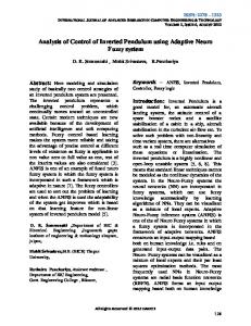
Figure 1: Double Inverted pendulum on a cart θ0 θ00 θ1 θ10 θ2 θ20

Cart position Cart velocity Angle of the lower pendulum Angular velocity of the lower pendulum Angle of the upper pendulum Angular velocity of the upper pendulum

The Lagrange Equations of Motion are defined as   d dL dL =Q − dt dφ0 dθ

(1)

where Q the vector of external forces acting on the system. These equations lead to the system ([6]): D(θ)θ00 + C(θ, θ0 )θ0 + G(θ) = Hu

(2)

where 

 d1 d2 cosθ1 d3 cosθ2 d4 d5 cos(θ1 − θ2 ) D(θ) = d2 cosθ1 d3 cosθ2 d5 cos(θ1 − θ2 ) d6   0 0 −d2 sin(θ1 )θ1 −d3 sin(θ2 )θ20 0 d5 sin(θ1 − θ2 )θ20  C(θ, θ0 ) = 0 0 0 −d5 sin(θ1 − θ2 )θ1 0   0 G(θ) = −f1 sinθ1  −f2 sinθ2   1 H = 0 0

(3)

(4)

(5)

(6)

with d1 = m0 + m1 + m2 d2 = (m1 /2 + m2 )L1 d3 = m2 L2 /2

(7)

d4 = (m1 /3 + m2 )L21

d5 = m2 L1 L2 /2

(8)

f1 = (m1 /2 + m2 )L1 g

f2 = m2 L2 g/2 2

d6 = m2 L22 /3

(9)

and g is the gravitational acceleration. The above equations describe the system’s motion and are clearly nonlinear. The linearization of these equations around the equilibrium (θ0 , θ1 , θ2 , θ00 , θ10 , θ20 ) = (0, ..., 0)

(10)

leads to the following state space system

where

 A=

and the state vector is

x0 (t) = Ax(t) + Bu(t)

(11)

y(t) = x(t)

(12)

0

D(0)−1 dG(0) dθ

I 0

 B=

0 D(0)−1 H

 (13)

  θ0 θ1      θ2  θ  x= = 0 θ00  θ  0 θ1  θ20

If we compute the above matrices for the following L1 = 0.5m, L2 = 0.75m we end up with  0 0 0 1 0 0 0 0  0 0 0 0 A= 0 −7.4920 0.7985 0  0 74.9266 −33.7147 0 0 −59.9373 52.1208 0

3



(14)

data: m0 = 1.5kg, m1 = 0.5kg, m2 = 0.75g, 0 1 0 0 0 0

 0 0  1  0  0 0

 0   0     0   B=  −0.6070    1.4984  −0.2839 

(15)

Linear Quadratic Regulator solution (LQR)

Now that the system is defined, our next aim is to define a cost function depending on the position and the input and minimize it with respect to these parameters. Let J = xT Qx + uT Ru where Q, R are weight matrices for each parameter. According to [6], we will define Q = diag(5, 50, 50, 20, 700, 700)

R=1

although of course other cost functions can be defined, depending on the capabilities of the mechanical system used in a real life simulation. The input that is used is of the form u = −Kx, where K is the state feedback matrix and is the solution of the Riccati equation. This matrix can be obtained from Matlab using the command k=lqr(sys,Q,R), where sys is the above state space system, to which we have set y = x so that the states are equal to the outputs. The matrix K is
k = −2.2361 499.6181 −578.2160 −8.2155 19.1832 −88.4892 (16) so after the feedback is applied, the new system’s matrix is  0 0 0 1  0 0 0 0   0 0 0 0 A − Bk =   −1.357 295.8 −350.2 −4.987   3.351 −673.7 832.7 12.31 −0.6348 81.9 −112 −2.332 3

0 1 0 11.64 −28.74 5.446

 0 0   1   −53.72  132.6  −25.12

(17)

Consider the response for initial conditions     0 θ0 θ1   10      θ2  −10   0 =  θ0   0    0  θ1   0  0 θ20

(18)

that is, for a relatively small deflections from the equilibrium. It should be noted here that although we refer to the deflection angles in degrees, in matlab, they should be inputed in radians, as can be seen from the matlab code at the end. The six states can be seen in Figure 2.

Figure 2: Lqr solution for initial conditions (18) For larger deflections towards the same direction     θ0 0 θ1  20     θ2  20  0 =   θ0   0   0   θ1   0  θ20 0

(19)

the states can be seen in Figure 3. Again we can see that the system can be balanced, although the cart is stabilized far from the point 0, to which it returns to with a very low pace.

4

Figure 3: Lqr solution for initial conditions (19)

4

Simulation Code for LQR

% Define the parameters m0=1.5 ; m1 =0.5 ; m2 =0.75 ; L1 =0.5 ; L2 =0.75 ; dt= 0.02 ; Q =diag([5 50 50 700 700 700]); % One can also try the following % Q =diag([700, 0, 0, 0, 0, 0]) % Q=diag([110 110 110 0 0 0]) R =1; Nh =40; g=10; % Define the system matrices d0=[m0 + m1 + m2, (m1/2 + m2)*L1, (m2*L2)/2;(m1/2 + m2)*L1, ... (m1/3 + m2)*L1ˆ2,(m2*L1*L2)/2;(m2*L2)/2,(m2*L1*L2)/2,(m2*L2ˆ2)/3]; g=[0,0,0;0,-(m1/2 + m2)*L1*10,0;0,0,-(m2*L2*g)/2];

% Define the State Space System a=[zeros(3),eye(3);-inv(d0)*dg,zeros(3)]; b=[zeros(3,1);inv(d0)*[1;0;0]]; c=eye(6); sys=ss(a,b,eye(6),0) % Compute the feedback k k=lqr(sys,Q,R) % Define the new system sysnew=ss(a-b*k,b,c,0)

5

% Simulate the system for initial conditions [y,t,x]=initial(sysnew,[0;deg2rad(10);-deg2rad(10);0;0;0],7); % [y,t,x]=initial(sysnew,[0;deg2rad(20);deg2rad(20);0;0;0],10); % Convert from rad to deg y(:,2:3)=rad2deg(y(:,2:3)); y(:,5:6)=rad2deg(y(:,5:6)); % Plot the data close all for i=1:1:6 subplot(2,3,i) plot(t,y(:,i)) grid end

5

Model predictive control using Laguerre functions

The basic idea of solving a problem through model predictive control is to find a way to construct the optimal control trajectory. The control sequence will be computed for a specific time interval called Control Horizon Nc , and it will determine the progress of the system for a longer time interval called the Prediction Horizon [13]. The first step in this procedure is the discretization of the model. Using zero order hold with sampling period T = 0.002s, the discrete time model is

with

 1 0  0 Ad =  0  0 0

0 1.0001 −0.0001 −0.0150 0.1499 −0.1199

x(k + 1) = Ad x(k) + Bd u(k)

(20)

y(k) = x(k)

(21)

0 0.0020 −0.0001 0 1.0001 0 0.0016 1 −0.0674 0 0.1042 0

0 0.0020 0 0 1.0001 −0.0001

 0  0  0.0020    0  −0.0001 1.0001

 0   0     0  Bd =   0.0012    −0.0030 0.0006

the next step is to construct the augmented model, which is        ∆x(k + 1) Ad 0 ∆x(k) Bd = + ∆u(k) y(k + 1) IAd I y(k) IBd | {z } | {z } Aaug

y(k) = 0



(22)

(23)

Baug

 
∆x(k) I y(k)

(24)

where C = I, since we want to have y = x. Our aim now is to compute the control sequence ∆u(k),using Laguerre functions [13].Laguerre functions are used in order to compute the optimal control input ∆u(k), which is then applied to the system through state feedback ∆u(k) = −Kmpc xaug (k) (25) where Kmpc = L(0)T Ω−1 Ψ

6

(26)

with L(0)T =

p 1 − a2 1

a2

−a

−a3

... (−1)Nc −1 aNc −1




(27)

Np

Ω=

X

φ(m)Qφ(m)T + RL

(28)

m=1 Np X

Ψ= φ(m)T =

φ(m)QAm aug

(29)

m=1 m−1 X

Am−i−1 Baug L(i)T aug

(30)

i=0

L(i) = l1 (i) · · ·

lNc (i)


T

(31)

where l(i) are the Laguerre functions, a ∈ (0, 1) and Q, RL are the regulator matrices, Q is a 12 by 12 diagonal matrix and R is also a diagonal Nc × Nc matrix. Let the parameters be
a = 0.4 Q = diag( 11 11 11 0 0 0 11 11 11 0 0 0 ) RL = 0 (32) and the control and prediction horizons N p = 1000

N c = 200

(33)

The feedback matrix Kmpc is computed to be Kmpc = L(0)T Ω−1 Ψ = = 37.7155

−283.1523

453.8848

33.5609

4.5332

71.5215

0.0422

0.0205

0.0187

0

0


0 (34)

With this feedback, the system becomes xaug (k + 1) = (Aaug − Baug Kmpc )xaug (k) + Baug ∆u(k)

(35)

y(k) = Caug xaug (k)

(36)

From the above system we can recreate the original 6 by 6 pendulum system, since C = I. The original system is just the 6 by 6 block part of (Aaug − Baug Kmpc ) and the first 6 lines of Baug . The response for initial conditions     θ0 0 θ1  5     θ2  5  0 =   (37) θ0  0  0   θ1  0 θ20 0 can be seen in Figure 4. For larger deflections     θ0 0 θ1   15      θ2  −15  0 =   θ0   0   0   θ1   0  θ20 0

(38)

the response can be seen in Figure 5. Here we can observe that the lower pendulum has for a time period a large anglar velocity, which of course os undesired. 7

Figure 4: Mpc response for initial conditions (37)

Figure 5: Mpc response for initial conditions (38)

6

Simulation Code for MPC

%% Discretize and get Augmented System format long

8

sysd=c2d(sys,0.002,'zoh'); [ad,bd,cd,dd]=ssdata(sysd); % One can also try: % ad=expm(a*0.02) % bd=b*0.02; sysd=ss(ad,bd,cd,dd); ad comp=[ad, zeros(6);cd*ad, eye(6)]; bd comp=[bd;cd*bd]; cd comp=[zeros(6),eye(6)]; augmented=ss(ad comp,bd comp,cd comp,0,0.002); %% Design MPC Using Laguerre Functions a=0.4; beta=sqrt(1-aˆ2); Np=1000; Nc=200; Q =diag([11 11 11 0 0 0 11 11 11 0 0 0]); % Create Laguerre Matrix [A1,L0T]=lagd(a,Nc); clear L L(:,1)=L0T; for kk=2:Np; L(:,kk)=A1*L(:,kk-1); end %% Define Psi and Omega psi=0; omega=0; for i=1:Np f=0; lag=[]; for j=0:i-1 f=f+ad compˆ(i-1-j)*bd comp *L(:,j+1)'; end psi=psi+f'*Q*ad compˆi; omega=omega+f'*Q*f; end %% Define Augmented System with Feedback finalsys=ss(ad comp-bd comp *L0T'*pinv(omega)*psi,bd comp,cd comp,0,0.002); %% Define Original System with Feedback am=(ad comp-bd comp *L0T'*pinv(omega)*psi); %A after feedback final=ss(am(1:6,1:6),bd comp(1:6),eye(6),0,0.002); % Plot for Chosen Initial Conditions [y,t,x]=initial(final,[0;deg2rad(5);deg2rad(5);0;0;0;],7); %[y,t,x]=initial(final,[0;deg2rad(15);deg2rad(-15);0;0;0;],10); y(:,2:3)=rad2deg(y(:,2:3)); y(:,5:6)=rad2deg(y(:,5:6)); for i=1:1:6 subplot(2,3,i) plot(t,y(:,i)) grid end

In the above code we made use of the function lagd which is taken from [13]. function [A,L0]=lagd(a,N) v(1,1)=a; L0(1,1)=1; for k=2:N v(k,1)=(-a).ˆ(k-2)*(1-a*a); L0(k,1)=(-a).ˆ(k-1);

9

end L0=sqrt((1-a*a))*L0; A(:,1)=v; for i=2:N A(:,i)=[zeros(i-1,1);v(1:N-i+1,1)]; end

References [1] Nise, N. S. (2015). Control Systems Engineering (7th Edition). John Wiley and Sons. [2] Franklin, G. F., J. D. Powell, and A. Emami-Naeini. Feedback control of dynamics systems. AddisonWesley, Reading, MA 1994. [3] Golnaraghi, Farid, and B. C. Kuo. Automatic control systems, 9th ed. Wiley, 2009. [4] Tobias Brull, Course: Systems and control theory, Lecture Notes: Equations of motion for an inverted double pendulum on a cart (in generalized coordinates). Institute of Mathematics, Un. of Berlin. [5] Pathompong Jaiwat, and Toshiyuki Ohtsuka, Real-Time Swing-up of Double Inverted Pendulum by Nonlinear Model Predictive Control. 5th International Symposium on Advanced Control of Industrial Processes, May 28-30, 2014, Hiroshima, JAPAN. [6] Alexander Bogdanov, Optimal Control of a Double Inverted Pendulum on a Cart. Technical Report CSE-04-006, 2004. [7] S. Jadlovsk´ a and J. Sarnovsk´ y, Classical Double Inverted Pendulum - a Complex Overview of a System. IEEE 10th International Symposium on Applied Machine Intelligence and Informatics (SAMI), 2012. [8] S. Jadlovsk´ a, A. Jadlovsk´ a, Inverted pendula simulation and modeling - a generalized approach, 9th International Conference PROCESS CONTROL, June 7 - 10, 2010, Kouty nad Desnou, Czech Republic. [9] Qi Qian, Deng Dongmei, Liu Feng and Tang Yongchuan, Stabilization of the Double Inverted Pendulum Based on Discrete-time Model Predictive Control, IEEE International Conference on Automation and Logistics, Chongqing, China, August 2011. [10] T. Henmi, M. Deng, A. Inoue, N. Ueki, and Y. Hirashima,Swing-up Control of a Serial Double Inverted Pendulum. Proceedings of the 2004 American Control Conference, Boston, Massachusetts June 30 - July 2, 2004. [11] M. R. Nalavade, M. J. Bhagat, V. V. Patil, Balancing Double Inverted Pendulum on A cart by Linearization Technique. International Journal of Recent Technology and Engineering (IJRTE) ISSN: 2277-3878, Volume-3, Issue-1, March 2014. [12] M. Gulan, S. Michal, and R. Boris. Achieving an equilibrium position of pendubot via swing-up and stabilizing model predictive control. Journal of Electrical Engineering 65.6 (2015): 356-363. [13] L. Wang, Model Predictive Control System Design and Implementation Using MATLAB. Springer, 2009. [14] Moysis, L., Tsiaousis, M., Charalampidis, N., Eliadou, M., & Kafetzis, I. An Introduction to Control Theory Applications with Matlab. 2015. DOI: 10.13140/RG.2.1.3926.8243

10