Bandwidth-Constrained MAP Estimation for Wireless Sensor Networks

Bandwidth-Constrained MAP Estimation for Wireless Sensor Networks S. Faisal Ali Shah, Alejandro Ribeiro and Georgios B. Giannakis Dept. of ECE, University of Minnesota 200 Union Street S.E., Minneapolis, MN 55455

Work in this paper was prepared through collaborative participation in the Communications and Networks Consortium sponsored by the U. S. Army Research Laboratory under the Collaborative Technology Alliance Program, Cooperative Agreement DAAD19-01-2-0011. The U. S. Government is authorized to reproduce and distribute reprints for Government purposes notwithstanding any copyright notation thereon. Email at (sfaisal, aribeiro, georgios)@ece.umn.edu

1­4244­0132­1/05/$20.00 ©2005 IEEE

Fig. 1.

Transducer

Quantizer/ Encoder

.. .

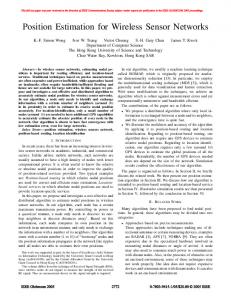
Characterized by small low-cost, low-power devices equipped with limited sensing, computational and communication capabilities, wireless sensor networks (WSNs) are well motivated for environmental monitoring, industrial instrumentation and surveillance applications [7]. The distributed topology of these networks along with their limited power budget and communication resources gave rise to the area of collaborative signal and information processing [3]. Bandwidth-constrained distributed estimation arises when deploying a WSN for monitoring, in which case the estimation of certain parameters of interest necessitates collection of different sensor estimates. As sensor observations have to be quantized, WSN-based parameter estimators must rely on (perhaps severely) quantized observations [4], [5]. Interestingly, it has been shown in [6] that when the noise variance is comparable to the parameter’s dynamic range, even quantization to a single bit per observation leads to a small penalty in estimation variance when comparing maximum likelihood (ML) estimators based on quantized (binary) versus original (analog-amplitude) observations. A characteristic common to all these works is the assumption that some prior information is available, at least to bound the range of possible parameter values. This suggests naturally, a connection with Bayesian estimation. Building on this observation, the present paper addresses the problem of maximum a posteriori (MAP) estimation based on binary observations, and shows that the graceful

Physical Phenomenon /Process

.. .

I. I NTRODUCTION

BW/Power Constrained Links

Sensor nodes

.. .

Abstract— We deal with distributed parameter estimation algorithms for use in wireless sensor networks (WSNs) with a fusion center when only quantized observations are available due to power/bandwidth constraints. The main goal of the paper is to design efficient estimators when the parameter can be modelled as random with a priori information. In particular, we develop maximum a posteriori (MAP) estimators for distributed parameter estimation and formulate the problem under different scenarios. We show that the pertinent objective function is concave and hence, the corresponding MAP estimator can be obtained efficiently through simple numerical maximization algorithms.

Estimator (Fusion Center)

Block diagram of wireless sensor network

performance degradation of ML estimators extends to their MAP counterparts. Moreover, we establish that while MAP estimators cannot be expressed in closed form, they are found as the maximum of a concave function; thus ensuring the convergence of fast descent algorithms e.g., Newton’s method. II. P ROBLEM F ORMULATION Consider a physical phenomenon characterized by a set of P parameters that we lump in vector form as θ := [θ1 , . . . , θP ]T . From available a priori knowledge, θ is modelled as a random vector parameter with prior probability density function (pdf) pθ (θ) and mean E(θ) = µθ . For measuring θ, we deploy a WSN composed of N sensors −1 {Sn }N n=0 , with each sensor observing θ through a linear transformation x(n) = Hθ + w(n), (1) where x(n) := [x1 (n), . . . , xK (n)]T ∈ RK is the measurement vector at sensor Sn , w(n) ∈ RK is zero-mean additive noise with pdf pw (w) and the matrix H ∈ RK×P . We denote the vector formed by concatenating all the observa−1 tions {x(n)}N n=0 of N sensors as x0:N −1 . For simplicity of exposition, we assume that H and pw (w) are constant across sensors, and we also assume that w(n1 ) is independent of w(n2 ) for n1 = n2 . A clairvoyant (CV) benchmark for estimators based on binary observations corresponds to having all analog-amplitude observations x0:N −1 be available at the fusion center. In this case, a possible approach to estimate θ is the MAP estimator [2] θˆCV

=

arg maxθ {p[θ|x0:N −1 ]} ,

(2)

where p[θ|x0:N −1 ] is the conditional pdf of θ given x0:N −1 . As discussed earlier, power and bandwidth constraints, dictate the need of a quantizer mapping the analog-amplitude observations x(n) to a finite set:

215

b(n) := q(x(n)),

with

q : RK → {−1, 1}K ,

(3)

with b(n) = [b1 (n), . . . , bK (n)]T a K-component binary message. Note that implicit to (3) is the fact that we are restricting the sensors to transmit one bit per scalar observation. Similar to x0:N −1 , we define the binary observation of N sensors as b0:N −1 . The problem addressed in this paper is the MAP estimation of θ based on the binary messages b0:N −1 , where the MAP estimator is defined as [2] θˆMAP

= arg maxθ {p[θ | b0:N −1 ]}

(4)

= arg maxθ {ln p[b0:N −1 |θ] + ln pθ (θ)} , with p[θ | b0:N −1 ] and p[b0:N −1 |θ] are the conditional pdfs of θ given b0:N −1 and of b0:N −1 given θ, respectively. Note that to obtain the second equality in (4) we used Bayes’ rule, the monotonicity of the logarithm and eliminated a normalizing constant that does not depend on θ. The goals of this paper are to: i) derive quantization functions q(x(n)); ii) establish that in many cases of interest θˆMAP in (4) can be found as the maximum of a concave function; and iii) show that the estimation variance of θˆMAP in (4) based on binary observations comes close to the estimation variance of θˆCV in (2) based on analog-amplitude observations. III. MAP E STIMATOR - S CALAR PARAMETERS The MAP formulation allows us to tackle parameter estimation problems in different scenarios. First simple situation is when the parameter θ ↔ θ and the observations x(n) ↔ x(n) are scalar. In this case, we define the message as b(n) := sgn[x(n) − hµθ ]

(5)

where the function sgn(·) observes the sign of its argument. The estimator θˆMAP in (4) can then be written in terms of the prior pdf pθ (θ) and the cumulative distribution function (CDF) of the noise and can be found with robust numerical algorithms as asserted by the following proposition. Proposition 1 Consider a random scalar parameter θ with prior distribution pθ (θ), an observation model as in (1), and binary messages b0:N −1 defined as in (5). Then, (a) if Fw (w) denotes the CDF of the noise variables w(n) the MAP estimator of θ given b0:N −1 is
N −1   ˆ ln Fw [hb(n)(θ−µθ )]+ln pθ (θ) θMAP = arg max θ

n=0

:= arg maxθ [L(θ)]

(6)

and; (b) if Fw (·) and pθ (·) are log-concave functions [1, p. 104], then L(θ) is a concave function of θ. Proof: Writing (4) for scalar parameter θ θˆMAP = arg maxθ ln p(θ|b0:N −1 ) = arg maxθ {ln Pr[b0:N −1 | θ] + ln p(θ)} ,

(7)

where we ignored the term containing Pr(b0:N −1 ) as it is independent of θ. Making use of the independence among the obN −1 servations, we can write Pr[b0:N −1 |θ] = n=0 Pr[b(n) | θ].

The value of Pr[b(n)|θ] can be obtained by explicit enumeration: Pr[b(n) = 1|θ] = Pr[w > h(µθ − θ)|θ] =

Fw [h(θ − µθ )]

Pr[b(n) = −1|θ] = Pr[w < h(µθ − θ)|θ] = Fw [h(µθ − θ)] . Combining the above two cases, we can write Pr[b(n)|θ] = Fw [hb(n)(θ − µθ )] .

(8)

Substituting (8) into (7) the result in (6) follows. The claim in Proposition 1-[b] follows from the fact that the sum of concave functions is also concave. The value of Proposition 1 is not as much in giving an expression for θˆMAP (Proposition 1-[a]) as in establishing that the function L(θ) is concave (Proposition 1-[b]). The latter assures efficient numerical implementation of our algorithm as discussed in the following remark. Remark 1 The numerical search needed to obtain θˆMAP could be challenged either by the multimodal nature of L(θ) or by numerical ill-conditioning caused by e.g., saddle points. But when the log-concavity conditions in Proposition 1-[b] are satisfied, computationally efficient search algorithms like e.g. Newton’s method are guaranteed to converge to the global maximum [1, Chap. 2]. A special case of a log-concave pdf is the Gaussian one. Consequently, in the frequently encountered case of a √ 2 2 Gaussian prior pθ (θ) = [1/( 2πσ√ θ )] exp[−(θ − µθ ) /(2σθ )] 2 2 and Gaussian noise pw (w) = [1/( 2πσw )] exp[−w /(2σw )] the MAP estimator can be expressed as    2 N −1 hb(n)(µθ −θ) θ) − (θ−µ , θˆMAP = arg maxθ n=0 ln Q σw 2σθ2 (9)

∞ √ where Q(x) := x (1/ 2π) exp[−u2 /2]du is the Gaussian tail function. Moreover, descent methods e.g., Newton’s algorithm are guaranteed to converge to the global maximum. Other log-concave pdfs are the uniform distribution in a convex set and the members of the generalized Gaussian family. IV. MAP E STIMATOR - VECTOR PARAMETERS Results in Section III can be extended to cover the general vector parameter - vector observation model in (1). Start by considering the case of white Gaussian noise; i.e., 2 I. In this case, we write H := E[w(n)wT (n)] = σw T [h1 , . . . , hK ] and define the components of the message b(n) as bk (n) := sgn[xk (n) − hTk µθ ] , (10) for k ∈ [1, K]. The resemblance with the problem of Section III is clear and not surprisingly the following proposition holds true. Proposition 2 Consider a vector parameter θ, with logconcave prior distribution pθ (θ); an observation model as in (1) with pw (w) white Gaussian with variance 2 E[w(n)wT (n)] = σw I; and binary messages b0:N −1 as

216

in (10). Then, if we define the per sensor likelihood Ln (θ) as  K  bk (n)hTk [µθ − θ] , (11) ln Q Ln (θ) = σw

On the other hand, note that uk1 (n) and uk2 (n) are independent for k1 = k2 . Indeed, since uk (n) is normally distributed it suffices to prove that uk1 (n) and uk2 (n) are uncorrelated: E[uk1 (n)uk2 (n)] = vkT1 (n)E[w(n)wT (n)]vk2 (n)

k=1

= vkT1 (n)C(n)vk2 (n)

we have that: (a) The MAP estimator of θ based on b0:N −1 is given by
N −1   ˆ Ln (θ) + ln[pθ (θ)] θMAP = arg max

= σk21 (n)δ(k1 − k2 );

θ

n=0

:= arg maxθ L(θ).

(12)

(b) The likelihood L(θ) is a concave function of θ. Let us note that the multivariate Gaussian belongs to the log-concave class of pdfs. Indeed, if θ has a Gaussian prior distribution with covariance matrix E[θθ T ] = Cθ then 1 T ln[pθ (θ)] = −C − (θ−µθ ) C−1 θ (θ−µθ ) , 2

(13)

with C := 12 ln[(2π)P det(Cθ )]. The expression in (13) is a quadratic expression on θ which is concave for positive semidefinite Cθ . Proposition 2 establishes that at least for white Gaussian noise the comments in Remark 1 also hold true for vector parameters and observations. In the coming section we show that the same result can be obtained for colored noise. A. Colored Gaussian Noise Consider again the model in (1) with w(n) colored Gaussian with covariance matrix E[w(n)wT (n)] := C(n) at sensor Sn . In this case the components of the observation x(n) are not independent; hence, the components of b(n) are not and the conditional probabilities in (4) are difficult to obtain in general. Nonetheless, there is a particular definition of b(n) that results in independent components. Consider the eigenvector decomposition of C(n), 2 (n)]VT (n), C(n) = V(n)diag[σ12 (n), . . . , σK

where are the eigenvalues of C(n) and V(n) := [v1 (n) . . . vK (n)] is the matrix of eigenvectors such that viT (n)C(n)vj (n) = σi2 (n)δij . If we define the k th component of bk (n) as

 bk (n) := sgn vkT (n){x(n) − Hµθ } , (15) the resultant binary observations are independent when θ is given as we assert in the following lemma: Lemma 1 Consider the model in (1) with w(n) Gaussian with covariance matrix E[w(n)wT (n)] := C(n). Then, binary observations defined as in (15) are independent for k1 = k2 : Pr{bk1 (n), bk2 (n)|θ} = Pr{bk1 (n)|θ} Pr{bk2 (n)|θ}

Lemma 1 follows because bk1 (n) and bk2 (n) are functions of the independent random variables uk1 (n) and uk2 (n) [c.f. (16) and (18)]. The independence of the binary observations dictates that the per-sensor log-likelihood can be written as  K  bk (n)vkT H [µθ − θ] . (19) ln Q Ln (θ) = σk (n) k=1

From where a proposition analogous to Proposition 2 follows readily. Proposition 3 Consider the setting of Proposition 2 with pw (w) colored Gaussian with covariance matrix E[w(n)wT (n)] := C(n) at sensor Sn ; binary messages b0:N −1 as in (15); and per-sensor log-likelihood Ln (θ) as in (19). Then, results [a] and [b] of Proposition 2 hold true. Propositions 1-3 establish that for many pragmatic signal models MAP estimation from binary observations can be posed as a convex optimization problem with virtues summarized in Remark 1. V. M EAN -S QUARE E RROR (MSE) A NALYSIS In this section, we study the increase in mean-square error (MSE) when binary observations are used in lieu of the analogamplitude observations. For estimation of random parameters, bounds on the MSE can be obtained by computing the pertinent Fisher Information Matrix (FIM) J that we write as the sum of two parts [8, p. 84]:

(14)

{σk2 (n)}K k=1

(16)

Proof: Define uk (n) := vkT (n)w(n) and note that the distribution of bk (n) is given by [c.f (1), (15)] Pr{bk (n) = ±1|θ} = Pr{uk (n) ≷ vkT (n)H(θ − µθ )}. (17)

(18)

J = JD + JP ,

(20)

where JD represents information obtained from the data, and JP captures a priori information. The MSE of the ith component of θ is bounded by the ith diagonal element of J, 

(21) MSE(θˆi ) ≥ J−1 ii . Also, note that for any FIM, [J−1 ]ii ≥ 1/[J]ii [2]. This property yields a different bound on MSE(θˆi ), MSE(θˆi ) ≥

1 , [ J ]ii

(22)

which is easier to compute although not tight in general. The following proposition states a bound (exact value) on [J]ii when binary (analog-amplitude) observations are used. Proposition 4 Consider the signal model in (1) with w(n) 2 I white Gaussian with covariance matrix E[w(n)wT (n)] = σw T and Gaussian prior distribution with covariance E[θθ ] = Cθ . Write (1) componentwise as x(n) is xk (n) = hTk θ +

217

wk (n). Then, the ith diagonal element of the FIM J in (20) satisfies: (a) when binary observations as in (10) are used, [ J ]ii ≥

MSE of θ1 Analog MAP Theoretical Simulation −1

MSE

10

K 

h2ki 2N   + C−1 , (23) θ ii πσw T 2 +h C h σw k=1 k θ k

−2

10

2

10 Number of sensors (N) MSE of θ2

(b) when analog-amplitude observations are used,

Analog MAP Theoretical Simulation −1

10

(24)

MSE

K 

N  2 hki + C−1 . [JCV ]ii = 2 θ ii σw k=1

Proof: See Appendix A. For the clairvoyant FIM, JCV , the bound derived above is essentially the same as the one obtained for MMSE estimators in [2]. Indeed, the MSE for the Gaussian prior - Gaussian noise considered in Proposition 4 is
 −1  1 T −1 ˆ MSE(θi ) = H H + Cθ . (25) 2 σw

−2

10

2

10 Number of sensors (N)

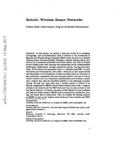
Fig. 2. [cos ψ

MSE of MAP estimator vs. number of sensors (γ = 0.3; h = sin ψ] with ψ ∈ [−π, π]) MSE of θ1 Analog MAP Theoretical

ii

MSE

Comparing (25) with (21), we see that the term inside the parenthesis in (25) is the FIM in (24). For the bound when binary observations are used, corroborating simulations in Section VI prove that it is actually tight. Consequently, it provides a good theoretical means to characterize the performance of estimators based on binary observations.

−2

10

[JCV ]ii MSE(θˆi ) ≈ . Li := [ J ]ii MSE(θˆi,CV )

(26)

For large N , the second terms in (23) and (24) can be neglected and the information loss can be approximated as:  π hT Cθ h π Li ≈ 1+ := 1 + γ, (27) 2 2 σw 2 2 where we defined γ := hT Cθ h/σw which is the average signal to noise ratio (SNR) of the observations x(n). Note that as γ → 0 the information loss Li → π/2, corroborating results in [6] for deterministic parameter estimation. In any event, we stress the remarkable fact that for low to medium SNR γ, the average information loss Li is a small factor.

VI. N UMERICAL R ESULTS Consider using the MAP estimator in (12) to estimate a two-dimensional vector parameter. The random vector θ := [θ1 θ2 ]T is assumed to have zero mean and diagonal covariance matrix Cθ = σθ2 I. Our goal is to find the MSE of θˆ as E[(θ − ˆ 2 ] through simulations and compare it with the analytical θ) results of Section V. We first study the effect of the number of sensors N on the MSE with results shown in Fig. 2. Simulated MSE values are scattered around analytical corroborating our approximate

−1

0

10

10 SNR (γ) MSE of θ2

Analog MAP Theoretical −1

MSE

Remark 2 As a figure of merit, consider the MSEs when estimating θi from a set of quantized observations b0:N −1 and when using analog-amplitude observations x0:N −1 . We define the average information loss Li as

Simulation

−1

10

10

Simulation

−2

10

−1

0

10

10 SNR (γ)

Fig. 3. MSE of MAP estimator vs. SNR (N = 100; h = [cos ψ with ψ ∈ [−π, π])

sin ψ]

analysis. We also compare the results with the analog MAP estimator finding that the performance loss in terms of increased MSE is relatively small, consistent with the comments in Remark 2. 2 For fixed N , results for different values of SNR γ := σθ2 /σw are shown in Fig. 3. Note that different from the MAP based on analog observations, the MSE of the MAP based on binary observations increases with γ (it is constant for the former). Figs. 2 and 3 show that the simulation results follow the analytical results closely. VII. C ONCLUSIONS We investigated distributed maximum a posteriori (MAP) estimation of random parameters using wireless sensor networks (WSN) with severely quantized observations. For different pragmatic signal scenarios considered, we established that the MAP estimators can be obtained as the maximum of concave functions, thus ensuring convergence of e.g., interior point methods. We also compared the MSE performance of our estimators based on severely quantized data with estimators based on analog-amplitude observations. While the MSE performance penalty increases with the observation signal

218

to noise ratio (SNR) we showed that, quite surprisingly, the MSE increase is rather small. Future research directions include consideration of estimation based on quantized – nonnecessarily binary – data and application of MAP to state estimation of dynamic stochastic processes based on quantized data. A PPENDIX A. Proof of Proposition 3 From (20), the ith diagonal element of FIM has two parts: [ J ]ii = [JD ]ii + [JP ]ii and each part is defined as :  2  ∂ ln p [b0:N −1 |θ] (28) [JD ]ii := −Eθ,b ∂θi2  2  ∂ ln pθ (θ) [JP ]ii := −Eθ,b . (29) ∂θi2 Note that the expectation in (28) and (29) is joint with  respect  to θ and b. It can be expressed as: Eθ,b [.] = Eθ Eb|θ [.] . −1 Assuming independence among the sensors {Sn }N n=0 and K each observation {bk (n)}k=1 of sensor Sn , we can write the probability in (28) as: ln p [b0:N −1 |θ] =

N −1  K 

Since the prior distribution of θ is Gaussian, we reach  ∞ K 2N (det Cθ )−1/2  2 [JD ]ii ≥ h e−Gk (θ) dθ, ki 2 (2π)K/2 πσw −∞ k=1

where the exponent in the integrand is given by 1 1 Gk (θ) = [hTk (θ − µθ )]2 + (θ − µθ )T C−1 θ (θ − µθ ) 2 2σw 2

 1 = αT gk gkT + I α 2 −1/2

:= F(θ), bk (n)hT k [µθ −θ]

−∞

(30)

k=1

where we have used the fact that Eb|θ [bk (n)] = 2qk − 1. Now, differentiating qk wrt to θi , we find (33)

Using the chernoff bound and (33), eq. (32) becomes
N −1 K    h2 e−[hTk (µθ −θ)]2 /σw2 1 ki [JD ]ii ≥ Eθ T 2 2 2 2πσw (1/4)e−[hk (µθ −θ)] /2σw n=0 k=1

K   T 2 2 2N  2 hki Eθ e−[hk (µθ −θ)] /2σw ≥ 2 πσw k=1  ∞ K T 2 2 2N  2 hki e−[hk (θ−µθ )] /2σw pθ (θ)dθ. ≥ 2 πσw −∞ k=1

1/2

det(gk gkT + I)−1/2 .

The determinant can be evaluated as a product of the eigen−2 T 1/2 values of gk gkT + I. Since gk gkT /(σw hk Cθ hk ) is an idempotent matrix with eigenvalues 1 or 0, the eigenvalues −2 T 1/2 of gk gkT are σw hk Cθ hk or 0. Hence, the eigenvalues of −2 T 1/2 hk Cθ hk or 1. Thus, det(gk gkT + gk gkT + I will be 1 + σw −2 T I) = 1 + σw hk Cθ hk . This finally leads to [JD ]ii ≥

since w(n) is Gaussian. with p[bk (n)|θ] = Q σw To facilitate the analysis, we define an observation independent   T h [µ −θ] quantity qk := Q k σwθ . Since bk (n) ∈ {±1} and Q(−a) = 1 − Q(a), an equivalent form of the log-likelihood in (30) is given by  K  N −1  1 + bk (n) 1 − bk (n) F(θ) = ln qk + ln{1 − qk } . 2 2 n=0 k=1 (31) Differentiating (31) twice with respect to (wrt) θi and evaluating the expectation Eb|θ , we obtain
N −1 K  2   ∂qk 1 , (32) [JD ]ii = Eθ qk (1 − qk ) ∂θi n=0

T 2 2 ∂qk 1 = −√ e−[hk (µθ −θ)] /2σw hki . ∂θi 2πσw

−∞

= (2π)K/2 |det Cθ |

ln p[bk (n)|θ]



1/2

−1 where we define α := Cθ (θ−µθ ) and gk := σw Cθ hk . With this, the integral in (34) becomes  ∞  ∞ T T 1 1/2 e−Gk (θ) dθ = e− 2 α (gk gk +I)α |det Cθ | dα

n=0 k=1



(34)

K 2N  h2ki  . πσw 2 + hT C h σw k=1 k θ k

(35)

Similarly, the FIM for the a priori information is given by JP = C−1 θ .

(36)

From (35) and (36), we find the bound on the ith diagonal element of FIM as given by (23). For the Clairvoyant estimator, the conditional probability in (28) is Gaussian such that ln p [x0:N −1 | θ] = −

N −1 K 2 1   xk (n) − hTk θ . 2 2σw n=0

(37)

k=1

Differentiating (37) twice wrt to θi and computing the joint expectation wrt b and θ we get the result as in (24). R EFERENCES [1] S. Boyd and L. Vandenberghe, Convex Optimization. Cambridge University Press, 2004. [2] S. M. Kay, Fundamentals of Statistical Signal Processing - Estimation Theory. Prentice Hall, 1993. [3] S. Kumar, F. Zhao, and D. Shepherd, “Collaborative signal and information processing in microsensor networks,” IEEE Signal Processing Magazine, vol. 19, pp. 13–14, March 2002. [4] Z.-Q. Luo, “An isotropic universal decentralized estimation scheme for a bandwidth constrained ad hoc sensor network,” IEEE Journal on Selected Areas in Communications, vol. 23, pp. 735–744, April 2005. [5] H. Papadopoulos, G. Wornell, and A. Oppenheim, “Sequential signal encoding from noisy measurements using quantizers with dynamic bias control,” IEEE Transactions on Information Theory, vol. 47, pp. 978– 1002, 2001. [6] A. Ribeiro and G. B. Giannakis, “Bandwidth-Constrained Distributed Estimation for Wireless Sensor Networks, Part II: Unknown pdf,” IEEE Transactions on Signal Processing, 2006 (to appear). [7] S. Servetto, R. Knopp, A. Ephremides, S. Verdu, S. Wicker, and L. Cimini, “Guest Editorial: Fundamental performance limits of wireless sensor networks,” IEEE Journal on Selected Areas on Communications, vol. 22, pp. 961–965, August 2004. [8] H. L. V. Trees, Detection, Estimation, and Modulation Theory. J. Wiley and Sons Inc., first ed., 1968.

219