The International Archives of the Photogrammetry, Remote Sensing and Spatial Information Sciences, Volume XLI-B7, 2016 XXIII ISPRS Congress, 12–19 July 2016, Prague, Czech Republic
BASELINE ESTIMATION ALGORITHM WITH BLOCK ADJUSTMENT FOR MULTIPASS DUAL-ANTENNA INSAR Guowang Jin, Xin Xiong, Qing Xu, Zhihui Gong, Yang Zhou Zhengzhou Institute of Surveying and Mapping, 450052 Middle Longhai Road, Zhengzhou, China.
[email protected]
Commission VI, WG VI/4
KEY WORDS: InSAR, Baseline Estimation, Phase Offset, Block Adjustment, Tie Point, Ground Control Point
ABSTRACT: Baseline parameters and interferometric phase offset need to be estimated accurately, for they are key parameters in processing of InSAR (Interferometric Synthetic Aperture Radar). If adopting baseline estimation algorithm with single pass, it needs large quantities of ground control points to estimate interferometric parameters for mosaicking multiple passes dual-antenna airborne InSAR data that covers large areas. What’s more, there will be great difference between heights derived from different passes due to the errors of estimated parameters. So, an estimation algorithm of interferometric parameters with block adjustment for multi-pass dual-antenna InSAR is presented to reduce the needed ground control points and height’s difference between different passes. The baseline estimation experiments were done with multi-pass InSAR data obtained by Chinese dual-antenna airborne InSAR system. Although there were less ground control points, the satisfied results were obtained, as validated the proposed baseline estimation algorithm.
1. INTRODUCTION Interferometric Synthetic Aperture Radar [1-3] (InSAR) is one of the potential techniques for earth observing and mapping. It develops rapidly. It can be used in topographic mapping [2][3], earth surface deformation monitoring, ice sheet motion monitoring [6][7], etc. And there are some prominent advantages in InSAR, such as fast, accurate, day and night data acquisition ability, all climates, large areas, etc. A main research work of InSAR is to derive accurate DEM (Digital Elevation Model) rapidly. Another active research work is to monitor surface deformation by Differential InSAR (DInSAR) [4][5] [30][31]. Some InSAR software systems have come forth. For example, EarthView INSAR coded by Earth View company, InSAR coded by ASF, and Doris InSAR, GAMMA, Sentinel Tool Box1, etc. There are many organizations in China that research InSAR techniques too. For topographic mapping, the dual-antenna airborne InSAR systems have been researched in many countries. The first European airborne single-pass interferometric SAR experiment for topographic applications was performed with DO-SAR during May 1994[32]. The accuracy of DEMs generated by the JPL/NASA TOPSAR synthetic aperture radar interferometer instrument in the 1992 was evaluated by Madsen[33]. The highprecision DEMs are obtained over the Wadden Sea using the AeS-1 airborne interferometric radar in 2000[34]. There are some institutes in China that research airborne InSAR systems. Baseline estimation is one of the key steps in processing of InSAR. Its accuracy affects the final accuracy of derived heights. There are some researches in baseline estimation and calibration. H. Eichenherr [28] introduced that the interferometric SAR data acquired by the airborne single-pass DO-SAR sensor required a block processing system in 1996. D.Small [29] compared different methods for phase to height conversion, where the baseline information could be estimated by several ways. J.Dall [9] introduced calibration of a high resolution 3D SAR which
considered the multi-path effect in 1997. A.Roth [10] introduced a system named GeMoS (Geocoding and Mosaicking System) for the geocoding and mosaicking of interferometric digital elevation models in 1999. It can rectify phase offset and it has the ability of block adjustment. In 2000, J.J.Mallorqui [11] [12] introduced the interferometric calibration method based on sensitivity equation. And K.Sarabandi [8] [13] designed a phase calibration scheme for SRTM with objects’ heights measured by D-GPS. In 2001, J.J.Mallorqui [14] compared the above two different calibration methods. And E.Chapin [15] introduced the calibration of an across track interferometric P-band SAR. J.Dall [16] researched interferometric calibration with nature distributed targets in 2002. O.Mora [17] introduced a multiple adjustment processor for generation of DEMs over large areas using SAR data in 2003. Wang Yan-ping [18] [19] researched the locating calibrators in airborne InSAR calibration in 2004. Most of the above achievements are aimed at single pair of interferometric data. If the relations between different data are not considered in baseline estimation or calibration of interferometric parameters for multiple passes dual-antenna airborne InSAR data that covers large areas, there will be the following two problems. Firstly, it needs enough Ground Control Points (GCPs) in each pass, so, large quantities of GCPs are needed for multi-pass InSAR data that covers large areas. Secondly, there will be notable height differencees in overlapping areas due to errors of baseline estimation. The idea of block adjustment is often used for obtaining plenty of GCPs that needed in mapping from less known GCPs in both optical photogrammetry and radargrammetry. In order to reduce the number of needed GCPs, the baseline estimation algorithm with block adjustment for multi-pass dual-antenna InSAR is presented in this paper. The baseline estimation experiments with block adjustment were done with multi-pass InSAR data obtained by Chinese dual-antenna airborne InSAR system. Although there were less ground control points, the satisfied
This contribution has been peer-reviewed. doi:10.5194/isprsarchives-XLI-B7-39-2016
39
The International Archives of the Photogrammetry, Remote Sensing and Spatial Information Sciences, Volume XLI-B7, 2016 XXIII ISPRS Congress, 12–19 July 2016, Prague, Czech Republic
results were obtained, as validated the proposed baseline estimation algorithm. 2. BASELINE ESTIMATION WITH BLOCK ADJUSTMENT
different blocks are discontiguous, the interferometric phase offsets 0 are different. In order to mosaic the phases and the derived DEMs easily, the blocks overlap in some degree, as is shown in Fig.2.
The airborne dual-antenna InSAR geometry was shown in Fig.1. Where, A1 is the phase center position of master antenna, which both transmits and receives radar signals. A2 is the phase center
h
is the height of the ground point
P . Baseline parameters can be described as length B which is the distance between A1 and A2 and angle which is the angle between baseline and horizontal line. And they can also be described as Parallel baseline B|| and vertical baseline B . In Fig.1, PA1 A2 ,
2
. A2
Z
B
A2
B
A1
A1
R
B||
B
R
R
R
R H
P
h Y X
Fig.1. Dual-Antenna InSAR Geometry For dual-antenna airborne InSAR systems, the relationship between R and unwrapped interferometric phase can be described as: R 0 (1) 2 Where, 0 is the offset of unwrapped interferometric phase , as should be calibrated. is the wavelength of InSAR. According to the geometry and theorem of driving DEM from InSAR, height h of ground point P can be calculated by formula(2) [3]: h H R cos (2) R B R 2 H R cos(90 arccos( )) B 2 R 2 RB For obtaining better interferometric SAR images and deriving accurate DEMs, motion compensation in imaging should be carried out to reduce track errors and interferometric phase errors. During the motion compensation, both of the baseline parameters including length B and angle are forced to be referenced values. Actually, the baseline parameters change slightly due to inaccurate motion compensation. Considering the accumulation of errors and the processing abilities of computers, the data were processed in blocks when imaging. In each block, the reference track is different. And the baseline parameters in a block are seemed as invariable. The interferometric processing in each block is independent, and the interferometric phases between
Azimuth Range
slant ranges ( R R R ).
Overlapping area
Block N-1
Slant Range
Fig.2. Overlap between different blocks All of the baseline parameters ( B and ) and interferometric phase offset 0 in blocks need to be estimated to derive accurate DEMs and mosaic the DEMs. Formula (3) can be deduced from formula (2): R B R 2 H h 90 arccos( ) arccos (3) B 2 R 2RB R R B R 2 sin( ) (4) B 2R 2RB B 2 R 2 F B sin( ) R 2R 2R 2 ( 0 ) H h 0 B2 2 B sin(arccos ) 0 R 2 2R 2R (5) In formula (5), the parameters needed to be estimated are respectively B , and 0 . The values of slant range R , H , h , wavelength and unwrapped phase can be got from systemic SAR parameters, orbit parameters, GCPs and unwrapped phases. Formula (5) describes the relationship between all of the above parameters, and it can be used to estimate the interferometric parameters B , and 0 when other parameters are known. It needs at least 3GCPs to get enough equations to solve the values of the three parameters ( B , and 0 ) for each block .
Azimuth Range
position of slave antenna, which only receives signals. H is the height of master antenna’s phase center A1 . R is the slant range between A1 and the ground point P . R is the slant range between A2 and P . R is the difference between these two
Block N
1
2
3
Slant Range
Fig.3. Number of needed GCPs (at least) for each block Because formula (5) is a nonlinear equation about B , and 0 , it should be linearized. In order to deduce the linearization clearly, formula (5) is described briefly as: F ( B, ,0 , h) 0 (6) The linearized formula is list as below:
This contribution has been peer-reviewed. doi:10.5194/isprsarchives-XLI-B7-39-2016
40
The International Archives of the Photogrammetry, Remote Sensing and Spatial Information Sciences, Volume XLI-B7, 2016 XXIII ISPRS Congress, 12–19 July 2016, Prague, Czech Republic
F ( B, ,0 , h) F 0 ( B, ,0 , h) b0 B
Initialization B 0 , 0 , 00
(7) b1 b2 0 b3h 0 When considering existence of errors, it can be described as formula (8). v F 0 (B0 , 0 ,00 , h0 ) b0B b1 b20 b3h (8)
H h0 F ( B , , 0 , h ) B sin(arccos R (9) 00 2 00 ( B 0 )2 ( 2 ) 0 ) 2 2R 2R The coefficients of linearized parameters are list as follows: b F sin(arccos H h ) B 0 B R R F H h b1 B cos(arccos ) R F R (10) b2 2 R 2 0 F b3 h 1 H h B cos(arccos ) 2 2 R R ( H h) 0
Formula (9) can be described by matrix equation (11): V A B 1 L 2 Where,
V v A b0 b1 b2 B b3 T 1 B 0 h 2 L F 0 ( B 0 , 0 , 0 , h0 ) 0
(11)
0 0
Solution with least squares
0 0 No
B
0
B T1 T2 0 T3
Yes B B 0 B
0 0
Fig.4. Flowchart of calibration with GCPs The calibration flowchart with GCPs in a block is shown in Fig.4. Where, T1 , T2 , T3 are the thresholds for deciding whether to iterate. It needs lots of GCPs to obtain accurate interferometric parameters in a large area if only adopting GCPs to estimate interferometric parameters, for it needs at least 3 GCPs in each block. In order to illuminate the issue, Fig.5 is used, which includes two passes of interferometric SAR data. If the baselines parameters and phase offsets of the two passes are estimated by single pass baseline estimation method, which only uses the GCPs covered in corresponding image, more than 3 GCPs are needed because each pass needs at least 3 GCPs. The more passes, the more GCPs are needed.
(12)
It needs N ( N 3 ) GCPs to estimate interferometric parameters in each block. Assuming that there are no errors on heights of GCPs, Formula (11) and (12) can be converted to: V A1 L (13)
1
2
3
Pass2
0
Pass1
0
Azimuth Range
0
Linearized equations B 0 B 0 B
0 0 0 0 0 Where, the initialization of F ( B , ,0 , h ) is: 0
GCPs (heights and unwrapped phases)
4
5
Slant Range
Where,
v1 V v2 vN b01 b11 b21 b b b A 02 12 22 b0 N b1N b2 N B T 0 1 L F 0 ( B 0 , 0 , 0 ) 0 The results can be got with: 1 ( AT A)1 AT L
Ground Control Point
Fig.5 Needed GCPs for Two Passes with Single Pass Method
(14)
However, if we estimate the parameters with block adjustment for multiple passes and multiple blocks, the minimum of needed GCPs is still 3. Here, we still analyze it with two passes, as is shown in Fig.6.
(15)
This contribution has been peer-reviewed. doi:10.5194/isprsarchives-XLI-B7-39-2016
41
The International Archives of the Photogrammetry, Remote Sensing and Spatial Information Sciences, Volume XLI-B7, 2016 XXIII ISPRS Congress, 12–19 July 2016, Prague, Czech Republic
Pass2
345 6
Parameters
Slant Range Ground Control Point Tie Point
Fig.6 Needed GCPs for Two Passes with Block Adjustment Both GCPs and Tie Points(TPs) in the two passes can be used. For GCPs, the unwrapped phases and the heights are known. While for TPs, only the unwrapped phases are known, but TPs are in overlapping regions and their heights calculated in different blocks (or passes) are deemed as equal. In Fig.6, the parameters need to be calibrated are totally 6, which include B1,1,10 (in pass1) and B2 , 2 ,20 (in pass2). Error equations for GCPs are list as follows: vGCP1 F ( B1 ,1 ,10 , hGCP1 ) (16) vGCP 2 F ( B1 ,1 ,10 , hGCP 2 ) v F ( B , , , h ) 2 2 20 GCP 6 GCP 6 There are two error equations for each TP. All of the error equations for TP3 TP4 and TP5 are list as follows: v1TP 3 F ( B1 ,1 ,10 , hTP 3 ) v2TP 3 F ( B2 , 2 ,20 , hTP 3 ) v1TP 4 F ( B1 ,1 ,10 , hTP 4 ) (17) v2TP 4 F ( B2 , 2 ,20 , hTP 4 ) v F ( B , , , h ) 1 1 10 TP 5 1TP 5 v2TP 5 F ( B2 , 2 ,20 , hTP 5 ) In formula (16) and (17), there are totally 9 unknown parameters: B1,1,10 , B2 , 2 ,20 , hTP 3 , hTP 4 , hTP 5 . And the number of all independent equations is 9. So, the 9 unknown parameters can be solved. The flowchart of solution is similar to the one shown in Fig.4. The 9 unknown parameters are needed to be set initial values to solve their optimal values with iterative algorithm. From the above analysis, we know that 3 GCPs and some TPs can work effectively by adopting estimation method with block adjustment for 2 passes. With the increasing of passes, 3 GCPs can still work well. It can be seen through formula (22). In the formula, n represents the number of passes, k represents the number of the needed TPs. The left part of the equation is the total number of error equations, which includes 3 for 3GCPs and 2k for k TPs. The right part of the equation is the total number of the unknown parameters, which includes 3n for n passes of interferometric parameters need to be estimated and k for k heights on TPs. 3 2k 3n k (18) For example, if number of passes is 10 ( n 10 ), it needs 27 TPs ( k 27 ). So it can reduce the numbers of needed GCPs effectively by adopting baseline estimation method with block adjustment.
Values
0.0312 Wavelength(m) Wave Band X 1.1 Resolution in Azimuth(m) 1.25 Resolution in Range(m) 6190.0 Absolute Flight Height(m) 0 Doppler Frequency(Hz) Polarization HH Tab. 1 Parameters of InSAR In this paper, two passes of InSAR data were employed. And in each pass, two adjacent blocks were selected. The relationship between the selected blocks is shown in Fig.7.
0001_04 1001_04
Pass1001
2
Pass0001
1
In order to validate the proposed baseline estimation method, the multi-pass InSAR data that covered some areas in Shandong, China, were applied to do experiments. These data were obtained by dual-antenna airborne InSAR system researched independently by Institute of Electronics, Chinese Academy of Sciences. The data covered some plain areas and some mountain. The systemic parameters related to experiments were list in Tab.1.
0001_03
Azimuth Range
Azimuth Range
Pass1
3. BASELINE ESTIMATION EXPERIMENTS
1001_03
Slant Range
Fig.7 Relationship between the selected blocks The intensity images of selected blocks are shown in Fig.8. In order to calibration, the GCPs were selected according to the features in images, and their coordinates were measured by differential GPS. The GCPs’ distributions for two blocks in pass 0001 were Data 0001_04 and Data 0001_03. The GCPs’ distributions for blocks in pass 1001 were Data 1001_04 and Data 1001_03. The heights of GCPs are list in Tab.2.
Fig.8 GCPs’ Distribution for Data 0001_04, Data 0001_03, Data 1001_04 and Data 1001_03
This contribution has been peer-reviewed. doi:10.5194/isprsarchives-XLI-B7-39-2016
42
The International Archives of the Photogrammetry, Remote Sensing and Spatial Information Sciences, Volume XLI-B7, 2016 XXIII ISPRS Congress, 12–19 July 2016, Prague, Czech Republic
Data.
0001_04
0001_03
1001_04
0001_03
GCPs’ No.
Heights(m)
95 96 97 98 99 105 44 45 59 60 61 65 68 75 103 104 105 102 103 104 91 68 Tab. 2 Heights of GCPs
61.810 62.734 61.969 64.577 64.033 57.607 54.516 54.028 52.599 55.188 52.854 52.299 54.005 53.249 56.297 55.088 57.607 58.227 56.297 55.088 51.902 54.005
Length of Baseline(m)
Phase Vertical Offset(rad) Baseline(m) 0001_0 48.550 0.5654 0.3447 0.5114 4 6 0001_0 18.958 0.5457 0.4355 0.5126 3 9 1001_0 68.977 0.5834 0.2828 0.5113 4 4 1001_0 54.575 0.5628 0.3442 0.5089 3 2 Tab. 4 Estimated Parameters with Block Adjustment Data
The vertical baseline determines sensitivity of phase to height.
B
The distributions of selected TPs were shown in Fig.9. The parameters calibrated with single pass (or Block) calibration method were list in Tab.3. In Scene 1001_03, there are just two GCPs, so it’s unable to calibrate 3 interferometric parameters by single pass (block) calibration algorithm because the number of GCPs is not enough (it needs at least 3 GCPs). While adopting calibration method with joint adjustment, the interferometric parameters for 1001_03 can be successfully calibrated due to applying TPs. All of the calibrated parameters were shown in Tab.4.
is more fit for evaluating the precision of calibration, So,
the vertical baselines are calculated and list in Tab.3 and Tab.4. The height’s differences on TPs derived from estimated interferometric parameters with different algorithms were shown in Tab.5. The distribution of heights’ differences on TPs with estimated parameters by the two methods was shown in Fig.10. The average of heights’ difference derived with single pass method is 6.298m. While the average of heights’ difference derived with block adjustment method is 0.161 m, which is close to zero. The results show that the differences of derived heights in overlapping areas by baseline estimation algorithm with single pass are larger than that with block adjustment. By a way, the statistical average of heights’ difference is none zero because there is only a part of TPs that are list and in Tab.5. The heights’ differences of other TPs in overlapping areas of passes are not calculated for their heights can not be derived with single pass algorithm. These TPs include 1, 2, 3, etc. All of the above TPs are in data 1001_03. From the results, we can see that it can effectively reduce the heights’ differences in overlapping areas by adopting baseline estimation algorithm with block adjustment. The facts that may induce errors in both baseline estimation algorithms include height errors and phase errors of GCPs/TPs, inaccurate motion compensation in imaging, errors in navigation data, earth curvature, etc. Especially, the height errors of GCPs affect the results greatly in baseline estimation algorithm with single pass, which can be seen from the standard deviation of heights’ difference on TPs.
Name of TPs
Fig.9 Tie Points’ Distribution for Data 0001_04, Data 0001_03, Data 1001_04 and Data 1001_03 Data
Length of Baseline(m)
Angle of Baseline(rad)
Phase Offset(rad)
Angle of Baseline(rad)
Vertical Baseline(m)
0001_0 0.5761 0.3093 53.1417 0.5120 4 0001_0 0.5368 0.4771 14.1151 0.5115 3 1001_0 0.6099 0.2141 78.6679 0.5130 4 1001_0 / / / / 3 Remarks “/”represents “unable to calibrate” Tab. 3 Estimated Parameters by Each Pass ( or Block)
Height’s difference on TP (m) Calibration Calibration by single pass (block) with joint adjustment Height’s Standard Height’s Standard difference deviation difference deviation
14
13.654
3.641
15
26.009
14.786
23
9.403
1.128
24
13.198
4.368
25
8.164
33
-7.284
-0.799
34
-2.494
-2.410
35
-3.108
3.121
36
-5.849
-9.904
10.190
-5.682
37
5.279
3.626
38
12.311
-10.100
This contribution has been peer-reviewed. doi:10.5194/isprsarchives-XLI-B7-39-2016
7.167
43
The International Archives of the Photogrammetry, Remote Sensing and Spatial Information Sciences, Volume XLI-B7, 2016 XXIII ISPRS Congress, 12–19 July 2016, Prague, Czech Republic
Averag 6.298 0.161 e Tab. 5 Heights’ Differences on TPs with Different Algorithms
Fig.10 Distribution of Heights’ Differences on Tie Points 4. CONCLUSIONS It’s significant to estimate interferometric parameters for the applied surveying and mapping with airborne dual-antenna InSAR systems. Baseline parameters and interferometric phase offset are key parameters to be estimated. Their errors will reduce the heights’ accuracy. In order to apply the airborne dualantenna InSAR systems in large areas’ topographic surveying and mapping, the baseline estimation algorithm with block adjustment for multi-pass InSAR data was presented to reduce the needed ground control points and the heights’ difference between different passes. The baseline estimation experiments with block adjustment were done with multi-pass InSAR data obtained by Chinese dualantenna airborne InSAR system. Although there were less ground control points, the satisfied results were obtained. It can reduce the heights’ difference obviously by adopting the proposed baseline estimation algorithm.
ACKNOWLEDGEMENTS (OPTIONAL) Acknowledgements of support for the National Natural Science Fund (41474010, 61401509).
REFERENCES [1] L.C.Graham, Synthetic interferometer radar for topographic mapping[J], Proceedings of the IEEE, Vol.62, No.6, pp. 763768,1974. [2] Wang Chao, Zhang Hong, Liu Zhi, Spaceborne Synthetic Aperture Radar Intreferometry[M], Beijing: Science Press. [3] Jin Guowang, Xu Qing, Zhang Hongmin. Synthetic Aperture Radar Interferometry [M]. Beijing: National Defense Industry Press, 2014. [4] F.Rocca, C.Prati and A.Ferretti, An overview of SAR interferometry[J/OL], Oct 2006, URL: http://earth.esa.int/workshops/ers97/programdetails/speeches/rocca-et-al/. [5] O. Kohlhase, K. L. Feigl, D. Massonnet, Applying differential InSAR to orbital dynamics: a new approach for estimating ERS trajectories [J], Journal of Deodesy, Vol.77, pp.493-502, 2003. [6] Zhou Chunxia, E Dongchen, Liao Mingsheng, Feasibility of InSAR Application to Antarctic Mapping[J], Geomatics and
Information Science of W uhan University, Vol.29, No.7, pp.619-623, 2004. [7] I.R.Joughin, D.P.Winebrenner, M.A.Fahnestock, Observation of ice-sheet motion in Greenland using satellite radar interferometry[J], Geophysical research letters, Vol.22, No.5, pp.571-574,1995. [8] K.Sarabandi, C.G.Brown, L.Pierce, D.Zahn, R.Azadegan, K.Buell, M.Casciato, I.Koh, D.Lawrence, M.Park, Calibration and validation of the Shuttle Radar Topography Mission height data for southeastern Michigan[C], 2002 IEEE International Geoscience and Remote Sensing Symposium, Vol.1, pp. 167169, 2002. [9] J.Dall, J.Grinder-Pedersen, S.N.Madsen, Calibration of a high resolution airborne 3D SAR[C], 1997 IEEE International Geoscience and Remote Sensing, Vol.2, pp. 1018-1021, 1997. [10] A.Roth, W.Knopfle, B.Rabus, S.Gebhardt, D.Scales, GeMoS-a system for the geocoding and mosaicking of interferometric digital elevation models[C], IEEE 1999 Internationa Geoscience and Remote Sensing Symposium, Vol.2, pp.1124-1127, 1999. [11] J.J.Mallorqui, M.Bara, A.Broquetas, Calibration Requirements for Airborne SAR Interferometry[C], Proceedings of SPIE, Vol.4173, pp.267-278, 2000. [12] J.J.Mallorqui, M.Bara, A.Broquetas, Sensitivity equations and calibration requirements on airborne interferometry[C], IEEE 2000 International Geoscience and Remote Sensing Symposium , Vol.6, pp.2739-2741, 2000. [13] K.Sarabandi, C.G.Brown, L.Pierce, D.Zahn, Calibration of the shuttle radar topography mission using point and distributed targets[C], IEEE 2000 International Geoscience and Remote Sensing Symposium, Vol.6, pp.2718-2720, 2000. [14] J.J.Mallorqui, I.Rpsado, M.Bara, Interferometric Calibration for DEM Enhancing and System Characterization in Single Pass SAR Interferometry[C], IEEE 2001 International Geoscience and Remote Sensing Symposium, Vol.1, pp.404406, 2001. [15] E.Chapin, S.Hensley, T.R.Michel, Calibration of an across track interferometric P-band SAR[C], IEEE 2001 International Geoscience and Remote Sensing Symposium, Vol.1, pp. 502504, 2001. [16] J.Dall, E.L. Christensen, Interferometric calibration with natural distributed targets[C], 2002 IEEE International Geoscience and Remote Sensing Symposium, Vol.1, pp. 170172, 2002. [17] O.Mora, F.Perez, V.Pala, R.Arbiol, Development of a multiple adjustment processor for generation of DEMs over large areas using SAR data[C], 2003 IEEE International Geoscience and Remote Sensing Symposium, Vol.4, pp. 23262328, 2003. [18] Wang Yan-ping, Peng Hai-liang, Yun Ri-sheng, Locating Calibrators in Airborne InSAR Calibration[J], Journal of Electronics& Information Technology, Vol.26, No.1, pp.89-94, 2004. [19] Wang Yan-ping, Studies on Calibration Model and Algorithm for Airborne Interferoemtric SAR[D]. Institute Of Electronics Chinese Academy Of Science, 2004. [20] Jin Guowang, Xu Qing, Zhu Caiying, Han Xiaolin, Initial Baseline Estimation of InSAR Based on the Phases of Flat Earth [J], Journal of Zhengzhou Institute of Surveying and Mapping, Vol.23, No.4, pp.278-283, 2006. [21] R.Bindschadler, M.Fahnestock, A.Sigmund, Comparison of Greenland Ice Sheet topography measured by TOPSAR and airborne laser altimetry[J], IEEE Transactions on Geoscience and Remote Sensing, Vol.37, Issue.5, pp.2530 -2535,1999.
This contribution has been peer-reviewed. doi:10.5194/isprsarchives-XLI-B7-39-2016
44
The International Archives of the Photogrammetry, Remote Sensing and Spatial Information Sciences, Volume XLI-B7, 2016 XXIII ISPRS Congress, 12–19 July 2016, Prague, Czech Republic
[22] D.R.Stevens, I.G.Cumming, A.L.Gray, Motion compensation for airborne interferometric SAR[C], 1994 International Geoscience and Remote Sensing Symposium, Vol.4, pp.1967-1970, 1994. [23] R.Hanssen, B.Kampes, On the treatment of radar interferometry in terms of geodetic adjustment and testing theory[C], IEEE 2000 International Geoscience and Remote Sensing Symposium, Vol.2, pp.767-769, 2000. [24] D.Massonnet, F.Adragna, Probing the ultimate capabilities of radar interferometry fordeformation with low gradient: a new mission?[C], 1997 IEEE International Geoscience and Remote Sensing, Vol.4, pp.1533-1535,1997. [25] Pang Lei, Study of the triangulation method from airborne synthetic aperture radar images[D], Shandong University of Science and Technology, 2006. [26] He Yu, Digital aerial triangulation of SAR images with block adjustment [D], Information Engineering University, ZhengZhou,2005. [27] Huang Guoman, Yue Xijuan, Zhao Zheng,Fan Hongdong, Block Adjustment with Airborne SAR Images Based on Polynomial Ortho-Rectif ication[J], Geomatics and Information Science of Wuhan University, Vol. 33, No. 6, pp.569-572, 2008. [28] Harald Eichenherr, Nikolaus P. Faller, Michael Voelker ,Towards an Operational INSAR Processor for Topographic Radar Mapping, http://earth.esa.int/workshops/fringe_1996/eichenhe/. [29] David Small, Paolo Pasquali, and Stefan Fuglistaler, A Comparison of Phase to Height Conversion Methods for SAR Interferometry, International Geoscience and Remote Sensing Symposium, Vol.1, pp. 342-344, 1996. [30] S. Samsonov, K. Tiampo, J. Rundle, and L. Zhenhong, Application of DInSAR-GPS Optimization for Derivation of Fine-Scale Surface Motion Maps of Southern California, IEEE Transactions on Geoscience and Remote Sensing, Vol.45, Issue.2, pp.512-521, 2007. [31] S. Perna, C. Wimmer, J. Moreira, G. Fornaro, X-Band Airborne Differential Interferometry: Results of the OrbiSAR Campaign Over the Perugia Area, IEEE Transactions on Geoscience and Remote Sensing, Vol.46, Issue.2, pp.489-503, 2008. [32] P.F. Nikolaus and H.M. Erich. First Results with airborne single-pass DO-SAR interferometer. IEEE Transactions on Geoscience and Remote Sensing, Vol. 33, Issue.5, pp.12301237, 1995. [33] S.N. Madsen, J.M. Martin and H.A. Zebker. Analysis and elevation of the NASA/JPL TOPSAR across-track interferometric SAR system. IEEE Transactions on Geoscience and Remote Sensing, Vol.33, Issue.2, pp.383-391, 1995. [34] C. Wimmer, R. Siegmund, et al. Generation of HighPrecision DEMs of the Wadden Sea with Airborne Interferometric SAR. IEEE Transaction on Geoscience and Remote Sensing, Vol.38, Issue.5, pp.2234-2245, 2000. [35] S.N. Madsen, H.A. Zebker and J.M. Martin. Topographic Mapping Using Radar Interferometry: Processing Technology. IEEE Transactions on Geoscience and Remote Sensing, Vol.31, Issue.1, pp.246-256, 1993. [36] Jin Guowang, Zhang Hongmin, Xu Qing. Radargrammetry [M]. Beijing: Surveying and Mapping Publishing House, 2015.
This contribution has been peer-reviewed. doi:10.5194/isprsarchives-XLI-B7-39-2016
45