Basic storage, access, and manipulation of phylogenetic sequencing data with phyloseq Paul J. McMurdie∗ and Susan Holmes Statistics Department, Stanford University, Stanford, CA 94305, USA ∗ E-mail:
[email protected] https://github.com/joey711/phyloseq January 23, 2013
Contents 1 Introduction
3
2 About this vignette
3
3 Load phyloseq and import data 3.1 Load phyloseq . . . . . . . . . . . . . . . . . . . . . . . . . . . 3.2 Import data . . . . . . . . . . . . . . . . . . . . . . . . . . . . 3.3 Import from QIIME . . . . . . . . . . . . . . . . . . . . . . . 3.3.1 Input . . . . . . . . . . . . . . . . . . . . . . . . . . . 3.3.2 Output . . . . . . . . . . . . . . . . . . . . . . . . . . 3.3.3 Example . . . . . . . . . . . . . . . . . . . . . . . . . . 3.4 Import from mothur . . . . . . . . . . . . . . . . . . . . . . . 3.4.1 Input . . . . . . . . . . . . . . . . . . . . . . . . . . . 3.4.2 Output . . . . . . . . . . . . . . . . . . . . . . . . . . 3.4.3 Example . . . . . . . . . . . . . . . . . . . . . . . . . . 3.5 Import from PyroTagger . . . . . . . . . . . . . . . . . . . . . 3.5.1 Input . . . . . . . . . . . . . . . . . . . . . . . . . . . 3.5.2 Output . . . . . . . . . . . . . . . . . . . . . . . . . . 3.5.3 Example . . . . . . . . . . . . . . . . . . . . . . . . . . 3.6 Import from RDP pipeline . . . . . . . . . . . . . . . . . . . . 3.6.1 Input . . . . . . . . . . . . . . . . . . . . . . . . . . . 3.6.2 Output . . . . . . . . . . . . . . . . . . . . . . . . . . 3.6.3 Expected Naming Convention . . . . . . . . . . . . . . 3.7 Example Data (included) . . . . . . . . . . . . . . . . . . . . 3.8 phyloseq Object Summaries . . . . . . . . . . . . . . . . . . . 3.9 Convert raw data to phyloseq components . . . . . . . . . . . 3.10 phyloseq() function: building complex phyloseq objects . . . 3.11 merge_phyloseq() function: merge multiple phyloseq objects 4 Accessor functions
. . . . . . . . . . . . . . . . . . . . . . .
. . . . . . . . . . . . . . . . . . . . . . .
. . . . . . . . . . . . . . . . . . . . . . .
. . . . . . . . . . . . . . . . . . . . . . .
. . . . . . . . . . . . . . . . . . . . . . .
. . . . . . . . . . . . . . . . . . . . . . .
. . . . . . . . . . . . . . . . . . . . . . .
. . . . . . . . . . . . . . . . . . . . . . .
. . . . . . . . . . . . . . . . . . . . . . .
. . . . . . . . . . . . . . . . . . . . . . .
. . . . . . . . . . . . . . . . . . . . . . .
. . . . . . . . . . . . . . . . . . . . . . .
. . . . . . . . . . . . . . . . . . . . . . .
. . . . . . . . . . . . . . . . . . . . . . .
. . . . . . . . . . . . . . . . . . . . . . .
. . . . . . . . . . . . . . . . . . . . . . .
. . . . . . . . . . . . . . . . . . . . . . .
. . . . . . . . . . . . . . . . . . . . . . .
3 3 3 4 4 4 5 6 6 6 6 7 7 7 7 8 8 8 8 9 9 10 10 11 12
1
5 Trimming, subsetting, filtering phyloseq data 5.1 Trimming: prune_taxa() and prune_samples() . . . . . . . . 5.2 Simple filtering example . . . . . . . . . . . . . . . . . . . . . . 5.3 Arbitrarily complex abundance filtering . . . . . . . . . . . . . 5.3.1 genefilter_sample: Filter by Within-Sample Criteria . 5.3.2 filter_taxa: Filter by Across-Sample Criteria . . . . . 5.4 subset_samples: Subset by Sample Variables . . . . . . . . . . 5.5 subset_taxa(): subset by taxonomic categories . . . . . . . . 5.6 random subsample abundance data . . . . . . . . . . . . . . . .
. . . . . . . .
. . . . . . . .
. . . . . . . .
. . . . . . . .
. . . . . . . .
. . . . . . . .
. . . . . . . .
. . . . . . . .
. . . . . . . .
. . . . . . . .
. . . . . . . .
. . . . . . . .
. . . . . . . .
. . . . . . . .
. . . . . . . .
. . . . . . . .
. . . . . . . .
13 13 13 13 13 14 15 16 16
6 Transform abundance data
17
7 Phylogenetic smoothing 7.1 tax_glom() Method . . . . . . . . . . . . . . . . . . . . . . . . . . . . . . . . . . . . . . . . . 7.2 tip_glom() method . . . . . . . . . . . . . . . . . . . . . . . . . . . . . . . . . . . . . . . . .
18 18 18
A phyloseq classes
19
B Installation B.1 Installation Wiki . . . . . . . . . . . . . . . . . . . . . . . . . . . . . . . . . . . . . . . . . . . B.2 Installing Parallel Backend . . . . . . . . . . . . . . . . . . . . . . . . . . . . . . . . . . . . .
21 21 21
C Bibliography
21
2
1
Introduction
The analysis of microbiological communities brings many challenges: the integration of many different types of data with methods from ecology, genetics, phylogenetics, network analysis, visualization and testing. The data itself may originate from widely different sources, such as the microbiomes of humans, soils, surface and ocean waters, wastewater treatment plants, industrial facilities, and so on; and as a result, these varied sample types may have very different forms and scales of related data that is extremely dependent upon the experiment and its question(s). The phyloseq package is a tool to import, store, analyze, and graphically display complex phylogenetic sequencing data that has already been clustered into Operational Taxonomic Units (OTUs), especially when there is associated sample data, phylogenetic tree, and/or taxonomic assignment of the OTUs. This package leverages many of the tools available in R for ecology and phylogenetic analysis (vegan, ade4, ape, picante), while also using advanced/flexible graphic systems (ggplot2) to easily produce publication-quality graphics of complex phylogenetic data. phyloseq uses a specialized system of S4 classes to store all related phylogenetic sequencing data as single experiment-level object, making it easier to share data and reproduce analyses. In general, phyloseq seeks to facilitate the use of R for efficient interactive and reproducible analysis of OTU-clustered high-throughput phylogenetic sequencing data.
2
About this vignette
A separate vignette describes analysis tools included in phyloseq along with various examples using included example data. A quick way to load it is: > vignette("phyloseq_analysis") By contrast, this vignette is intended to provide functional examples of the basic data import and manipulation infrastructure included in phyloseq. This includes example code for importing OTU-clustered data from different clustering pipelines, as well as performing clear and reproducible filtering tasks that can be altered later and checked for robustness. The motivation for including tools like this in phyloseq is to save time, and also to build-in a structure that requires consistency across related data tables from the same experiment. This not only reduces code repetition, but also decreases the likelihood of mistakes during data filtering and analysis. For example, it is intentionally difficult in phyloseq to create an experiment-level object 1 in which a component tree and OTU table have different species names. The import functions, trimming tools, as well as the main tool for creating an experiment-level object, phyloseq, all automatically trim the species and samples indices to their intersection, such that these component data types are exactly coherent. Let’s get started by loading phyloseq, and describing some methods for importing data.
3
Load phyloseq and import data
3.1
Load phyloseq
To use phyloseq in a new R session, it will have to be loaded. This can be done in your package manager, or at the command line using the library() command: >
library("phyloseq")
3.2
Import data
An important feature of phyloseq are methods for importing phylogenetic sequencing data from common taxonomic clustering pipelines. These methods take file pathnames as input, read and parse those files, and return a single object that contains all of the data. 1“phyloseq-class”,
required for many analysis tools
3
Figure 1: A typical QIIME output directory. The two output files suitable for import by phyloseq are highlighted. A third file describing the samples, their barcodes and covariates, is created by the user and required as input to QIIME. It is a good idea to import this file, as it can be converted directly to a sample_data object and can be extremely useful for certain analyses.
3.3
Import from QIIME
QIIME is a free, open-source OTU clustering and analysis pipeline written for Unix (mostly Linux) [1]. It is distributed in a number of different forms (including a pre-installed virtual machine), and relevant links for obtaining and using QIIME should be found at: http://qiime.org/ 3.3.1
Input
One QIIME input file (sample map), and two QIIME output files (“otu_table.txt”, “.tre”) are recognized by the import_qiime() function. Only one of the three input files is required to run, although an “otu_table.txt” file is required if import_qiime() is to return a complete experiment object. In practice, you will have to find the relevant QIIME files among a number of other files created by the QIIME pipeline. A screenshot of the directory structure created during a typical QIIME run is shown in Figure 1. 3.3.2
Output
The class of the object returned by import_qiime() depends upon which filenames are provided. The most comprehensive class is chosen automatically, based on the input files listed as arguments. At least one
4
argument needs to be provided. 3.3.3
Example
The following lines of code would create a phyloseqTaxTree object (see Appendix A for class definitions) from files on your computer, had they been created by the QIIME pipeline. > > > >
otufilename mapfilename trefilename MyExpmt1 > >
mothlist
data(GlobalPatterns) data(esophagus) data(enterotype) data(soilrep) Similarly, entering ?enterotype will reveal the documentation for the so-called “enterotype” dataset. See the Example Data page on the phyloseq GitHub wiki at: https://github.com/joey711/phyloseq/wiki/Example-Data
3.8
phyloseq Object Summaries
In small font, the following is the summary of the GlobalPatterns dataset that prints to the terminal. These summaries are consistent among all phyloseq-class objects. Although the components of GlobalPatterns have many thousands of elements, the command-line returns only a short summary of each component. This encourages you to check that an object is still what you expect, without needing to let thousands of elements scroll across the terminal. In the cases in which you do want to see more of a particular component, use an accessor function (see Table 2, Section 4). > >
data(GlobalPatterns) GlobalPatterns
phyloseq-class experiment-level object OTU Table: [19216 taxa and 26 samples] taxa are rows Sample Data: [26 samples by 7 sample variables]: Taxonomy Table: [19216 taxa by 7 taxonomic ranks]: Phylogenetic Tree: [19216 tips and 19215 internal nodes] rooted
9
3.9
Convert raw data to phyloseq components
Suppose you have already imported raw data from an experiment into R, and their indices are labeled correctly. How do you get phyloseq to recognize these tables as the appropriate class of data? And further combine them together? Table 1 lists key functions for converting these core data formats into specific component data objects recognized by phyloseq. These will also Functions for building component data objects Function Input Class otu_table numeric matrix otu_table data.frame sample_data data.frame tax_table character matrix tax_table data.frame read_tree file path char read.table table file path
Output Description otu_table object storing OTU abundance otu_table object storing OTU abundance sample_data object storing sample variables taxonomyTable object storing taxonomic identities taxonomyTable object storing taxonomic identities phylo-class tree, read from file A matrix or data.frame (Std R core function)
Functions for building complex data objects Function Input Class phyloseq 2 or more component objects merge_phyloseq 2 or more component or phyloseq-class objects
Output Description phyloseq-class, “experiment-level” object Combined instance of phyloseq-class
Table 1: Constructors: functions for building phyloseq objects. The following example illustrates using the constructor methods for component data tables. > > > >
otu1 sam1 tax1 tre1
3.10
> > > >
testOTU
data(GlobalPatterns) f1 > > > >
data(GlobalPatterns) f1 > > > >
data("enterotype") library("genefilter") flist ex3 ex3 phyloseq-class experiment-level object OTU Table: [19216 taxa and 8 samples] taxa are rows Sample Data: [8 samples by 7 sample variables]: Taxonomy Table: [19216 taxa by 7 taxonomic ranks]: Phylogenetic Tree: [19216 tips and 19215 internal nodes] rooted
For this example only a categorical variable is shown, but in principle a continuous variable could be specified and a logical expression provided just as for the subset function. In fact, because sample_data component objects are an extension of the data.frame class, they can also be subsetted with the subset function: > subset(sample_data(GlobalPatterns), SampleType%in%c("Freshwater", "Ocean", "Freshwater (creek)")) Sample Data: [8 samples by 7 sample variables]: X.SampleID Primer Final_Barcode Barcode_truncated_plus_T LMEpi24M LMEpi24M ILBC_13 ACACTG CAGTGT SLEpi20M SLEpi20M ILBC_15 ACAGAG CTCTGT AQC1cm AQC1cm ILBC_16 ACAGCA TGCTGT AQC4cm AQC4cm ILBC_17 ACAGCT AGCTGT AQC7cm AQC7cm ILBC_18 ACAGTG CACTGT NP2 NP2 ILBC_19 ACAGTT AACTGT NP3 NP3 ILBC_20 ACATCA TGATGT NP5 NP5 ILBC_21 ACATGA TCATGT Barcode_full_length SampleType LMEpi24M CATGAACAGTG Freshwater SLEpi20M AGCCGACTCTG Freshwater AQC1cm GACCACTGCTG Freshwater (creek) AQC4cm CAAGCTAGCTG Freshwater (creek) AQC7cm ATGAAGCACTG Freshwater (creek) NP2 TCGCGCAACTG Ocean NP3 GCTAAGTGATG Ocean
15
NP5
Ocean Description LMEpi24M Lake Mendota Minnesota, 24 meter epilimnion SLEpi20M Sparkling Lake Wisconsin, 20 meter eplimnion AQC1cm Allequash Creek, 0-1cm depth AQC4cm Allequash Creek, 3-4 cm depth AQC7cm Allequash Creek, 6-7 cm depth NP2 Newport Pier, CA surface water, Time 1 NP3 Newport Pier, CA surface water, Time 2 NP5 Newport Pier, CA surface water, Time 3
5.5
GAACGATCATG
subset_taxa(): subset by taxonomic categories
It is possible to subset by specific taxonomic category using the subset_taxa() function. For example, if we wanted to subset GlobalPatterns so that it only contains data regarding the phylum Firmicutes: > ex4 ex4 phyloseq-class experiment-level object OTU Table: [4356 taxa and 26 samples] taxa are rows Sample Data: [26 samples by 7 sample variables]: Taxonomy Table: [4356 taxa by 7 taxonomic ranks]: Phylogenetic Tree: [4356 tips and 4355 internal nodes] rooted
5.6
random subsample abundance data
Can also randomly subset, for example a random subset of 100 taxa from the full dataset. > randomSpecies100 ex5 data(GlobalPatterns) > ex2 ex4
ex6 ex7 > > >
C
install.packages("doParallel") install.packages("doMC") install.packages("doSNOW") install.packages("doMPI")
Bibliography
References [1] J Gregory Caporaso, Justin Kuczynski, Jesse Stombaugh, Kyle Bittinger, Frederic D Bushman, Elizabeth K Costello, Noah Fierer, Antonio Gonzalez Pe˜ na, Julia K Goodrich, Jeffrey I Gordon, Gavin A Huttley, Scott T Kelley, Dan Knights, Jeremy E Koenig, Ruth E Ley, Catherine A Lozupone, Daniel McDonald, Brian D Muegge, Meg Pirrung, Jens Reeder, Joel R Sevinsky, Peter J Turnbaugh, William A Walters, Jeremy Widmann, Tanya Yatsunenko, Jesse Zaneveld, and Rob Knight. QIIME allows analysis of high-throughput community sequencing data. Nature Methods, 7(5):335–336, 2010. [2] P D Schloss, S L Westcott, T Ryabin, J R Hall, M Hartmann, E B Hollister, R A Lesniewski, B B Oakley, D H Parks, C J Robinson, J W Sahl, B Stres, G G Thallinger, D J Van Horn, and C F Weber. Introducing mothur: Open-Source, Platform-Independent, Community-Supported Software for Describing and Comparing Microbial Communities. Applied and Environmental Microbiology, 75(23):7537–7541, 2009. [3] J R Cole, Q Wang, E Cardenas, J Fish, B Chai, R J Farris, A S Kulam-Syed-Mohideen, D M McGarrell, T Marsh, G M Garrity, and J M Tiedje. The Ribosomal Database Project: improved alignments and new tools for rRNA analysis. Nucleic Acids Research, 37(Database issue):D141–5, 2009. [4] Robert C Gentleman, Vincent J. Carey, Douglas M. Bates, and others. Bioconductor: Open software development for computational biology and bioinformatics. Genome Biology, 5:R80, 2004.
21