GEOPHYSICS, VOL. 72, NO. 6 共NOVEMBER-DECEMBER 2007兲; P. R99–R108, 9 FIGS. 10.1190/1.2757738
Basin model inversion using information theory and seismic data
Jejung Lee1, Abdallah Sayyed-Ahmad2, and Dong-Hoon Sheen3
Previous studies have characterized such complex sedimentary processes in a basin by using numerical methods that simulate basin evolution over time 共Ortoleva, 1990, 1994; Ungerer et al., 1990; Schneider et al., 1996; Luo et al., 1998; Wang and Xie, 1998; Payne et al., 2000兲. Ungerer et al. 共1990兲 simulate 1D and 2D heat transfer, compaction, hydrocarbon generation, and two-phase fluid flow in a sedimentary basin, and they investigate the role of overpressures and fault behavior on hydrocarbon migration and entrapment. Schneider et al. 共1996兲 develop a sedimentary-basin simulator that accounts for mechanical and chemical compaction related to primary porosity and vertical effective stress in the sediments. Wang and Xie 共1998兲 simulate hydrofracturing during the sedimentation processes in a 1D basin model and relate the frequency of hydrofracturing to sedimentation rate, permeability, and expelled fluid ratio. Luo et al. 共1998兲 study 1D elastoplastic deformation of porous media at a basin scale by integrating two numerical codes, one for hydromechanical coupling and the other for plastic deformation. Payne et al. 共2000兲 predict reservoir characteristics such as overpressuring, gas generation, and fracturing in the Piceance basin in Colorado using a basin simulator called Basin RTM, an acronym for reactive, transport, and mechanical. Basin RTM is based on a self-organization process 共Ortoleva, 1990, 1994兲 that includes incremental stress deformation, fracturing, rheology, inorganic fluid and mineral reactions, and heat transfer 共Tuncay et al., 2000兲. The challenge in numerical basin modeling is that the embedded physical, chemical, and tectonic laws are strongly coupled and require many interrelated parameters, such as geothermal gradient, subsidence/erosion/uplift rate, mineral/rock composition, density, and fracture distribution. Some parameters such as bulk density and mineral composition can be obtained specifically from well-log data, but others such as geothermal gradient and compaction rate are related to geologic events or sedimentary processes and are often determined by using subjective assumptions. Such uncertainty in modeling parameters may result in inaccurate simulation results. A limited number of studies have been performed for basin-model inversion to estimate uncertain parameters using a basin simulator. Deming and Chapman 共1988兲 evaluate a 2D conductive heat refrac-
ABSTRACT We present a new approach to basin-model inversion in which uncertain parameters in a basin model are estimated using information theory and seismic data. We derive a probability function from information theory to quantify uncertainties in the estimated parameters in basin modeling. The derivation requires two constraints: a normalization and a misfit constraint. The misfit constraint uses seismic information by minimizing the difference between calculated seismograms from a basin simulator and observed seismograms. The information-theory approach emphasizes the relative difference between the so-called expected and calculated minima of the misfit function. The synthetic-model application shows that the greater the difference between the expected and calculated minima of the misfit function, the larger the uncertainty in parameter estimation. Uncertainty analysis provides secondary information on how accurately the inversion process is performed in basin modeling.
INTRODUCTION We present a new approach to numerical inversion in which we use information theory and seismic data to estimate uncertain parameters in a basin model. The most common approaches to basin modeling are seismic inversion and numerical modeling using a basin simulator. Seismic inversion reconstructs elastic rock properties of a basin, e.g., elasticwave velocities and bulk densities, or structural characteristics, e.g., folds, faults, or layer discontinuities. Although seismic inversion provides detailed structural and rock-property information, it does not account for the physical, chemical, and tectonic processes that took place in a basin during sedimentation. Numerical basin modeling using a basin simulator can account for all of these processes.
Manuscript received by the Editor 8 March 2007; revised manuscript received 16 May 2007; published online 5 September 2007. 1 University of Missouri, Department of Geosciences, Kansas City, Missouri. E-mail:
[email protected]. 2 University of Minnesota, Department of Chemical Engineering and Materials Science, Minneapolis, Minnesota. E-mail:
[email protected]. 3 National Institute of Meteorological Research, Global Environmental System Research Laboratory, Korea Meteorological Administration, Seoul, Korea. E-mail:
[email protected]. © 2007 Society of Exploration Geophysicists. All rights reserved.
R99
R100
Lee et al.
tion for a 1D temperature field using a least-squares optimization and estimate the bottom-hole temperature using the present-day temperature from well-log data. Tomographic techniques have been used in basin-model inversion to determine surface depositional permeability values and a related coefficient for the loss of permeability with compaction; the approach minimizes mean-square residuals from observed fluid pressure and sediment thickness 共Maubeuge and Lerche, 1993兲. McPherson and Chapman 共1996兲 use temperature data from oil and gas wells to determine the modern thermal regime of a basin and assess a 3D temperature gradient model. Lander and Walderhaug 共1999兲 estimate depositional porosity and compaction rate in sandstone and quartz cementation using burial depth, temperature, and effective stress from the Norwegian continental shelf and anecdotal data from documents of similar studies. Most inversion studies using basin simulators employ temperature data or well-log data to constrain basin-model parameters. Geophysics data such as seismic or electromagnetic can provide detailed 2D or 3D information for a basin, but only a few studies have used seismic data to constrain basin-model parameters. Lu and McMechan 共2002兲 estimate gas hydrate, free-gas saturation, and concentration by an empirical inversion of seismic data. They minimize the misfit between the observed seismogram and the synthetic seismogram and estimate the water-filled porosity from empirical relationships without using a basin simulator. Tandon et al. 共2004兲 estimate the geothermal gradient of a sedimentary basin using a basin simulator and seismic data. They apply simulated annealing 共SA兲 as an inversion method and study the effect of noise in seismic data.
METHODOLOGY
Set up unknown parameters
Basin RTM
Synthetic seismogram
Observed seismic data
The main purpose of the present study is to develop a basin-model inversion technique to estimate basin parameters using seismic data and to quantify their uncertainties using information theory. There are four primary sources of uncertainty in parameter estimation: 共1兲 nonuniqueness of the inversion, 共2兲 incomplete functioning of a basin simulator, 共3兲 imprecise reconciliation of present-day data with geologic events, and 共4兲 instrumental error or measurement error during data acquisition. A few studies, however, emphasize the importance of describing parameter uncertainty in basin-model inversion. Lander and Walderhaug 共1999兲 estimate the uncertainties in the stable packing volume fraction for compaction and in the exponential rate of intergranular volume decline with effective stress by comparing model calibration results with petrographic data from other documented studies. Tandon et al. 共2004兲 deal with uncertainty in the percentage of missing geologic layers but not with the uncertainty of estimated parameters. Our study provides a probability function to estimate parameter uncertainty using an information-theory formulation based on the work of Shannon 共1948兲. In Shannon’s information theory, entropy is a measure of uncertainty at the most probable state of a system. We integrate the entropy with a misfit function as a constraint and develop a probability function to estimate parameter uncertainty. The strength of the information-theory approach is that it is computationally efficient and applicable to any kind of model and inversion process. It has been applied to biocell models 共Sayyed-Ahmad et al., 2003兲 and groundwater flow models 共Noronha, 2005兲. Our study is the first application of information theory to basin-model inversion with seismic data.
Update parameters
Optimization
The overall framework of the information-theory approach is shown in Figure 1, where Basin RTM is used for basin modeling. The outputs of Basin RTM include elastic velocities and densities, which permit the calculation of synthetic seismograms. The inversion process estimates the uncertain parameters by minimizing the misfit between observed and synthetic seismograms. To verify the feasibility of the information-theory approach to basin modeling and to determine its limitations in producing a basin model, we used a 1D synthetic model and an observed seismogram, which we constructed using predetermined true values of parameters. After the misfit was minimized, we applied information theory to estimate uncertainties in the estimated parameters and to determine how accurately the parameter estimation was performed for a given data set.
Basin RTM Global minimum?
No
Yes
Information theory
State of system
Figure 1. Framework of the information-theory approach. Multiple unknown parameters can be estimated through various optimization techniques, and uncertainty is calculated using information theory.
Basin RTM is based on the incremental stress rheology 共Tuncay et al., 2001兲 that combines a fracture-network dynamics model and a deformation model that accounts for poroelasticity, pressure solution, and fracturing. Basin RTM involves many strongly intertwined processes, including geochemical reactions, fluid and energy transport, and rock mechanical processes underlying the genesis and dynamics of sedimentary basins. It also controls multiphase flow, inorganic fluid and mineral reactions, and heat transfer. The strengths of Basin RTM over other basin simulators are the self-limiting process 关or self-organization process 共Ortoleva, 1990兲兴 from the initial stage of sedimentation and the statistical fracture network dynamics. The self-limiting process is a key feature of Basin RTM in controlling interdependent processes of sedimentation. For example, once fractures are generated, the fractures act like path-
Basin inversion and information theory ways for fluid escape and depressuring, by which the fractures grow. The volumetric strain caused by the fractures then increases the confining stress and reduces the rate of fracture growth. The self-limiting process also governs the statistical fracture network dynamics that quantify anisotropy created by fracturing and its effects on the total rate of strain and rock mechanical and fluid transport properties 共Tandon et al., 2004兲. Basin RTM evolves the basin system via a sequence of discrete time steps from an initial state, which occurred tens or hundreds of millions of years ago, to the present day under a finite-element scheme. In each incremental evolution step, Basin RTM progresses the state of the basin from a time t to a later time t Ⳮ dt, a time dt closer to the present. The size of dt is chosen automatically to converge to a finite-element solution that represents the state of the basin at the equivalent depth. Therefore, the depth structure is discretized with nonuniform grids, and each layer is reconstructed into finer elements to produce heterogeneous conditions in each layer. However, the self-limited and comprehensive procedure of Basin RTM makes its simulations very computationally expensive. The high computing time is a major weakness of Basin RTM.
Misfit functions from seismic data Constructing a misfit function is a very important step in the information-theory approach because the inversion and the uncertainty calculation depend on this function. The typical form of the misfit function is described as
E共x兲 ⳱ 兺 兩⍀ i共x兲 ⳮ Oi兩 ,
共1兲
i
where E共x兲 is the misfit for model parameter x, Oi is the observed data at the ith order, ⍀ i共x兲 is the model output corresponding to the model parameter x, and is a parameter determining the significance of misfit. When is one, equation 1 becomes the least-absolute misfit function 共L1-norm兲; when is two, it becomes the leastsquares misfit function 共L2-norm兲, which is the most widely used inversion process. Applying the inversion process to seismic data is quite challenging. Seismic data often contain noise, which usually is at high frequencies and yields local minima in the misfit function; thus, matching the high-frequency data to synthetic seismograms is a difficult task in the inversion process. Although typical misfit functions such as the L1- or L2-norm can be used in information theory, we used a logarithmic conversion of seismograms in the misfit function; our objective was to have a smoother curvature of the misfit function by enlarging small differences and compressing large differences between the seismograms. The absolute-logarithmic misfit 共Lln-norm兲 in equation B-1 illustrates the relative difference of amplitudes from two seismograms. In addition to the Lln-norm, a linear correlation coefficient in equation B-2 is used to investigate the relative differences between the seismograms in a statistical manner. We compared the effect of using an L2-norm, an Lln-norm, and a linear correlation coefficient for a synthetic model application.
Optimization techniques Converging to a global minimum of the misfit function is crucial in the optimization process. Among many optimization techniques, the grid search 共GS兲 method 共Zabinsky, 2005兲 is the simplest and most straightforward. The GS method divides a physically possible
R101
range of a continuous parameter into discrete values and applies each value to the model iteratively. The limitation of this method is that the global minimum can be different, depending on the size of discretization of each parameter. Therefore, fine discretization is necessary to obtain an accurate global minimum; however, it makes the process computationally expensive, especially when we use multiple parameters. The gradient, or so-called Newton-Raphson 共NR兲, method is the most commonly used technique in searching for a minimum of a misfit function along the downhill slope, at which the first derivative of the misfit function is zero. The advantage of this method is its short computation time in searching for a global minimum. However, it is likely to reach a local minimum if the misfit function has multiple minima or if the initial search point is near a local minimum. To overcome such difficulties in using a gradient method to find a global minimum, we modified the NR method. When a misfit function has many local minima, the derivative of this function has many zero points that could be minima or maxima of the misfit function. Using a large search increment along the misfit function finds a minimum along a smoother surface of the misfit function. If the search converges to a specific point of the misfit function, the increment is decreased by half and the converged point becomes the starting point for the next search. This process is repeated until the given tolerance of convergence is met.
Information-theory formulation We analytically derived a probability function for estimated parameters of a basin model using information theory. The basic concept of Shannon’s information theory 共1948兲 is that entropy is a measure of uncertainty in the state of a system. A probability is assigned to each of the possible states of a system by maximizing the entropy. The maximization of entropy is subject to constraints imposed by available data. Consider a system involving a number of possible states x. Each state of x is constructed by changing a set of parameters in a model, x ⳱ 兵x1,x2, . . . ,xn其, where xi is an individual parameter of the model and n is the total number of parameters. If 共x兲 is a probability function when the state is x, then the quantity ⳮln 共x兲 quantifies how surprised one would be if the state were x. For example, if 共x兲 is small but the state is x, one would be quite surprised. Likewise, one would be less surprised if 共x兲 were large. If x is continuous, the probability 共x兲 is a continuous positive function. The expected surprise, or the entropy S, is then given by
S⳱ⳮ
冕
共x兲ln 共x兲dx
共2兲
The value S represents how surprised one would be by knowing the state x, so S is a measure of uncertainty associated with 共x兲. If x is known, then 共x兲 is a delta function and S becomes zero. If occurrence of x is equally likely, then S is maximum. Two constraints are introduced to construct the probability 共x兲. The first is the normalization constraint:
冕
共x兲dx ⳱ 1
共3兲
Equation 3 represents that the sum of the probabilities of all states in a system should be one. The second constraint is the misfit constraint associated with the difference between observed data and modeling
R102
Lee et al.
outputs. The misfit function E共x兲 can be any misfit function, such as quadratic least-squares misfit or least-absolute misfit. Associating E共x兲 with 共x兲, the expected misfit E* is given by
E* ⳱
冕
共x兲E共x兲dx
共4兲
In basin modeling, E* can be experiment or measurement error in the observed data. If the observed data contain such inherent error from measurement, the minimum of the misfit function should converge to this inherent error, not to the zero that we commonly assume in an optimization process. To construct 共x兲, the entropy S is imposed by the constraints in equations 3 and 4 using Lagrange’s method 共Bertsekas, 1996兲. The probability 共x兲 around the most probable state of x is then written as NP
共x兲 ⳱
兿 i⳱1
冑 冉
N p i 4 共E* ⳮ Emin兲
⫻exp ⳮ
冊
N p⌬xTHx关E共x兲兴⌬x , 4共E* ⳮ Emin兲
共5兲
where N p is the number of model parameters, Hx关E共x兲兴 is the Hessian matrix for E共x兲, i is the eigenvalue of Hx关E共x兲兴, Emin is the global minimum of E共x兲, ⌬x is the perturbation vector x, and ⌬xT is the transpose of ⌬x. Appendix A shows a full derivation of equation 5. In the information-theory approach, equation 5 depends on the parameter optimization. If the parameter of interest is optimized as x at Emin, the Hessian matrix Hx关E共x兲兴 and its eigenvalues are calculated around x. Mathematically, E* should be greater than Emin because the Hessian matrix should be positive definite at a minimum. However, in practical use, this condition may not be satisfied because E* is determined by a given set of data. If the optimization goal is to have the Density (g/cm3) 2 2.2 2.4
Stratigraphic formation
Velocity (km/s) 1400 1800 2200 0
0
400
400
400
800
800
800
1200
1200
1200
1600
1600
1600
2000
2000
2000
Depth (m)
0
Sandstone Shale A
minimum difference between E* and Emin, the absolute difference between E* and Emin can be used in equation 5. Because equation 5 is an analytic equation of 共x兲, it is compatible with any optimization technique and any basin model.
Shale B
Figure 2. Stratigraphic structure of the synthetic model. The sediment bulk density and the compressional-wave velocity are constructed through the Basin RTM simulation. The dots indicate the depth position at each time step, showing incremental changes of density and wave velocity within each layer.
APPLICATION — SYNTHETIC EXAMPLE We applied the information-theory approach to a 1D synthetic basin model for this study. The model is built upon data from former studies of the Piceance and east Texas basins 共Payne et al., 2000; Tuncay et al., 2000兲. Because of expensive computing time needed for Basin RTM, we used a smaller number of synthetic layers to economize during the optimization process. Figure 2 shows the interbedded synthetic layers of sandstone and shale. The lithologic composition of the sandstone is based on the coastal sand; the lithology of the shale is based on the marine shale in the Piceance basin. Porosity of the sandstone is 0.37, and that of the shale is 0.45 under the uncompressional condition. The porosity values were recalculated by solving the mass-balance equation for solids through an incremental stress rheology. We refer to Tuncay et al. 共2000兲 for details on this calculation. We also assigned a standard mineralogical composition of shale and sandstone layers in terms of percentage of quartz, calcite, feldspar, etc., based on well-log data from the Piceance basin 共Payne et al., 2000兲. The shale is assumed to have 55% quartz and 2% calcite, whereas the sandstone has 45% quartz and 2% calcite. To distinguish the effect of grain size on compressional-wave velocity, shale layers were classified as shale A and shale B by the size of particles. The particle radius of shale A is 0.02 mm; shale B is 0.002 mm. The parameters related to fracturing are a Poisson’s ratio of 0.2, Young’s modulus of 40 GPa, elastic aperture growth coefficient of 1.0E-6, and inelastic aperture growth coefficient of 1.0E-11. 关Details of fracturing are explained in Tuncay et al. 共2000兲.兴 The other physical input parameters are porewater viscosity of 0.01 poise and molecular weight of water at 18 g/mol. Total simulation time is 60 million years, and total depositional depth is 1800 m. Based on these parameter values, Basin RTM calculates sedimentary bulk densities and compressional-wave velocities to construct a 1D synthetic seismogram. We know that compressional-wave velocity depends upon pore pressure, grain size, porosity, rock composition, and fracture statistics 共Klimentos and McCann, 1983; Nagano, 1998兲. In Basin RTM, compressional-wave velocity is calculated as a function of porosity and texture of the unfractured rock using Berryman’s equation 共1986兲. Figure 2 shows sedimentary bulk density and compressional-wave velocity distributions from a Basin RTM simulation. The dots indicate the depth position at each time step, showing incremental changes of density and wave velocity within each layer. Among many model parameters, we chose two parameters: the geothermal gradient and the permeability power number in the modified Kozeny-Carman permeability function. Both are good uncertain parameters because they are often roughly assumed in basin studies. Rock and fluid properties such as porosity, grain size, and saturation ratio may significantly affect the seismic impedence used to compute the synthetic seismogram, but their values are usually obtained from well-log data in the field. In this study, we also assumed that those values were obtained from well-log data from Piceance and east Texas basins.
Basin inversion and information theory The modified Kozeny-Carman permeability function is described as
k⳱
kcLz2 n 4 共1 ⳮ 兲2
共6兲
where k is permeability, kc is the permeability coefficient, Lz is the tortuosity reflecting the texture of component mineralogy, is porosity, and n is the permeability power number that needs to be optimized. We know that n varies between two and five 共Mavko et al., 1998; Babadagli and Al-Salmi, 2004兲. Figure 3 shows the dependence of the model values on the permeability power number. The geothermal gradient is fixed, and the permeability power values are four and five. At depths less than 1200 m, there is no significant change in velocity or density. However, the particles of shale B are 10 times smaller than those of shale A, so the larger value of n has a greater effect on the permeability and velocity and density noticeably decrease at depths below 1200 m. The geothermal gradient represents the rate of temperature increase per unit depth in the earth. It is an important basin parameter but is often presented roughly with a range of linear gradient in depth. Its typical range in sedimentary basins is 15°–45°C/km, with an average of 25°C/km 共Turcotte and Schubert, 1982兲. Increasing temperature causes mechanical compaction by reducing the void ratio and making minerals more soluble through methanogenesis 共Payne et al., 2000兲. Figure 4 shows how the geothermal gradient affects synthetic sedimentation in terms of sediment bulk density and compressional-wave velocity. As the geothermal gradient increases, rocks are compressed; thus, density and velocity both increase with depth. Convolution of reflection coefficients and a source wavelet yields a 1D synthetic seismogram. The observed seismogram assumes that the geothermal gradient is 20°C/km and the permeability power is four. This paper focuses on the robustness of the information-theory approach as a pilot study, so we used this seismogram as observed data rather than using real seismic data. The sediment bulk density and compressional-wave velocity from the Basin RTM simulation yield the reflection coefficients. The source signal was a Ricker
wavelet with peak frequency of 80 Hz; 10% white noise was added to the signal. A typical range for high-frequency noise in seismic reflection data is 16–32 Hz. While most of the noise in the observed data was removed via various filtering processes including f-k and coherent filtering 共Yilmaz, 1987兲, we artificially added 10% white noise for this study. Figure 5 shows the observed seismogram and the synthetic seismogram, for which the geothermal gradient is 35°C/km and permeability power is 5.5. The geothermal gradient and permeability power number significantly change the locations and amplitudes of reflections. We used the time-domain seismograms and frequency-domain power spectra to construct misfit functions. The time-domain misfit functions consist of the differences between the observed seismogram and the synthetic seismogram at each time step as shown in Figure 5. The frequency-domain power spectra are used to construct the misfit functions at each frequency. We implemented the GS method first to investigate the overall distribution of misfit from different misfit functions for the given range of parameters. The permeability power number ranges from 3.5 to 5.0 with an increment of 0.1. The geothermal gradient ranges from 15–35°C/km with an increment of 1.0°C/km. Each permeability power number/geothermal gradient pair generated a synthetic seismogram, which we compared with the observed seismogram using the L2-norm, correlation coefficient, and Llnnorm. Figure 6a and c is the L2-norm and the correlation coefficient, respectively, in the time domain. Both show multiple local minima, which would make it difficult to reach a global minimum through any optimization technique. However, the Lln-norm in Figure 6e depresses the multiple local minima and has a smoother distribution with a global minimum. Figure 6b and d shows the L2-norm and correlation coefficient, respectively, for the power spectrum in the frequency domain. Both have a smooth distribution; but along the direction of geothermal gradient, we can observe a flat plateau, which may make it difficult to converge to a global minimum. Figure 6f is the Lln-norm for the power spectrum. It enlarges the small differences in the flat plateau in Figure 6b and d so that the global minimum is more noticeable.
Density (g/cm3)
Velocity (km/s) 1400 1600 1800 2000 2200 2400
2
2.1
2.2
2.3
2.4
R103
Density (g/cm3)
Velocity (km/s) 2.5
1400 1600 1800 2000 2200 2400
2
0
0
400
400
400
400
800
800
800
800
1200
1200
1200
1200
1600
1600
1600
1600
2000
2000
2000
2000
Depth (m)
0
Depth (m)
0
(dT/dz, n) = (20.0°C/km, 4.0) (dT/dz, n) = (20.0°C/km, 5.0)
Figure 3. Comparison of the sediment bulk density and compressional-wave velocity distribution for a different permeability power n. The value dT/dz is the geothermal gradient set to 20°C/km.
2.1
2.2
2.3
2.4
2.5
(dT/dz, n) = (20.0°C/km, 4.0) (dT/dz, n) = (30.0°C/km, 4.0)
Figure 4. Comparison of the sediment bulk density and compressional-wave velocity distribution for different geothermal gradients. Permeability power n ⳱ 4.
Lee et al.
In addition to the misfit distribution, Figure 6 shows the sensitivity of misfit functions to each parameter. The misfit functions of the power spectrum in the frequency domain 共Figure 6b, d, and f兲 clearly are more sensitive to the permeability power number, whereas the ones in the time domain 共Figure 6a, c, and e兲 are more sensitive to the geothermal gradient. As seen in Figure 3, the permeability power number changes the elastic properties of shale B more than those of shale A so that the reflection coefficient at this formation changes the phase of wavelets and results in higher sensitivity in the frequencydomain misfit functions. Because the geothermal gradient affects all formations uniformly in Figure 4, it changes the amplitude and arriv0.010
0
–0.005 Observed Synthetic –0.010 0
0.5
1 Time (s)
1.5
2
Figure 5. Comparison of the observed seismogram with the synthetic seismogram. The observed seismogram is obtained when the geothermal gradient is 20°C/km, and the permeability power is four. The synthetic seismogram is obtained when the geothermal gradient is 35°C/km, and the permeability power is 5.5.
a)
b)
5.0
n
4.5 4.0
20 25 30 35 dT/dz (°C/km)
1.40E+000 1.20E+000 1.00E+000 8.00E–001 6.00E–001 4.00E–001 2.00E–001 0.00E+000 Error
4.5 4.0 3.5 15
n
20 25 30 35 dT/dz (°C/km)
5.40E+002 4.50E+002 3.60E+002 2.70E+002 1.80E+002 9.00E+001 0.00E+000
4.5 4.0 3.5 15
20 25 30 35 dT/dz (°C/km)
Error
Figure 6. The misfit distributions for different types of misfit functions: L2-norm misfit for 共a兲 time-domain seismic signal and 共b兲 power spectrum; correlation coefficient for 共c兲 time-domain seismic signal and 共d兲 power spectrum; and Lln-norm misfit for 共e兲 time-domain seismic signal and 共f兲 power spectrum.
5.0 4.8 4.6
00
4.0
5.0
10
4.5
2.00E+003 1.80E+003 1.60E+003 1.40E+003 1.20E+003 1.00E+003 8.00E+002 6.00E+002 4.00E+002 2.00E+002 0.00E+000 Error
1000
00
5.0
2000
15
f)
20 25 30 35 dT/dz (°C/km)
6.40E–001 5.60E–001 4.80E–001 4.00E–001 3.20E–001 2.40E–001 1.60E–001 8.00E–002 0.00E+000 Error
Error
n 4.0
3.5 15
20 25 30 35 dT/dz (°C/km)
5.0
4.5
e)
3.5 15
4.90E+003 4.20E+003 3.50E+003 2.80E+003 2.10E+003 1.40E+003 7.00E+002 0.00E+000 Error
d)
5.0
3.5 15
4.0
n
c)
20 25 30 35 dT/dz (°C/km)
4.5
n
3.5 15
1.14E+001 1.06E+001 9.80E+000 9.00E+000 8.20E+000 7.40E+000 6.60E+000 5.80E+000 5.00E+000 Error
n
5.0
4.4 n
Amplitude
0.005
al time from all reflections; therefore, the misfit functions in the time domain are more sensitive than the ones in the frequency domain. The GS method may be useful to investigate overall distribution of misfits. However, simulation time becomes very expensive as the number of parameter increases. Also, to estimate the uncertainties of parameters using equation 5, we have to recalculate the Hessian matrix of the misfit function for each parameter additionally. The modified NR is more useful in the information-theory approach because it is computationally efficient and generates the Hessian matrix simultaneously without additional effort. Among six misfit functions in Figure 6, we implemented the modified NR using the Lln-norm in the time domain. The initial searching point was 30°C/km for the geothermal gradient and 5.0 for the permeability power. The search range for the geothermal gradient was 关15, 35兴 and that for the permeability power was 关3.5, 5.5兴. For dynamic searching, the starting increment was one-quarter of the total range, and it was decreased by half when a minimum of the misfit function was reached for each increment. Figure 7 shows the path of NR searching on the misfit distribution of the Lln-norm from Figure 6e. Searching started at 共dT/dz,n兲⳱共30,5兲. After 19 iterations, a global minimum was reached successfully at 4.004 for the permeability power and 20.032°C/km for the geothermal gradient, for which the true values are 4.0 and 20°C/km, respectively. After parameter estimation using the modified NR method, equation 5 constructs the probability function, in which the standard deviation represents how much uncertainty exists in the estimated value of a parameter. Figure 8 shows the standard deviations at iterations 1, 5, 8, 15, and 17 from NR searching. The standard deviation decreases as the parameter values converges to the true model values. Figure 9 shows the probability distributions for both parameters at the minimum of the misfit function. According to equation 5, the probability distribution is dependent upon the expected misfit E*, which may result from error in the observed data. If we have such errors in the observed data during the optimization, the minimum misfit should converge to E*, not zero. As the global minimum of the misfit function, 227.66, is closer to E*⳱200, the standard deviation with E*⳱10 is greater than that with E*⳱200 共Figure 9兲. If the global minimum is much lower than E*, uncertainty increases because the large E* means the system is unstable and the parameter estimation would be more varied despite a small misfit value. Therefore, the information-theory approach can provide information about how ac-
1000
R104
4.2
35
4.0
30
3.8
25
3.6
20
dT/dz (°C/km)
15
Figure 7. The Lln-norm distribution with the search path. The solid line represents the search path. The initial point of search is 共dT/dz,n兲 ⳱ 共30,5兲.
Basin inversion and information theory curately the uncertain parameters are estimated for the given set of data.
DISCUSSION Although the geothermal gradient and the permeability power number in the Kozeny-Carman equation were estimated accurately for this pilot study using a synthetic model, there are several concerns that should be addressed to make the present approach viable for real seismic data applications. 6.0 5.5
n
5.0 4.5 4.0 3.5 15
20
25 30 o dT/dz ( C/km)
35
40
Figure 8. The standard deviations of the geothermal gradient and the permeability power along the modified NR searching path.
a)
5
E *= 10 E *= 200
4
ρ
3 2 1 0 18
19
20 21 Geothermal gradient (oC/km)
b) 40
22
E *= 10 E *= 200
30
ρ
20
10
0 3.6
3.8
4 Permeability power, n
4.2
4.4
Figure 9. The probability distributions for the 共a兲 geothermal gradient and 共b兲 permeability power when they are optimized. Different E* is applied when Emin is 227.66.
R105
First, converging to a global minimum in the misfit function is still challenging. The modified NR showed good performance in avoiding convergence to a local minimum. However, the modified NR can also lead to a local minimum when the local minimum exists adjacent to the global minimum or the starting point of searching is right next to the local minimum. Either SA or genetic algorithm 共GA兲 may be an alternative solution for this convergence problem. If SA or GA is used for model optimization and the solution converges, it is necessary to use other numerical methods such as a perturbation method to construct the Hessian matrix in the probability function. Second, an objective way to determine the expected minimum of the misfit function is required. Although the expected minimum represents potential errors such as measurement error or instrumental error, its determination is still subjective and it affects the uncertainty calculation too much. More studies to determine the expected minimum in an objective manner should be made. Third, a successful application of the present approach to a real case depends on availability of a complete set of field data, including well-log, seismic, and petrologic data. Rock properties such as porosity, grain size, and fluids properties significantly affect seismic impedence and control seismic reflection signals. If these values are well defined by well-log data, the present approach is viable even when as much as 12% to approximately 25% of the layering information is missing 共Tandon et al., 2004兲. Academic and oil and gas industries have collected a wealth of geologic and geophysical data for sedimentary basin; all available data should be considered to make the present approach successful in real data applications. Fourth, advanced 2D or 3D seismic inversion techniques should accompany our approach to fully use seismic information for basinmodel optimization. Matching multidimensional seismic profiles from a field survey with synthetic profiles from a basin simulator is unlikely under the present approach. Although well-log data may provide detailed rock and fluid properties in a basin model, they are only 1D information. To optimize multidimensional basin models fully, the advanced multidimensional seismic inversion technique would play an important role in the optimization process. The main limitation of using Basin RTM for a model inversion is its expensive CPU time for each simulation. Although we reduced the number of layers in the model and used parallel computing for the modified NR calculation, the average iteration still took more than an hour to compute. A faster and comprehensive basin simulator is necessary to make the present approach more viable for a basin-model inversion.
CONCLUSION We have presented a new inversion approach that estimates uncertain parameters in a numerical basin model and quantifies the uncertainties in estimated parameters using information-theory and seismic data. An inversion process often assumes that observed data are accurate and almost free of error so that the convergence criterion is close to zero. However, the uncertainty analysis shows that convergence of the misfit function to zero in the optimization process may not guarantee the validity of solution. If the observed data have some amount of error, such as measurement error or instrumental error, the expected minimum of the misfit function cannot be zero and sometimes can be quite large. The information-theory approach emphasizes this relative difference between the expected minimum and the calculated minimum from the misfit function. The application shows that the greater the difference between the expected minimum and
R106
Lee et al.
the calculated minimum from the misfit function, the larger the uncertainty. This uncertainty analysis using information theory provides secondary information on how accurately the unknown parameters are estimated.
mum of E共x兲 is reached. The state xm also maximizes the probability density because ln 共x兲 is a monotonic function of . Taylor expansion of ln 共x兲 around xm gives
ln 共x兲 ⳱ ln 共xm兲 Ⳮ ⌬xTⵜx ln 共x兲 1 Ⳮ ⌬xTHx关ln 共x兲兴⌬x Ⳮ ¯ , 2
ACKNOWLEDGMENTS We thank Peter Ortoleva, Kagan Tuncay, and Anthony Park from Indiana University for valuable discussion and constructive critiques about information theory and the use of the Basin RTM simulator. We also thank Kush Tandon 共Oregon State University兲 for providing us with his synthetic seismogram program.
APPENDIX A INFORMATION-THEORY FORMULATION The entropy S is given by
冕
S ⳱ ⳮ 共x兲ln 共x兲dx.
共A-1兲
Two constraints are introduced to construct the probability 共x兲. The first constraint is the normalization constraint:
冕
共x兲dx ⳱ 1.
where Hx关ln 共x兲兴 is the Hessian matrix for ln 共x兲 with respect to x evaluated at x ⳱ xm. The latter approximation is valid when we have a narrow probability distribution around xm, where the quadratic term is the dominant factor. The linear term is dropped because, by construction, the gradient of the probability density at its maximum is equal to zero. For a multimodal probability distribution, when one of the maxima is larger than the others, it is legitimate to ignore the latter. Although a complete description of the probability could be obtained using few parameters 共i.e., averages and variances兲, the idea of best estimate and confidence intervals would be irrelevant when the multimodal probability density has comparable maxima. From equation A-6, the Hessian matrix in equation A-7 becomes
Hx关ln 共x兲兴 ⳱ ⳮ Hx关E共x兲兴.
E ⳱
ln 共xm兲 ⳱ ⳮ共␣ Ⳮ 1兲ⳮ Emin ,
共A-2兲
冕
˜S ⳱ S ⳮ ␣ ⳮ
冉冕
共x兲dx ⳮ 1
冉冕
冊
冊
共x兲E共x兲dx ⳮ E* ,
冕
 ⌬xTHx关E共x兲兴⌬x , 2
冊
共A-11兲
共xm兲 ⳱ exp共ⳮ共␣ Ⳮ 1兲ⳮ Emin兲.
共A-12兲
共x兲 ⳱ 共xm兲exp ⳮ where
To evaluate the multidimensional integrals required to calculate constraints A-2 and A-3, we utilize the spectral decomposition of the Hessian matrix Hx关E共x兲兴, given by
Hx关E共x兲兴 ⳱ GTG,
共A-4兲
where ␣ and  are Lagrange multipliers. Maximization of ˜S with respect to 共x兲 yields
␦ ˜S ⳱ ␦
冉
共A-3兲
In basin modeling, the expected misfit E* can be experimental or measurement error in a given data set, such as noise in seismic data. To construct 共x兲, the entropy S is imposed by the constraints in equations A-2 and A-3 using Lagrange’s method 共Bertsekas, 1996兲:
共A-9兲
1 ln 共x兲 ⳱ ln 共xm兲ⳮ  ⌬xTHx关E共x兲兴⌬x. 共A-10兲 2 The probability function of 共x兲 is rewritten as
共x兲E共x兲dx.
共A-8兲
The quadratic approximation of the probability density is then given by
The second constraint is the misfit constraint associated with the error from available data. For the misfit function E共x兲, the expected misfit E* is given by *
共A-7兲
关ⳮln 共x兲 ⳮ 共␣ Ⳮ 1兲 ⳮ  E共x兲兴dx ⳱ 0. 共A-5兲
Therefore,
共A-13兲
where G is the eigenvector matrix and is a diagonal matrix whose diagonal entries are the eigenvalues of the Hessian matrix. We assume that the Hessian matrix of the misfit function is positive definite around xm. Such an assumption makes it possible to evaluate the quadratic integration analytically. For a multivariate case, the multivariate probability density function is given as
共x兲 ⳱
1 共2 兲
N P/2
冑det C e
ⳮ1/2共x ⳮ xm兲TCⳮ1共xⳮxm兲
,
共A-6兲
共A-14兲
For practical reasons and to make the evaluation of the probability density feasible, we expand ln 共x兲 around the most probable state xm of x. The most probable state is obtained when the global mini-
where xm is the mean vector, C is the covariance matrix of x, and det C is the determination of C. As x → xm, the covariance C is obtained by
ⳮln 共x兲 ⳮ 共␣ Ⳮ 1兲 ⳮ  E共x兲 ⳱ 0.
Basin inversion and information theory
C⳱
1 ⳮ1 H 关E共x兲兴, 
共A-15兲
which satisfies NP
det C ⳱ 1/ NP ⌸ i .
By doing so, we arrive at an expression for the Lagrange multipliers ␣ and  in terms of the eigenvalues of the Hessian matrix of the misfit function. These expressions are given by
冉 冑 冊
 i ⳮ1 2
NP
i⳱1
冑
兺i 关⍀ i共x兲 ⳮ ⍀¯ i共x兲兴共Oi ⳮ O¯ i兲 兺 关⍀ i共x兲 ⳮ ⍀¯ i共x兲兴2 i
冑
兺 共Oi ⳮ O¯ i兲2
共A-17兲
,
i
共B-2兲
共A-16兲
i⳱1
␣ ⳱ ln ⌸
Ec共x兲 ⳱ 1 ⳮ
R107
¯ i共x兲 is the mean of predicted seismic signals ⍀ i共x兲 and where ⍀ ¯ where Oi is the mean of observed seismic signals Oi, both of which can be obtained in the time or frequency domain. At perfect correlation, expression B-2 will be zero.
APPENDIX C SYNTHETIC SEISMOGRAM AND POWER SPECTRUM
and
⳱
NP , 2共E ⳮ Emin兲
共A-18兲
*
where N p is the number of model parameters, i is the eigenvalue of Hx关E共x兲兴, Emin is the global minimum of E共x兲, ⌬x is the perturbation vector x ⳮ xm, and ⌬xT is the transpose of ⌬x. By applying equations A-17 and A-18 to equation A-11, the probability distribution 共x兲 around the most probable state of x is written as NP
共x兲 ⳱
兿 i⳱1
冑 冉
N p i 4 共E* ⳮ Emin兲
⫻exp ⳮ
冊
N p⌬xTHx关E共x兲兴⌬x . 4共E* ⳮ Emin兲
共A-19兲
In the information theory approach, equation A-12 is calculated after parameter optimization. If the parameter of interest is optimized as x at Emin, the Hessian matrix, Hx关E共x兲兴 and its eigenvalues i are calculated around the optimized value x. Any optimization technique is compatible with this equation.
APPENDIX B
A 1D synthetic seismogram is used to minimize the misfit function in this study. Here, the synthetic seismogram is obtained by convolving reflection coefficients and a source wavelet. The reflection coefficient Rul is written as
Rul ⳱
u u ⳮ l l , u u Ⳮ l l
共C-1兲
where is the density, is the P-wave velocity, and u denotes the upper layer and l denotes the lower layer between two different geologic formations separated as cells in a numerical model. The velocity is calculated as a function of porosity and texture of rock using the calculation of Berryman 共1986兲 in Basin RTM. The value Rul is then convolved with seismic source sr共t兲 to get a synthetic seismogram Sr共t兲 as
Sr共t兲 ⳱ Rul * sr共t兲,
共C-2兲
where t is time. Through the fast Fourier transform 共Brigham, 1988兲, Sr共t兲 is transformed to Sr共w兲 in the frequency domain. Because a seismic signal is a superposition of wavelets, Sr共w兲 contains frequency-domain information. The power spectrum is calculated to estimate misfits in the frequency domain. The one-sided power spectrum P共w兲 is calculated as
P共w兲 ⳱ 2兩Sr共w兲兩2,
0 艌 w ⬍ ⬁.
共C-3兲
MISFIT FUNCTIONS The absolute logarithmic misfit 共Lln兲 is considered to represent the relative difference of the amplitude of two signals. It is described as
ELln ⳱ 兺 兩ln关a Ⳮ 兩⍀ i共x兲兩兴 ⳮ ln共a Ⳮ 兩Oi兩兲兩 i
冏
⳱ 兺 ln i
冏
a Ⳮ 兩⍀ i共x兲兩 , a Ⳮ 兩Oi兩
共B-1兲
where a is an arbitrary parameter to avoid taking the logarithm of zero. The other alternative for the misfit function is a linear correlation coefficient. This is a relative misfit, considering the statistical characteristics between two signals. A linear correlation coefficient is described as
REFERENCES Babadagli, T., and S. Al-Salmi, 2004, A review of permeability prediction methods for carbonate reservoirs using well log data: Society of Petroleum Engineers Reservoir Evaluation & Engineering, 7, 75–88. Berryman, J. G., 1986, Effective medium approximation for elastic constants of porous solids with microscopic heterogeneity: Journal of Applied Physics, 69, 1136–1140. Bertsekas, D., 1996, Constrained optimization and Lagrange multiplier methods: Academic Press Inc. Brigham, E. O., 1988, The fast Fourier transform and its applications: Prentice-Hall, Inc. Deming, D., and D. S. Chapman, 1988, Inversion of bottom-hole temperature data, the Pineview field, Utah-Wyoming thrust belt: Geophysics, 53, 707–720. Klimentos, T., and C. McCann, 1983, Relationships among compressional wave attenuation, porosity, clay content, and permeability in sandstones: Geophysics, 55, 998–1014. Lander, R. H., and O. Walderhaug, 1999, Predicting porosity through simulating sandstone compaction and quartz cementation: AAPG Bulletin, 83, 433–449.
R108
Lee et al.
Lu, S. M., and G. A. McMechan, 2002, Estimation of gas hydrate and free gas saturation, concentration, and distribution from seismic data: Geophysics, 67, 582–593. Luo, X., G. Vasseur, A. Pouya, V. Lamoureux-Var, and A. Poliakov, 1998, Elastoplastic deformation of porous medium applied to the modeling of compaction at basin scale: Marine and Petroleum Geology, 15, 145–162. Maubeuge, F., and I. Lerche, 1993, A north Indonesian basin: Geothermal and hydrocarbon generation histories: Marine and Petroleum Geology, 10, 231–245. Mavko, G., T. Mukerji, and J. Dvorkin, 1998, Rock physics handbook: Cambridge University Press. McPherson, B. J. O. L., and D. S. Chapman, 1996, Thermal analysis of the southern Powder River basin, Wyoming: Geophysics, 61, 1689–1701. Nagano, K., 1998, Crack-wave dispersion at a fluid-filled fracture with lowvelocity layers: Geophysical Journal International, 134, 903–910. Noronha, A., 2005, Information theory approach to quantifying parameter uncertainty in groundwater modeling: M.S. thesis, University of MissouriKansas City. Ortoleva, P., 1990, Self-organization in geological systems special issue: Earth Science Review Special Publication 29. ——–, 1994, Basin compartments and seals: AAPG Memoir 61. Payne, D. F., K. Tuncay, A. Park, J. B. Comer, and P. Ortoleva, 2000, A reaction-transport-mechanical approach to modeling the interrelationships among gas generation, overpressuring, and fracturing, Implications for the upper Cretaceous natural gas reservoirs of the Piceance basin, Colorado: AAPG Bulletin, 84, 545–565. Sayyed-Ahmad, A., K. Tuncay, and P. Ortoleva, 2003, Toward automated
cell model development through information theory: Journal of Physical Chemistry A, 107, 10554–10565. Schneider, F., J. L. Potdevin, S. Wolf, and I. Faille, 1996, Mechanical and chemical compaction model for sedimentary basin simulators: Tectonophysics, 263, 307–317. Shannon, C. E., 1948, A mathematical theory of communication: The Bell System Technical Journal, 27, 379–423. Tandon, K., K. Tuncay, K. Hubbard, J. Comer, and P. Ortoleva, 2004, Estimating tectonic history through basin simulation-enhanced seismic inversion: Geoinformatics for sedimentary basins: Geophysical Journal International, 156, 129–139. Tuncay, K., A. Khalil, and P. Ortoleva, 2001, Failure, memory and cyclic fault movement: Bulletin of the Seismological Society of America, 91, 538–552. Tuncay, K., A. Park, and P. Ortoleva, 2000, Sedimentary basin deformation: An incremental stress approach: Tectonophysics, 323, 77–104. Turcotte, D. L., and G. Schubert, 1982, Geodynamics: Applications of continuum physics to geological problems: John Wiley & Sons, Inc. Ungerer, P., J. Burrus, B. Doligez, P. Y. Chenet, and F. Bessis, 1990, Basin evaluation by integrated two-dimensional modeling of heat transfer, fluid flow, hydrocarbon generation, and migration: AAPG Bulletin, 74, 309– 335. Wang, C., and X. Xie, 1998, Hydrofracturing and episodic fluid flow in shalerich basins — A numerical study: AAPG Bulletin, 82, 1857–1869. Yilmaz, O., 1987, Seismic data processing: SEG. Zabinsky, Z. B., 2005, Stochastic adaptive search for global optimization: Springer Pub. Co., Inc.