Batch-Incremental versus Instance-Incremental Learning ... - Albert Bifet
Recommend Documents
areas of the nursery school. Observation revealed that the teachers unwittingly reinforced his seclu- siveness by paying
paths of different countries either allow a big-bang approach or economic ....
widely used index of transition in post-communist countries, the Transition
Progress ...
Pakistan Atomic Energy Commission Model College Islamabad, Pakistan ... University of Pakistan were selected for the study. A questionnaire was developed ...
with the use of surveys. A small sample group of Bachelor of Computer Science and Master of. Computer Science of Allama Iqbal Open University (AIOU) were ...
Jan 1, 2012 - As described by American educational philosopher John Dewey, ...... Wilson, Timothy de Camp, and Richard E. Nisbett (1978) âThe Accuracy of ...
Learning Design (LD) emerged from the development of educational ...... data, App developers can utilize the xAPI, e.g., for tracking .... London: Routledge.
Oct 21, 1997 - the results of the paper \On Self-Directed Learning" by S. Ben-David, ...... A. Ehrenfeucht, and D. Haussler, \Learning Decision Trees from ...
Jul 10, 2014 - 6, 492â502. doi: 10.1037/0278-7393.6. 5.492. Reber, P. J., Gitelman, D. R., Parrish, T. B., and Mesulam, M. M. (2003). Dissociating ... Schendan, H. E., Searl, M. M., Melrose, R. J., and Stern, C. E. (2003). An fMRI study of the ...
Métaphysique Chrétienne et Néoplatonisme [texte imprimé] / CAMUS, Albert. - [
s.l] : [s.n], 1936. ..... Le 4 janvier 1960, …., Albert Camus trouve la mort dans un
accident de voiture … Œuvres de .... Tome I : La Mort heureuse (1971), roman .
.... M
Albert Camus. 1913-1960 ... Father, Lucien Auguste Camus, an itinerant
agricultural laborer, died ... The Fall was published in 1956, marking. Camus'
return to ...
Le Mythe de Sisyphe - L'Homme Révolté. 21 ... Albert Camus est né le 7
novembre 1913 à Mondovi, près de Constantine, en Algérie. Sa famille est
pauvre.
Albert Camus. El extranjero. Extranjero en la tierra, extranjero de sí mismo, Meur-
sault vive una angustiosa situación. íntimamente aje- no al alcance moral de ...
The traditional image of Camus' works has been largely a classical one: a static
system of ... Camus writes in Le Mythe de Sisyphe that the absurd is “une ...
Nov 22, 2011 - Mr Zuma's current business dealings in South Africa are the subject of court inquiries. .... Ltd will be
The new British Galleries at the V&A were opened in November 2001 ...
Woodwork, Gail Durbin, Head of Gallery Education, and John Styles, who runs
the.
There was a problem previewing this document. Retrying... Download. Connect more apps... Try one of the apps below to op
Abstract. The integration of FET in the conventional GaAs HBT process (BiFET) has provided an additional degree of freedom in the design of advance bias ...
the age of eleven, he discovered what he later called his “holy geometry book.”
Popular science books showed him that the Bible could not literally be true, and ...
information technology (Ministry of Higher Education and Scientific Research, 2009). .... The study base was students enrolled in an elective university courses ...
A learner-centered approach is a central feature of instruction based on a constructivist learning model. However, there is some confusion regarding the ...
A personal experience of learning with print and learning with electronic media in ... experienced learning from both print and electronic media during a course ...
in Atlanta offered and labelled their online courses coupled with ... which is an underlying subject in computer engineering. ..... The Blended Learning Book: Best.
College of Educational Sciences, The Hashemite University, Zarqa, Jordan. KAYED M. ... learning among undergraduate students in Jordanian universities.
Batch-Incremental versus Instance-Incremental Learning ... - Albert Bifet
Jesse Read2, Albert Bifet1, Bernhard Pfahringer1, and Geoff Holmes1. 1 University ..... John, G.H., Langley, P.: Estimating continuous distributions in bayesian classi- fiers. ... Bifet, A., Gavald`a, R.: Adaptive learning from evolving data streams.
Batch-Incremental versus Instance-Incremental Learning in Dynamic and Evolving Data Jesse Read2 , Albert Bifet1 , Bernhard Pfahringer1 , and Geoff Holmes1 1
University of Waikato Hamilton, New Zealand {abifet,bernhard,geoff}@cs.waikato.ac.nz 2 Universidad Carlos III Madrid, Spain [email protected]
Abstract. Many real world problems involve the challenging context of data streams, where classifiers must be incremental: able to learn from a theoretically-infinite stream of examples using limited time and memory, while being able to predict at any point. Two approaches dominate the literature: batch-incremental methods that gather examples in batches to train models; and instance-incremental methods that learn from each example as it arrives. Typically, papers in the literature choose one of these approaches, but provide insufficient evidence or references to justify their choice. We provide a first in-depth analysis comparing both approaches, including how they adapt to concept drift, and an extensive empirical study to compare several different versions of each approach. Our results reveal the respective advantages and disadvantages of the methods, which we discuss in detail. Keywords: data streams, incremental, dynamic, evolving, on-line
1
Introduction
The trend towards dynamic data sources is clear, both in the real world and the academic literature. Modern data sources are not only dynamic but generated at high speed in real time. Such contexts can be found in sensor applications, measurements in network monitoring and traffic management, log records or click-streams in web exploration, manufacturing processes, call-detail records, email, blogs, news feeds, and social networks. Real-time analysis of these data streams is becoming a key area of data mining research as the number of applications demanding such processing increases. A data stream environment has different requirements from the traditional batch learning setting. The most significant are the following, as outlined in [1]: – be ready to predict at any point; – data may be evolving over time; and – expect an infinite stream, but process it under finite resources (time and memory).
It is important to note that in this study we do not tackle two important aspects of this setting. First, we do not consider changes to the input distribution in terms of the addition, deletion or updating of attributes. In a sensor network, for example, a new sensor could be added to or deleted from an existing network, or a new sensor could replace an old one and produce a different range of values. Second, we assume that all instances can be labelled. Labels could, in practice, come at a cost. Stream-based methods to tackle these problems are being developed but are beyond the scope of this study. The approaches to data-stream classification in the literature can generally be considered as being of one of two types: batch-incremental, or instance incremental. In the batch-incremental approach, a traditional batch-learning method is trained on batches of the data: every w new examples form a batch, and when that batch is complete, it is given to a learner to train on. The main disadvantages of these methods are that they: – require a parameter w specifying the batch-size; – are forced to delete trained models to make room for new ones; and – cannot learn from the most recent examples until a new batch is full. Having to delete trained models may affect these methods’ ability to learn a complete concept, and not being able to learn from new examples immediately may affect their ability to respond to a new concept. Instance-incremental methods are truly incremental in the sense that they learn from each training example as it arrives. This category includes lazy learners (like k-Nearest Neighbour, e.g., [2, 3]) and incremental learners such as Naive Bayes [4] and Hoeffding Trees [5] that can essentially learn indefinitely. Due to their incremental nature, instance-incremental methods are often chosen over batch-incremental methods, but they also have disadvantages; most notably: – are fewer in number than batch methods (thus a smaller selection of appropriate methods); and often – only learn a concept correctly from a huge number of examples. For example, Hoeffding Trees grow very slowly with respect to the number of instances they observe. Lazy methods such as k-Nearest Neighbour learn more quickly in this respect from far fewer examples, but these methods are limited to a relatively small internal buffer of instances, that they must search through and add to for every new example in the stream. Thus, kNN methods must discard information over time like batch-incremental methods do (although only one instance at a time in this case). Since data streams can be susceptible to concept drift, response to concept drift is an important issue; although detecting drift is a more important issue for instance-incremental methods like Hoeffding Trees. k-Nearest Neighbour and batch-incremental methods adapt to some extent automatically, as they are forced to phase out part of their model over time due to resource limitations, but Hoeffding Trees will simply learn a new concept ‘on top’ of an old concept
and, therefore, often perform better when used with a scheme with an explicit concept-change detector [6]. In the following section we review batch-incremental and instance-incremental methods. Although both kinds of methods have seen improvement over the years, so far no exhaustive comparison study has been published. Instanceincremental papers consistently mention the benefits of learning incrementally, whereas batch-incremental papers consistently mention that batch-learning is adequate for data streams. In this paper we address this important lack of knowledge. We investigate the relative importance of the advantages and disadvantages of both approaches with a large empirical evaluation involving a variety of concept-drifting data streams and several of the best batch-incremental and instance-incremental approaches from the literature. We present these results as evidence indicating which approaches are better in which circumstances; thus providing crucial information for researchers deciding on an approach to use. It should be noted that such studies have been crucial to the development of classification algorithms in the non-incremental batch setting, both in terms of improving the quality of datasets used for evaluation [7] and for the assessment of overall classifier performance [8].
2
Prior Work
Naive Bayes [4] is a widely known instance-incremental learner; it simply updates internal counters with each new instance and uses these counters to assign a class in a probabilistic fashion to a new item in the stream. Stochastic Gradient Descent [9] is another incremental algorithm which forms the base for many neural network methods. Naive Bayes provides a baseline for instance-incremental classification, but in terms of performance, has already been superseded by Hoeffding Trees [5]: an incremental, anytime decision tree induction algorithm that is capable of learning from massive data streams by exploiting the fact that a small sample is often enough to choose an optimal splitting attribute. Bagging and Boosting ensemble methods can be adapted to the stream setting and do improve the accuracy of base classifier methods. Oza and Russell [10, 11] proposed Online Bagging which gives each example a weight according to a Poisson distribution. This method has been shown to work well with Hoeffding Trees [12]. A more recent version of Bagging is presented in [13] which obtains better accuracy albeit at the cost of additional use of computational resources. Batch-incremental methods cannot learn instance-by-instance, but must create models from batches, and at some point remove them as memory fills up. The size of the batch must be chosen to provide a balance between best model accuracy (large batches) and best response to new instances (smaller batches). In this context, it makes sense to use an ensemble, where several models are created from relatively small batches and their predictive power is combined under a voting scheme, such as in [14] and the Accuracy Weighted Ensemble (AWE) [15], where typically, when the maximum number of models is reached (the ensemble
Table 1: The methods we consider. Ensemble iterations are specified by parameter n. Note that Accuracy Weighted Ensemble (AWE-) can be used with any classifier; Leveraging Bagging (LB-) can be used with any incremental classifier. Key NB SGD HT LB-HT kNN LB-kNN AWE-SMO AWE-J48 AWE-LR
Classifier Naive Bayes Stochastic Gradient Descent Hoeffding Tree Leveraging Bagging / HT k Nearest Neighbour Leveraging Bagging / kNN AWE of Support Vector Machines AWE of C4.5 Decision Trees AWE of Logistic Regression
Parameters
n = 10 w = 1000, k = 10 n = 10 w = 500, n = 10 w = 500, n = 10 w = 500, n = 10
size) the oldest model is reset with a model built from the newest batch. In AWE, ensemble members are additionally weighted by their classification performance. The k-Nearest Neighbour algorithm, which assigns the most common class of the k most similar examples, has been used in data streams in [2]. This algorithm is naturally suited to this setting because of its instance-incremental nature. Improved searching [3] and instance-compressing techniques [16] have been shown to improve its capacity considerably. Reacting to concept drift is a fundamental part of learning from data streams. kNN and batch-incremental methods inherently phase out data (and thus, old concepts) but instance-incremental models such as Hoeffding Trees need an explicit change detection, or else they will learn a new concept ‘on top of’ and old concept. ADWIN [6] keeps a variable-length window of recently seen items (such as the current classification performance) and signals change when the concept within this window changes, and thus can be coupled with any method that requires explicit change detection, as has been done successfully with Hoeffding Trees in [12].
3
Experimental Setup and Methodology
We compare the performance of the batch-incremental methods (using the recent Accuracy Weighted Ensemble method of [15]) employed with powerful batch classifiers (Support Vector Machines, C4.5 Decision Trees, Logistic Regression) with instance-incremental methods (Naive Bayes, Hoeffding Tree ensembles, Stochastic Gradient Descent, and k Nearest Neighbour variations). These methods, and their parameters, are displayed in Table 1. All methods have been implemented in Java extending the MOA framework for data streams [18]. Any parameters not shown in the table are the default ones set in this framework. We use the experimental framework for concept drift presented in [1]: considering data streams as data generated from pure distributions, we can model
a concept drift event as a weighted combination of two pure distributions that characterizes the target concepts before and after drift. This framework defines the probability that a new instance of the stream belongs to the new concept after the drift based on the sigmoid function. 3.1
Data
In our experiments we use a range of both real and synthetic data sources. Synthetic data has several advantages–it is easier to reproduce and there is little cost in terms of storage and transmission. We use the data generators most commonly found in the literature. SEA Concepts Generator An artificial dataset, introduced in [19], which contains abrupt concept drift. It is generated using three attributes. All attributes have values between 0 and 10. The dataset is divided into four concepts by using different thresholds θ; such that: f1 + f2 ≤ θ where f1 and f2 are the first two attributes, for θ = 9, 8, 7 and 9.5. Rotating Hyperplane The orientation and position of a hyperplane in ddimensional space is changed to produce concept drift; see [20]. Random RBF Generator Using a fixed number of centroids of random position, standard deviation, class label and weight. Drift is introduced by moving the centroids with constant speed. LED Generator The goal is to predict the digit displayed on a seven-segment LED display, where each attribute has a 10inverted; LED comprises 24 binary attributes, 17 of which are irrelevant; see [21]. We consider three of the largest datasets from the UCI repository [22]: Forest Covertype Contains the forest cover type for 30 x 30 meter cells obtained from US Forest Service data. It contains 581, 012 instances and 54 attributes. It has been used in, for example, [23, 10]. Poker-Hand 1, 000, 000 instances represent all possible poker hands. Each card in a hand is described by two attributes: suit and rank. Thus there are 10 attributes describing each hand. The class indicates the value of a hand. We sorted by rank and suit and removed duplicates. Electricity Contains 45, 312 instances describing electricity demand. A class label identifies the change of the price relative to a moving average of the last 24 hours. It was described by [24] and analysed also in [17]. Since these real datasets are relatively small compared to the synthetic datasets we consider, and because we do not know when drift occurs (or, indeed, if there is any drift) we simulate concept drift, joining the three datasets, merging attributes, and supposing that each dataset corresponds to a different concept, as described in [13]. Text data is also an important source of data streams in the real-world. We consider the following two sources:
20 Newsgroups [25] is a dataset commonly used in cluster analysis. It has 19300 entries, each represented with 1000 binary attributes (word presence/absence), corresponding to at least one of 20 newsgroups. We convert this dataset into 20 binary classification problems, one for each newsgroup, and append them all into one large binary-class dataset. Thus we model a stream (similarly to CovPokElec) of 386,000 records with 19 shifts in concept. IMDB A dataset used in multi-label learning [26]. It contains 120919 textual movie plot summaries of 1000 binary class attributes and 0/1-associations to genres. We use the drama genre, which is the most frequently occurring. 3.2
Methodology
The experiments were performed on 2.66 GHz Core 2 Duo E6750 machines with 4 GB of memory. We used the Interleaved Test-Then-Train evaluation methodology: every example was used for testing the model before using it to train. From the synthetic concepts we generated 1 million examples with the following parameters: – – – –
RBF(x,v): RandomRBF of 5 classes with x centroids moving at speed v. HYP(x,v): Hyperplane of 2 classes with x attributes changing at speed v. SEA(v): SEA dataset, with length of change v. LED(v): LED dataset, with length of change v.
The Nemenyi test [27] is used for computing significance: it is an appropriate test for comparing multiple algorithms over multiple datasets, being based on the average ranks of the algorithms across all datasets. We use a p-value of 0.05. Under the Nemenyi test, {x} {z} indicates that algorithm x is statistically significantly more likely to be more favourable than z. In [28] the use of RAM-Hours is introduced as an evaluation measure of the resources used by streaming algorithms. Every GB of RAM deployed for 1 hour equals one RAM-Hour. 3.3
Parameter Selection
As discussed in Section 1, both lazy-learning and batch-incremental methods require a window parameter, which determines the number of examples used by their model (the only difference being that lazy methods learn from this window incrementally rather than as a batch). We conduct an analysis on the effects of different window-size parameters for kNN and AWE- methods. Table 2 displays results for a variety of window/batch sizes, which provides justification for our choice of parameters in the following section: w = 1000 and w = 500 for kNN and AWE-, respectively. Although w = 5000 results in slightly better accuracy for kNN, the computation cost is clearly potentially prohibitive. The setting of w = 500 appears to work well for all batch methods both with respect to classification and time and memory performance. However, the optimal w is different for each stream. For example as we see in Table 3, AWE-J48 has no clear optimal value for all datasets.
Table 2: Finding the best window size for kNN, and AWE-. (a) Average accuracy −w 100 −w 500 −w 1000 −w 5000 kNN 66.32 80.24 82.33 82.63 AWE-J48 70.72 77.36 76.90 73.76 AWE-LR 68.77 69.62 67.83 65.56 AWE-SMO 67.13 70.77 70.07 67.67
Results: Batch-incremental versus Instance-Incremental
Table 4 displays the final accuracy and resource use (time and RAM-hours) of methods and their parameters (see Table 1). Accuracy is measured as the final percentage of examples correctly classified over the test/train inter-leaved evaluation. Naive Bayes (NB) uses very few resources, but its accuracy is poor compared to all other methods; with a few exceptions: HYP(10,0.0001), the SEA streams, and to some extent on Electricity and IMDB. Such low average Naive Bayes accuracy indicates that the concepts to be learned are reasonably hard problems. A similar scenario is observed for Stochastic Gradient Descent (SGD) which is only seriously competitive on the 20 Newsgroups dataset. As claimed in the literature, Hoeffding Trees (HT) are generally a better option than NB for instance-incremental methods. Table 4 provides an important comparison between Hoeffding trees and non-incremental decision trees in a batch setting (AWE-J48). It shows that, although the computational cost of
Table 4: Comparison of all methods. (a) Accuracy 20 Newsgroups IMDB CovType Electricity Poker CovPokElec LED(50000) SEA(50) SEA(50000) HYP(10,0.0001) HYP(10,0.001) RBF(0,0) RBF(50,0.0001) RBF(10,0.0001) RBF(50,0.001) RBF(10,0.001) Average
(a) A selection of methods on Electricity dataset, accuracy (left) time (right)
(b) A selection of methods on SEA dataset, accuracy (left) time (right)
Fig. 1: Classification accuracy (left) and running time (right) over time for methods on a selection of datasets.
AWE-J48 is often up to 10 times greater than Hoeffding trees (see also Figure 1), it often improves on them–for example on the RBF(50,0.0001) and CovType streams. On the other hand, on IMDB and Electricity, this trend is reversed; HT is superior. These two real-world datasets do not contain any obvious abrupt concept drift, thus supporting the claim that batch approaches automatically deal to some extent with concept drift. Figure 1b clearly shows the importance of adapting or changing models when there is concept drift. Under a modern adaptive bagging scheme (LB-HT) (which resets models when drift is detected) Hoeffding Trees are powerful, albeit – in many cases – at an increased computational cost, particularly with regard to RAM-Hours. The lazy kNN method performs very well across all data sources, and even as a standalone method it is one of the highest-performing methods overall. This is particularly surprising since kNN’s model is based on an internal buffer of 1000 instances; kNN models a concept well with a relatively small number of examples. We also note that in our experiments AWE is based only upon n × w = 5000 instances; a small number relative to the size of the streams. The strengths of kNN are even apparent on datasets without drift, but it competes best on the most evolving data since it models new examples as soon as they arrive in the stream. Only LB-HT can compete seriously with the kNN methods, but the
difference in accuracy is insignificant. It is true that the time costs of kNN can be quite high, and that LB-kNN is one of the most expensive methods to run, but this can be mitigated somewhat by different search techniques, as explained in [3]. kNN is particularly robust: it obtains very good results across a wide range of data sources. As expected, AWE gives different performance depending on its base classifier. This illustrates a key advantage of batch-methods: any existing classifier can be used. Under all the SEA and HYP streams and the 20 Newsgroups text dataset AWE-SMO obtains the best accuracy of all methods. On the other hand; its accuracy is very poor compared to several other methods on the RBF streams and the Electricity and Poker datasets; contributing significantly to its overall average performance. With the exception of the HYP streams, Logistic Regression (AWE-LR) does not make much of an impact in classification accuracy, and clearly runs very slowly on many datasets. A summary of the most important observations are: – storing a model from recent examples can be as effective as learning incrementally and keeping statistics from hundreds of thousands of examples, – the best batch size is dependent on the data stream in consideration; and – certain batch methods excel on certain problems, but lazy learners provide similar or better classification performance using less resources.
5
Conclusions
We investigated a variety of methods from two distinct branches of the datastream literature: instance-incremental and batch-incremental approaches to classification. Our extensive and varied empirical evaluation of real and synthetic data sources of up to 1 million training instances with diffrent types and magnitudes of concept drift provide us with enough evidence to draw some important novel conclusions: instance-incremental methods perform similarly to their equivalent batch-learning implementation while using fewer resources. An explicit drift-detection and adaption mechanism is essential for any learner which does not automatically discard old information. We found lazy methods perform exceptionally well when using just a buffer of the 1000 most recent instances, even compared to powerful incremental methods.
References 1. Bifet, A., Holmes, G., Pfahringer, B., Kirkby, R., Gavald` a, R.: New ensemble methods for evolving data streams. In: KDD. (2009) 139–148 2. Beringer, J., H¨ ullermeier, E.: Efficient instance-based learning on data streams. Intelligent Data Analysis 11(6) (2007) 627–650 3. Zhang, P., Gao, B.J., Zhu, X., Guo, L.: Enabling fast lazy learning for data streams. In: ICDM. (2011) 932–941
4. John, G.H., Langley, P.: Estimating continuous distributions in bayesian classifiers. In: Eleventh Conference on Uncertainty in Artificial Intelligence, San Mateo, Morgan Kaufmann (1995) 338–345 5. Domingos, P., Hulten, G.: Mining high-speed data streams. In: KDD. (2000) 71–80 6. Bifet, A., Gavald` a, R.: Learning from time-changing data with adaptive windowing. In: SDM. (2007) 7. Holte, R.C.: Very simple classification rules perform well on most commonly used datasets. Machine Learning 11 (1993) 63–91 8. Caruana, R., Niculescu-Mizil, A.: An empirical comparison of supervised learning algorithms. In: ICML. (2006) 161–168 9. Bottou, L.: Online algorithms and stochastic approximations. Online Learning and Neural Networks (1998) 10. Oza, N.C., Russell, S.J.: Experimental comparisons of online and batch versions of bagging and boosting. In: KDD. (2001) 359–364 11. Oza, N., Russell, S.: Online bagging and boosting. In: Artificial Intelligence and Statistics 2001, Morgan Kaufmann (2001) 105–112 12. Bifet, A., Gavald` a, R.: Adaptive learning from evolving data streams. In: IDA. (2009) 249–260 13. Bifet, A., Holmes, G., Pfahringer, B.: Leveraging bagging for evolving data streams. In: ECML/PKDD (1). (2010) 135–150 14. Qu, W., Zhang, Y., Zhu, J., Qiu, Q.: Mining multi-label concept-drifting data streams using dynamic classifier ensemble. In: ACML. (2009) 308–321 15. Wang, H., Fan, W., Yu, P.S., Han, J.: Mining concept-drifting data streams using ensemble classifiers. In: KDD ’03, New York, NY, USA, ACM (2003) 226–235 16. Spyromitros-Xioufis, E., Spiliopoulou, M., Tsoumakas, G., Vlahavas, I.: Dealing with concept drift and class imbalance in multi-label stream classification. In: IJCAI. (2011) 1583–1588 17. Gama, J., Medas, P., Castillo, G., Rodrigues, P.P.: Learning with drift detection. In: SBIA. (2004) 286–295 18. Bifet, A., Holmes, G., Kirkby, R., Pfahringer, B.: MOA: Massive Online Analysis. Journal of Machine Learning Research (JMLR) (2010) 19. Street, W.N., Kim, Y.: A streaming ensemble algorithm (SEA) for large-scale classification. In: KDD. (2001) 377–382 20. Hulten, G., Spencer, L., Domingos, P.: Mining time-changing data streams. In: KDD. (2001) 97–106 21. Breiman, L., Friedman, J.H., Olshen, R.A., Stone, C.J.: Classification and Regression Trees. Wadsworth (1984) 22. Asuncion, A., Newman, D.: UCI machine learning repository (2007) 23. Gama, J., Rocha, R., Medas, P.: Accurate decision trees for mining high-speed data streams. In: KDD. (2003) 523–528 24. Harries, M.: Splice-2 comparative evaluation: Electricity pricing. Technical report, The University of South Wales (1999) 25. Lang, K.: The 20 newsgroups dataset. “http://people.csail.mit.edu/jrennie/ 20Newsgroups/” (2008) 26. Read, J., Bifet, A., Holmes, G., Pfahringer, B.: Scalable and efficient multi-label classification for evolving data streams. Machine Learning (2012) 1–30 27. Demˇsar, J.: Statistical comparisons of classifiers over multiple data sets. The Journal of Machine Learning Research 7 (2006) 1–30 28. Bifet, A., Holmes, G., Pfahringer, B., Frank, E.: Fast perceptron decision tree learning from evolving data streams. In: PAKDD. (2010)