Abstractâ This study proposes a Batch-Learning Self-. Organizing Map with ... is not always true that neighboring houses are physically adjacent or close to ...
Batch-Learning Self-Organizing Map with False-Neighbor Degree between Neurons Haruna Matsushita, Student Member, IEEE and Yoshifumi Nishio, Senior Member, IEEE
Abstract— This study proposes a Batch-Learning SelfOrganizing Map with False-Neighbor degree between neurons (called BL-FNSOM). False-neighbor degrees are allocated between adjacent rows and adjacent columns of BL-FNSOM. The initial values of all of the false-neighbor degrees are set to zero, however, they are increased with learning, and the falseneighbor degrees act as a burden of the distance between map nodes when the weight vectors of neurons are updated. BLFNSOM changes the neighborhood relationship more flexibly according to the situation and the shape of data although using batch learning. We apply BL-FNSOM to some input data and confirm that FN-SOM can obtain a more effective map reflecting the distribution state of input data than the conventional Batch-Learning SOM.
I. I NTRODUCTION INCE we can accumulate a huge amount of data in recent years, it is important to investigate various clustering methods [1]. The Self-Organizing Map (SOM) is an unsupervised neural network [2] and has attracted attention for its clustering properties. In the learning algorithm of SOM, a winner, which is a neuron closest to the input data, and its neighboring neurons are updated, regardless of the distance between the input data and the neighboring neurons. For this reason, if we apply SOM to clustering of the input data which includes some clusters located at distant locations, there are some inactive neurons between clusters where without the input data. Because inactive neurons are on a part without the input data, we are misled into thinking that there are some input data between clusters. Then, what are the “neighbors”? In the real world, it is not always true that neighboring houses are physically adjacent or close to each other. In other words, “neighbors” are not always “true neighbors”. In addition, the relationship between neighborhoods is not fixed, but keeps changing with time. It is important to change the neighborhood relationship flexibly according to the situation. On the other side, the synaptic strength is not constant in the brain. So far, the Growing Grid network was proposed in 1985 [3]. Growing Grid increases the neighborhood distance between neurons by increasing the number of neurons. However, there is not much research changing the synaptic strength even though there are algorithms which increase the number of neurons or consider rival neurons [4]. In our past study, we proposed the SOM with FalseNeighbor degree between neurons (called FN-SOM) [5].
S
Haruna Matsushita and Yoshifumi Nishio are with the Department of Electrical and Electronic Engineering, Tokushima University, Tokushima, 770–8506, Japan (phone: +81–88–656–7470; fax: +81–88–656–7471; email: {haruna, nishio}@ee.tokushima-u.ac.jp).
The false-neighbor degrees act as a burden of the distance between map nodes when the weight vectors of neurons are updated. We have confirmed that there are few inactive neurons using FN-SOM, and FN-SOM can obtain the most effective map reflecting the distribution state of input data. Meanwhile, there are two well-known learning algorithms for SOM: sequential learning and batch learning. In the sequential learning, the winner for an input data is found and the weight vectors are updated immediately. However, the sequential learning has some problems as a large calculation amount and a dependence on order of the input data. In the batch learning, the updates are deferred to the end of a leaning, namely the presentation of the whole dataset. Batch-Learning SOM (BL-SOM) [2] is used to speed up the calculating time and to remove the dependence on order of the input data. In this study, we propose a Batch-Learning SelfOrganizing Map with False-Neighbor degree between neurons (called BL-FNSOM). We improve the previously proposed FN-SOM and apply the batch learning to FN-SOM. The initial values of all of the false-neighbor degrees are set to zero, however, they are increased with learning, and the false-neighbor degrees act as a burden of the distance between map nodes when the weight vectors of neurons are updated. BL-FNSOM changes the neighborhood relationship more flexibly according to the situation and the shape of data although using batch learning. We explain the learning algorithm of BL-FNSOM in detail in Section III. We apply BL-FNSOM to a uniform input data to investigate an effect of the false-neighbor degree. The learning behaviors of BL-FNSOM for 2-dimensional input data and 3-dimensional data, which have some clustering problem, are investigated in Section IV. In addition, we apply BL-FNSOM to a real world data set, Iris data. Learning performance is evaluated both visually and quantitatively using three measurements and is compared with the conventional BL-SOM. We confirm that FN-SOM can obtain a more effective map reflecting the distribution state of input data than BL-SOM. II. BATCH -L EARNING S ELF -O RGANIZING M AP (BL-SOM) We explain a batch learning algorithm of SOM in detail. SOM consists of n × m neurons located at 2-dimensional rectangular grid. Each neuron i is represented by a ddimensional weight vector wi = (wi1 , wi2 , · · · , wid ) (i = 1, 2, · · · , nm), where d is equal to the dimension of the input vector xj = (xj1 , xj2 , · · · , xjd ) (j = 1, 2, · · · , N ). Also
2260 c 978-1-4244-1821-3/08/$25.00�2008 IEEE
C1
batch learning algorithm is iterative, but instead of using a single data vector at a time, the whole data set is presented to the map before any adjustments are made. The initial weight vectors of BL-SOM are given at orderly position based on the first and second principal components of the d-dimensional space by the Principal Component Analysis (PCA) [6].
R1
(BLSOM1) An input vector xj is inputted to all the neurons at the same time in parallel. (BLSOM2) Distances between xj and all the weight vectors are calculated. The input vector xj belongs to a winner neuron which is with the weight vector closest to xj .
Rn-1
cj = arg min{�wi − xj �}, i
(1)
denotes the index of the winner of the input vector xj , where � · � is the distance measure, Euclidean distance. (BLSOM3) After repeating the steps (BLSOM1) and (BLSOM2) for all the input data set, all the weight vectors are updated as �N j=1 hcj ,i xj = , (2) w new �N i j=1 hcj ,i where t denotes a training step and hcj ,i is the neighborhood function around the winner cj : � � �ri − r cj �2 hcj ,i = exp − , (3) 2σ 2 (t) where r i and r cj are coordinates of the i-th and the winner c unit on competitive layer, namely, �ri − r cj � is the distance between map nodes cj and i on the map grid. σ(t) decreases with time, in this study, we use following equation; σ(t) = σ0 (1 − t/tmax ),
(4)
where σ0 is the initial value of σ, and tmax is the maximum number of the learning. (BLSOM4) The steps from (BLSOM1) to (BLSOM3) sufficient time. III. BL-SOM
FALSE -N EIGHBOR D EGREE (BL-FNSOM)
WITH
We explain a Batch Learning SOM with False-Neighbor Degree between neurons (BL-FNSOM) in detail. Falseneighbor degrees of rows Rr (1 ≤ r ≤ n − 1) are allocated between adjacent rows of BL-FNSOM with the size of n×m grid (as Fig. 1). Likewise, false-neighbor degrees of columns Ck (1 ≤ k ≤ m − 1) are allocated between adjacent columns of BL-FNSOM. In other words, R1 means the false-neighbor degree between neurons of the 1st row and the 2nd row, and C4 is the false-neighbor degree between neurons of the 4th column and the 5th column. The initial values of the false-neighbor degrees are set to zero. and the initial values of all the weight vectors are given over the input space at random. Moreover, a winning frequency γi is associated with each neuron and is set to zero initially. The initial weight vectors of BL-FNSOM are given as BLSOM method. Learning algorithm of BL-FNSOM contains two steps: Learning steps and Considering False-Neighbors.
C2
Cm-1
R2 n
m Fig. 1. A false-neighbor degree of row Rr (1 ≤ r ≤ n − 1) and column Ck (1 ≤ k ≤ m − 1). Neurons of FN-SOM are located at a n × m rectangular grid.
A flowchart of the learning algorithm is shown in Fig. 2. Learning Steps (BL-FNSOM1) An input vector xj is inputted to all the neurons at the same time in parallel. (BL-FNSOM2) Distances between xj and all the weight vectors are calculated, and winner cj is chosen according to Eq. (1). (BL-FNSOM3) The winning frequency of winner cj is increased by (5) γcj new = γcj old + 1. (BL-FNSOM4) After repeating the steps (BL-FNSOM1) and (BL-FNSOM3) for all the input data set, all the weight vectors are updated as �N j=1 hF cj ,i xj , (6) = w new �N i j=1 hF cj ,i where hF cj ,i is the neighborhood function of FN-SOM: � � dF (i, cj ) hF cj ,i = exp − . (7) 2σ 2 (t) dF (i, cj ) is the neighboring distances between the winner cj and the other neurons calculated with considering the falseneighbor degrees. For instance, for two neurons s1 , which is located at r1 -th row and k1 -th column, and s2 , which is located at r2 -th row and k2 -th column, the neighboring distance is defined as the following measure; � �2 r� 2 −1 |r1 − r2 | + Rr dF (s1 , s2 ) = �
r=r1 k� 2 −1
+ |k1 − k2 | +
�2 Ck
(8) ,
k=k1
�r2 −1 where r1 < r2 , k1 < k2 , namely, r=r Rr means the sum 1 of the false-neighbor degrees between the rows r1 and r2 , � 2 −1 and kk=k Ck means the sum of the false-neighbor degrees 1 between the column k1 and k2 (as Fig. 3).
2008 International Joint Conference on Neural Networks (IJCNN 2008)
2261
Start
Input Find winner
Learning step
Yes No Update weight vectors
No Yes Find No
Considering False-Neighbors
Yes Find false-neighbor Increase false-neighbor degree between each and Reset
Yes No End
Fig. 2.
Flowchart of BL-FNSOM.
�nm (BL-FNSOM5) If i=1 γi ≥ λ is satisfied, we find the false-neighbors and increase the false-neighboring degree, according to steps from (FN-SOM6) to (FN-SOM9). If not, we perform step (FN-SOM10). In other words, we consider the false-neighbors every time when the learning steps are performed for λ input data. Considering F alse-N eighbors (BL-FNSOM6) We find a set of neurons S which have never become the winner: S = {i | γi = 0}.
(9)
If the neuron, which have never become the winner, does not exist, namely S = ∅, we return to (FN-SOM1) without
2262
considering the false-neighbors. (BL-FNSOM7) A false-neighbor fq of each neuron q in S is chosen from the set of direct topological neighbors of q denoted as Nq 1 . fq is the neuron whose weight vector is most distant from q; fq = arg max{�wi − wq �}, q ∈ S, i ∈ Nq 1 . i
(10)
(BL-FNSOM8) A false-neighbor degree between each q and its false-neighbor fq , Rr or Ck , is increased. If q and fq are in the r-th row and in the k-th and (k + 1)-th column (as Fig. 4(a)), the false-neighbor degree Ck between columns k
2008 International Joint Conference on Neural Networks (IJCNN 2008)
C1=2 C2=1
(1,1)
A. For uniform data First, in order to confirm that the false-neighbor degree has a bad effect or not, we consider a 2-dimensional input data, which is uniformity and has no cluster. The total number of the input data N is 1000. We repeat the learning 15 times for all input data. The parameters of the learning are chosen as follows; (For SOM) σ0 = 4.5,
R1=1
(2,3)
(For FN-SOM) (a)
σ0 = 4.5, λ = 3000,
(b)
Fig. 3. Neighborhood distance between neuron 1 and neuron 7. (a) Conventional SOM method according to Eq. (3). (b) FN-SOM method according to Eq. (8).
C2
q
fq
fq
where we use the same σ0 to BL-SOM and BL-FNSOM for the comparison and the confirmation of the false-neighbor degree effect. Learning results of the two algorithms are shown in Fig. 5. We can see that the result of BL-FNSOM is completely same as the conventional BL-SOM. Furthermore, we use the following three measurements to evaluate the training performance of the two algorithms. Quantization Error Qe: This measures the average distance between each input vector and its winner [2];
R3 q
Qe = (a)
(b)
Fig. 4. Increment of the false-neighbor degree. (a) q and its false-neighbor fq are in the 3rd row and in the 2nd and 3rd column, respectively. Then, the false-neighbor degree C2 between columns 2 and 3 is increased by Eq. (11). (b) q and fq are in the 2nd column and in the 4th and 3rd row, respectively. The false-neighbor degree R3 between rows 3 and 4 is increased by Eq. (12).
n+m . 2nm
(11)
In the same way, if q and fq are in the k-th column and in the (r + 1)-th and r-th row (as Fig. 4(b)), the false-neighbor degree Rr between rows r and r + 1 is also increased according to Rr new = Rr old +
n+m . 2nm
(12)
These amounts of increasing the false-neighbor degree are derived by the number of neurons numerically and are fixed. (BL-FNSOM9) The winning frequency of all the neurons are reset to zero: γi = 0. (BL-FNSOM10) The steps from (FN-SOM1) to (FN-SOM9) are repeated for all the input data. IV. E XPERIMENTAL R ESULTS We apply BL-FNSOM to various input data and compare BL-FNSOM with the conventional BL-SOM.
(13)
¯ j is the weight vector of the corresponding winner where w of the input vector xj . Therefore, the small value Qe is more desirable. Topographic Error Te: This describes how well the SOM preserves the topology of the studied data set [8]; Te =
and k + 1 is increased according to Ck new = Ck old +
N 1 � ¯ j �, �xj − w N j=1
N 1 � u(xj ), N j=1
(14)
where N is the total number of input data, u(xj ) is 1 if the winner and 2nd winner of xj are NOT 1-neighbors each other, otherwise u(xj ) is 0. The small value T e is more desirable. Unlike the quantization error, it considers the structure of the map. For a strangely twisted map, the topographic error is big even if the quantization error is small. Neuron Utilization U: This measures the percentage of neurons that are the winner of one or more input vector in the map [9]; nm 1 � ui , (15) U= nm i=1 where ui = 1 if the neuron i is the winner of one or more input data. Otherwise, ui = 0. Thus, U nearer 1.0 is more desirable. The calculated three measurements are shown in Table. I. We can confirm that the all measurements of BL-FNSOM are same as the conventional BL-SOM. This is because all neurons become winner, namely false-neighbors are not
2008 International Joint Conference on Neural Networks (IJCNN 2008)
2263
1
1
1
0.9
0.9
0.9
0.8
0.8
0.8
0.7
0.7
0.7
0.6
0.6
0.6
0.5
0.5
0.5
0.4
0.4
0.4
0.3
0.3
0.3
0.2
0.2
0.2
0.1
0.1
0 0
0.2
0.4
0.6
0.8
0 0
1
0.1 0.2
0.4
(a) Fig. 5.
0.6
0.8
1
0 0
0.2
0.4
(b)
0.6
0.8
1
(c)
Learning results of two algorithms for no cluster data. (a) Input data and initial state. (b) Conventional BL-SOM. (c) BL-FNSOM.
1
1
1
0.9
0.9
0.9
0.8
0.8
0.8
0.7
0.7
0.7
0.6
0.6
0.6
0.5
0.5
0.5
0.4
0.4
0.4
0.3
0.3
0.3
0.2
0.2
0.2
0.1
0.1
0 0
0.2
0.4
0.6
0.8
0 0
1
0.1 0.2
0.4
(a) Fig. 6.
0.6
0.8
1
0 0
0.2
0.4
(b)
0.6
0.8
1
(c)
Learning results for Target data. (a) Input data and initial state. (b) Conventional BL-SOM. (c) BL-FNSOM.
TABLE I
TABLE II
Q UANTIZATION ERROR Qe, T OPOGRAPHIC ERROR T e AND N EURON
Q UANTIZATION ERROR Qe, T OPOGRAPHIC ERROR T e AND N EURON
UTILIZATION U FOR NO CLUSTER DATA .
BL-SOM BL-FNSOM
Qe 0.0349 0.0349
Te 0.038 0.038
U 1.0 1.0
chosen, for the uniform input data. We can say that the falseneighbor degree does not have a bad effect. B. For 2-dimensional data Next, we consider 2-dimensional input data as shown in Fig. 6(a). The input data is Target data set, which has a clustering problem of outliers [7]. The total number of the input data N is 770, and the input data has six clusters which include 4 outliers. Both BL-SOM and BL-FNSOM have nm = 100 neurons (10 × 10). We repeat the learning 20 times for all input data, namely tmax = 15400. The learning conditions are the same used in Fig. 5 except σ0 = 5. The learning result of the conventional BL-SOM is shown in Fig. 6(b). We can see that there are some inactive neurons between clusters. The other side, the result of BL-FNSOM is shown in Fig. 6(c). We can see from this figure that there are just a few inactive neurons between clusters, and BL-FNSOM can obtain more effective map reflecting the
2264
UTILIZATION U FOR
BL-SOM BL-FNSOM Improvement rate
Qe 0.0144 0.0131 9.02%
TARGET DATA . Te 0.2156 0.1922 10.85%
U 0.82 0.98 19.51%
distribution state of input data than BL-SOM. The calculated three measurements are shown in Table II. The quantization error Qe of BL-FNSOM is smaller value than BL-SOM, and by using BL-FNSOM, the quantization error Qe has improved 9.02% from using the conventional BL-SOM. This is because the result of BL-FNSOM has few inactive neurons, therefore, more neurons can self-organize the input data. This is confirmed by the neuron utilization U . The neuron utilization U of BL-FNSOM is larger value than BL-SOM. It means that 98% neurons of BL-FNSOM are the winner of one or more input data, namely, there are few inactive neurons. On the other hand, the topographic error T e of BL-FNSOM is smaller value although Qe and U are better values. It means that BL-FNSOM self-organizes most effectively with maintenance of top quality topology. C. For 3-dimensional data Next, we consider 3-dimensional input data.
2008 International Joint Conference on Neural Networks (IJCNN 2008)
1
1
1
0.8
0.8
0.8
0.6
0.6
0.6
0.4
0.4
0.4
0.2
0.2
0.2
0 1
0 1 0.5 0
0
0.2
0.4
0.6
0.8
0 1
1 0.5 0
(a) Fig. 7.
0
0.2
0.4
0.6
0.8
1 0.5 0
(b)
0.6
0.4
0.8
1
(c)
Learning results for Atom data. (a) Input data and initial state. (b) Conventional BL-SOM. (c) BL-FNSOM.
1
1
1
0.8
0.8
0.8
0.6
0.6
0.6
0.4
0.4
0.4
0.2
0.2
0.2
0 1
0 1 0.5 0
0
0.2
0.4
0.6
0.8
0 1
1 0.5 0
(a) Fig. 8.
0
0.2
0
0.2
0.4
0.6
0.8
1 0.5 0
(b)
0
0.2
0.6
0.4
0.8
1
(c)
Learning results for Hepta data. (a) Input data and initial state. (b) Conventional BL-SOM. (c) BL-FNSOM.
TABLE III Q UANTIZATION ERROR Qe, T OPOGRAPHIC ERROR T e AND N EURON UTILIZATION U FOR
BL-SOM BL-FNSOM Improvement rate
Qe 0.0507 0.0461 9.07%
TABLE IV Q UANTIZATION ERROR Qe, T OPOGRAPHIC ERROR T e AND N EURON UTILIZATION U FOR
ATOM DATA . Te 0.2975 0.2713 8.81%
U 0.84 0.93 10.71%
1) Atom data: We consider Atom data set shown in Fig. 7(a), which has clustering problems of linear not separable, different densities and variances. The total number of the input data N is 800, and the input data has two clusters. We repeat the learning 19 times for all input data, namely tmax = 15200. The learning conditions are the same used in Fig. 5 except σ0 = 5. The learning results of the conventional BL-SOM and BLFNSOM are shown in Figs. 7(b) and (c). We can see that BL-FNSOM can self-organize edge data more effective than BL-SOM. The calculated three measurements are shown in Table. III. In all measurements, FN-BLSOM can obtain better value than BL-SOM. 2) Hepta data: We consider Hepta data set shown in Fig. 8(a), which has a clustering problem of different densities in clusters. The total number of the input data N is 212, and the input data has seven clusters. We repeat the learning 70 times for all the input data, namely tmax = 14840. The learning conditions are the same
BL-SOM BL-FNSOM Improvement rate
H EPTA DATA .
Qe 0.0264 0.0211 20.08%
Te 0.3208 0.2689 16.18%
U 0.72 0.97 34.72%
used in Fig. 7. Figures 8(b) and (c) show the learning results of BL-SOM and BL-FNSOM, respectively. We can see that BL-FNSOM has fewer inactive neurons than BL-SOM between clusters. Table IV shows the calculated three measurements. All measurements are improved significantly from using BLSOM. Because the inactive neurons have been reduced by 34.72%, more neurons are attracted to clusters and Qe has been decreased by about 20%. It means that BL-FNSOM can extract the feature of the input data more effectively. In order to investigate extracted cluster structure using each algorithm, we calculate U-matrix [10] of the learning results. U-matrix can visualize distance relationships in a high dimensional data space. Figure 9 shows the U-matrix from Figs. 8(b) and (c). From these figures, we can see that cluster boundaries of BL-FNSOM are clearer than BL-SOM. It means that more neurons of BL-FNSOM self-organize the input data of cluster part In other words, we can obtain more detail on the cluster input data in the high dimensional data.
2008 International Joint Conference on Neural Networks (IJCNN 2008)
2265
0.3
TABLE V Q UANTIZATION ERROR Qe, T OPOGRAPHIC ERROR T e AND N EURON UTILIZATION U FOR I RIS DATA .
0.25
0.2
0.15
Qe 0.0150 0.0137 8.67%
BL-SOM BL-FNSOM Improvement rate
Te 0.3733 0.2867 23.20%
U 0.82 0.91 10.98%
0.1
0.05
(a) 0.50
However, on the BL-FNSOM result, we can faintly observe the boundary line. Because BL-FNSOM has few inactive neurons, more neurons can self-organize the cluster input data, and BL-FNSOM can extract slight different between Iris versicolor and Iris virginica. 3
2
2
2
1
1
1
1
1
2
2
1
1
1
1
1
2
1
1
1
1
2
1
1
1
1
1
1
1
1
0.40 3
0.30
0.20
3
3
3
32
32
3
3
3
2
3
3
3
2
3
3
3
3
3
3
3
3
3
3
3
3
3
3
2
0.25
0.2
0.15 1
2
0.10 2
2
2
2
2
2
2
2
2
2
2
2
2
23
1
1
1
1
1
1
1
2 0.1
0
(b) Fig. 9. U-matrix of learning results for Hepta data. (a) Conventional BLSOM. (b) BL-FNSOM.
2
2
2
2
2
2
1
1
1
1
1
1
1
1
1
1
1
1
1
1
0.35
0.05
(a) 2
2
2
D. Real world data 2
Furthermore, we apply BL-FNSOM to the real world clustering problem. We use the Iris plant data [11] as real data. This data is one of the best known databased to be found in the pattern recognition literature [12]. The data set contains three clusters of 50 instances respectively, where each class refers to a type of iris plant. The number of attributes is four as the sepal length, the sepal width, the petal length and the petal width, namely, the input data are 4-dimension. The three classes correspond to Iris setosa, Iris versicolor and Iris virginica, respectively. Iris setosa is linearly separable from the other two, however Iris versicolor and Iris virginica are not linearly separable from each other. We repeat the learning 100 times for all input data, namely tmax = 15000. The input data are normalized and are sorted at random. The learning conditions are the same used in Fig. 7. Table V shows the calculated three measurements. We can confirm that all measurement are improved significantly from using BL-SOM. We can say that BL-FNSOM has fewer inactive neurons than BL-SOM and can self-organize more effective with keeping good map topographic. The U-matrix calculated from each learning result are shown in Fig. 10. The boundary line of BL-FNSOM between Iris setosa and the other two is clearer than the conventional BL-SOM. Meanwhile, it is hard to recognize the boundary line between Iris versicolor and Iris virginica on both results.
2266
2
2
0.4
2
2
2
1
1
1
1
1
1
1
0.3
3
3
3
32
2
2
2
2
2
2
0.25
3
3
3
3
2
2
2
2
2
2
3
3
3
2
2
2
2
3
3
3
23
2
3
2
2
2
3
3
3
3
3
3
2
2
2
3
3
3
3
3
3
2
3
2
0.2
0.15
0.1
0.05
0
(b) Fig. 10. U-matrix of learning results for Iris data. Label 1, 2 and 3 correspond to Iris setosa, Iris versicolor and Iris virginica, respectively. (a) Conventional BL-SOM. (b) BL-FNSOM.
V. C ONCLUSIONS In this study, we have proposed the Batch-Learning SelfOrganizing Map with False-Neighbor degree between neurons (BL-FNSOM). We have applied BL-FNSOM to 2dimensional data, 3-dimensional data and the real world data. Learning performance has evaluated both visually and quantitatively and has compared with BL-SOM. We have confirmed that BL-FNSOM has fewer inactive neurons and can obtain more effective map reflecting the distribution state of input data than BL-SOM.
2008 International Joint Conference on Neural Networks (IJCNN 2008)
R EFERENCES [1] J. Vesanto and E. Alhoniemi, “Clustering of the Self-Organizing Map,” IEEE Trans. Neural Networks, vol. 11, no. 3, pp. 586–600, 2002. [2] T. Kohonen, Self-organizing Maps, 2nd ed., Berlin, Springer, 1995. [3] B. Fritzke, “Growing Grid – a self-organizing network with constant neighborhood range and adaptation strength,” Neural Processing Letters, vol. 2, no. 5, pp. 9–13, 1995. [4] L. Xu, A. Krzyzak and E. Oja, “Rival penalized competitive learning for clustering analysis, RBF net, and curve detection,” IEEE Trans. Neural Networks, vol. 4, no. 4, pp. 636–649, 1993. [5] H. Matsushita and Y. Nishio, “Self-Organizing Map with False Neighbor Degree between Neurons for Effective Self-Organization,” Proc. of Workshop on Self-Organizing Maps, pp. WeP-P-13, 2007. [6] I. T. Jolliffe, Principal Component Analysis, New York, Springer, 1986. [7] A. Ultsch, “Clustering with SOM: U*C”, Proc. Workshop on SelfOrganizing Maps, pp. 75–82, 2005. [8] K. Kiviluoto, “Topology Preservation in Self-Organizing Maps”, Proc. of International Conference on Neural Networks, pp. 294–299, 1996. [9] Y. Cheung and L. Law, “Rival-Model Penalized Self-Organizing Map,” IEEE Trans. Neural Networks, vol. 18, no. 1, pp. 289–295, 2007. [10] A. Ultsch and H.P.Siemon, “Kohonen’s Self Organizing Feature Maps for Exploratory Data Analysis,” Proc. International Neural Network Conference, pp. 305–308, 1990. [11] D. J. Newman, S. Hettich, C. L. Blake and C. J. Merz, UCI Repository of Machine Learning Database, 1998, [http://www.ics.uci.edu/ mlearn/MLRepository.html]. [12] R. A. Fisher, “The Use of Multiple Measurements in Taxonomic Problems,” Annual Eugenics, no.7, part II, pp. 179–188, 1936.
2008 International Joint Conference on Neural Networks (IJCNN 2008)
2267