Information Knowledge Systems Management 5 (2005/2006) 211–226 IOS Press
211
Batch scheduled admission control for computer and network systems Nong Ye∗ , Toni Farley, Xueping Li and Harish Bashettihalli Arizona State University Abstract: An increasing number of business transactions, mission-critical operations and many other activities rely on the services of computer and network systems, and the dependability of those services. However, many computer and network systems do not currently provide adequate service dependability. Such systems place no admission control on service requests (jobs), leading to variability and thus unpredictability in job waiting times which have a negative impact on service dependability. This paper presents a Batch Scheduled Admission Control (BSAC) method to help provide predictability in job waiting time for high priority jobs. With this method, we change the dynamic job arriving problem into a static problem which allows the introduction of job scheduling techniques that require a static set of jobs to operate on for stabilizing their waiting time. We illustrate how our method can be employed through examples and experiments that compare the performance of our method with that of no admission control. The results under our test cases show that our method improves the variance of job waiting times, and in some cases with little sacrifice to the mean of job waiting times. Keywords: Admission control, quality of service, computer networks
1. Introduction Quality of Service (QoS) on computer and network systems is crucial to business transactions, missioncritical operations and many other activities that rely on such systems. Timeliness is an important attribute of Quality of Service [1,2]. Timeliness measures the time it takes a computer or network system to respond to, process, and complete a service request (job). In general, when a job arrives at a system requesting service, the system admits the job. If the requested system resource is busy processing another job, the system places the arriving job in a queue to await service. The time that a job spends in the system includes waiting and processing times. Processing time is the time it takes a resource to process a job after removing it from a waiting queue. A job’s size usually determines its processing time. Waiting time depends on job scheduling, which determines the order in which a resource will service jobs, and admission control, which determines whether or not to admit a job into the system. This paper investigates admission control and its effect on job waiting time. Many computer and network systems, such as some web servers and routers on the Internet, have limited or no admission control mechanisms. For example, a router without admission control may admit all arriving data packets (jobs) requesting forwarding service. If the router’s resources (e.g. processor and memory) are servicing other packets, the arriving packets are queued to await service. If a data packet ∗
Address of correspondence: Nong Ye, Professor of Industrial Engineering, Arizona State University, Information and Systems Assurance Laboratory, Box 875906, Tempe, Arizona 85287-5906, USA. Tel.: +1 480 965 7812; Fax: +1 480 965 8692; E-mail:
[email protected]. 1389-1995/05/06/$17.00 2005/2006 – IOS Press and the authors. All rights reserved
212
N. Ye et al. / Batch scheduled admission control for computer and network systems
arrives and the waiting queue is full, the router may drop it, requiring the sender to retransmit. Since a job’s waiting time depends on the number of other jobs waiting before it at any given time, it varies greatly from one time to the next, even for the same job, with the same amount of the processing time. For example, the same data packet going from the same source to the same destination across the same router may experience a router delay of 10 milliseconds one time and 40 milliseconds another, while this may be a small variance when only one router is considered, it becomes prohibitive to predict round trip latency for a packet path involving multiple routers. For another example, a web server may take 2 seconds to respond to a request for a web page at one time but 20 seconds to respond to the same request at another time. Hence, no admission control makes the number of jobs waiting in the system and thus each job’s waiting time unpredictable, and makes the timeliness of service undependable. This study aims to provide an admission control method for high-priority jobs since low-priority jobs do not require QoS assurance [3]. The key idea is to change the dynamic job arriving problem into a static problem which allows the introduction of job scheduling techniques that require a static set of jobs to operate on for stabilizing their waiting time. Ultimately we would like to see the waiting time of any job in a computer or network system, at any given time, remain the same. Although there exists extensive work on job scheduling methods to reduce the variance of job waiting or completion times (the sum of waiting and processing times), little work exists to investigate the impact of admission control on this variance [4–20]. We develop an admission control method, called Batch Scheduled Admission Control (BSAC). We choose some static job scheduling methods to use with BSAC to reduce the waiting time variance (WTV) within a set of jobs. To illustrate how our method can be employed, we design experiments to test and compare job WTV using our method and the method of no admission control for jobs. In this paper, we first describe the computer/network systems using two different admission control methods: BSAC and no admission control. We then define two test problems and evaluate them under the two systems. Next, we design a simulation experiment to test our method alone against a system with no admission control, and give comparison results. Finally, we draw our conclusions. 2. Methodology In this section, we first describe a computer/network system with no admission control. Then we present a computer/network system with BSAC. Since a job scheduling method is required to schedule the service of jobs that are admitted into a system using a given admission control method, we also introduce several job scheduling methods. We implement the job scheduling methods described here to work with BSAC and no admission control, to see if the difference between methods affects performance. 2.1. Computer/network system with no admission control We first consider a computer/network system that does not employ any admission control. Without admission control, the system admits all jobs (service requests for a system resource) that arrive dynamically, and places them directly into a queue. Thus, the system accepts all jobs unconditionally and queues them upon arrival. The system then applies a job scheduling method (described in Section 2.3) to all jobs currently in the queue. Depending on which job scheduling method is applied, the first arriving job may not be serviced first. When the system resource becomes available, the system removes the job in the queue that is scheduled to be serviced first for processing. For our examples and experiments, we assume that the queue in this system is large enough to hold all incoming jobs, and thus no jobs are dropped.
N. Ye et al. / Batch scheduled admission control for computer and network systems
213
2.2. Computer/network system with BSAC Unlike a computer/network system with no admission control, a system with BSAC makes a decision of whether or not to admit an incoming job. Without admission control, it is difficult, if not impossible, to make any assumptions on the waiting times of jobs, thereby posing a challenge to providing QoS. Using the BSAC method, the system admits dynamically arriving jobs in batches. Many criteria can be considered to determine the size of each batch. For example, the number of jobs in the batch if the job processing times do not vary much, or the total load of the processing times if there is a large processing time variance. For a router, we can define a batch size of 19,531 small (64 byte) data packets (jobs) or limit the batch size to a 10 MB total load, which both translate to approximately 1-second of total processing (data transmission) time for one router input on a 10 Mbps network. System administrators can use a variety of measures to set up the batch size, such as router memory capacity (for queuing), input and output bandwidth and the desired level of job waiting times. In this study, we define the batch size by the maximum number of jobs allowed in the batch. To assure QoS on computers and networks, Kurose suggests classifying computer and network jobs into two groups with different priorities: high and low [3]. High-priority jobs require QoS assurance, and the system services them prior to low-priority jobs. Low-priority jobs wait in a low-priority queue and are only processed when resources are available after servicing all high-priority jobs in a high-priority queue. QoS mechanisms such as BSAC apply only to high-priority jobs since low-priority jobs do not require QoS assurance. Thus, the BSAC method is applied to only high-priority jobs, with the assumption that all low-priority jobs are admitted but are sent to a low priority queue to receive service only when no high-priority jobs exist in the system for servicing. At any given time, our system maintains two batches, a current batch and a waiting batch. The resource is taking jobs in the current batch one by one for service according to their scheduled order. During the processing of jobs in the current batch, arriving jobs, if admitted, are placed in the waiting batch. For an incoming job, the system admits the job if adding it to the waiting batch does not produce a batch whose length exceeds the batch size, and rejects it otherwise. This ensures the ability of high priority jobs to have their QoS needs met. The source of a rejected high-priority job can choose to send the job on the same path at a later time if the QoS requirement of the job allows it, or send the job along another routing path immediately for meeting the QoS requirement of the job. Hence, the rejected jobs are not considered in our computation of QoS measures, specifically the variance and mean of job waiting times in this study. A time slot, T , for processing one batch can be set according to the maximum time required to complete processing all jobs in any batch of a given size. At times of T 0 , T1 , T2 , . . . , when the resource has finished processing all jobs in the current batch, the system moves jobs in the waiting batch into the current batch for processing. The length of the current batch may not be close to the batch size since there may not have been enough jobs that arrived during a time interval of T to fill it up. When high-priority jobs in the current batch do not reach the batch size due to a small number of high-priority jobs arriving during a given time interval of T , low-priority jobs can be taken from the low-priority queue to receive service. That is, when all arriving high-priority jobs do not use up the service capacity, low-priority jobs get the chance to be served. So, any residual time is spent processing lower priority jobs. Thus maintaining a time synchronized schedule for high priority jobs. The BSAC method proceeds as follows: 1. Set the batch size 2. Set the batch start time interval, T 3. Set the initial batch start time, Tnext
214
N. Ye et al. / Batch scheduled admission control for computer and network systems
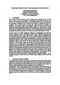
Fig. 1. Jobs in a system employing BSAC with a batch size of 5 jobs.
4. While the current time < Tnext a. For each job received: i. If it has a low priority, send the job to the low priority queue ii. If it has a high priority i. If the total size of jobs in the waiting batch + the job size < the batch size a. Admit the job into the waiting batch ii. Else a. Reject the job 5. Transfer the waiting batch to the current batch 6. Set the next batch start time, Tnext = current time + T 7. Repeat 4–6 Figure 1 gives an example of a BSAC system with a given batch size of 5 jobs. Starting from time t 0 , the jobs numbered 0–9 arrive dynamically. At times t 2 and t4 , the jobs in the waiting batch are moved to the current processing batch. At times t 1 and t3 , the batch is full. Since jobs 0–9 each arrive at a time when the waiting batch is not full, they are accepted. Any jobs arriving between times t 1 and t2 , or t3 and t4 , would be rejected. In a computer and network system that admits all arriving jobs, job waiting times depend on the jobs’ variable arrival times. As a result, the number of jobs waiting in the system (the system load) is unbounded. We expect the BSAC method to assist in reducing the variance in job waiting times because it bounds the size of each batch, and at any given time a bounded batch is processed for service. Each job’s waiting time consists of the waiting time in the waiting batch and the waiting time in the current batch, since each job in the current batch still needs to take its turn for service by the resource. The time in the waiting batch is bounded, based on the schedule imposed by T . The waiting times of the jobs in the current batch are different but are bounded due to the bounded batch size. Hence, the total waiting time of each job in a computer/network system with BSAC can become predictable by reducing the variance of waiting times. The BSAC method allows the introduction of static job scheduling methods to further reduce WTV. 2.3. Job scheduling methods All jobs in a computer/network system with no admission control, as well as jobs in the current batch of a system with BSAC, must be scheduled for service individually by a system resource. Job scheduling
N. Ye et al. / Batch scheduled admission control for computer and network systems
1
2
3
Job
Processing time
Level
Co-level
1
3
7
3
2
4
4
7
3
2
2
5
215
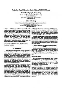
Fig. 2. Sample problem indicating precedence graph, level and co-level of jobs.
determines the order in which to process a set of jobs. Since the job scheduling method is not the focus of this study, we select a number of representative job scheduling methods available in existing literature to observe if the differences among job scheduling methods has an effect on the WTV of a computer/network system with no admission control versus one with BSAC. Casavant and Kuhl give a taxonomy of job scheduling methods for distributed computing systems [21]. There are also many scheduling methods developed for production planning in manufacturing [22]. Additionally, many other scheduling methods exist [23–25]. Among these job scheduling methods, we select five representative methods to be implemented in this study: First Come First Serve (FCFS), Shortest Processing Time (SPT), Weighted SPT (WSPT), Earliest Due Date (EDD), Highest Levels First with Estimated Times (HLFWET) and Smallest Co-Levels First with Estimated Times (SCFWET). The simplest job scheduling method we consider is FCFS, which is the most common job scheduling method on current computer and network systems [3]. FCFS schedules jobs for service in the same order that they arrive. The next three scheduling rules, SPT, WSPT and EDD, are common for production planning in manufacturing [22]. SPT schedules jobs in increasing order of their processing times, that is, the job with the shortest processing time is scheduled to be the first for service. WSPT considers the priority of jobs, along with their processing times, and schedules them in decreasing order of the ratio of priority to processing time. For instance, consider job 1 with processing time = 3, and priority = 4, and job 2 with processing time = 2 and priority = 3. The ratios for jobs 1 and 2 are 4/3 = 1.33 and 3/2 = 1.5 respectively. If both jobs are waiting for service, by the WSPT rule, job 2 is scheduled before job 1. EDD arranges jobs in the order of their respective due dates where the job with the earlier due date is scheduled to be the first for service. The next two scheduling methods we consider are known as list-scheduling algorithms [4], which are common in research work for computer and network systems. These two methods consider the precedence of jobs when scheduling them. For example, consider the three jobs in Fig. 2 with processing times indicated in the accompanying table. The graph shows the precedence relationship of the three jobs: job 1 must be completed before jobs 2 and 3. From the graph in Fig. 2, an entry vertex is one with no predecessors (job 1) and an exit vertex is one with no successors (jobs 2 and 3). The length of a path between an entry and exit vertex is the sum of the processing times of each vertex (job) on the path, including the entry and exit vertices (e.g. a path from 1 to 3 is of length 3 + 2 = 5). The level of a job is the longest path from its representative vertex to an exit vertex in the precedence graph. The co-level of a job is the longest path from an entry vertex to the job’s vertex. The table in Fig. 2 gives the levels and co-levels of the accompanying precedence graph. HLFWET schedules jobs in decreasing order of level. SCFWET schedules jobs in increasing order of co-level. By the HLFWET method, the jobs in Fig. 2 are processed in the order 1, 2, 3 and by the SCFWET method; 1, 3, 2.
216
N. Ye et al. / Batch scheduled admission control for computer and network systems
Fig. 3. Precedence graph of the 30 jobs in Problem 1.
3. Test examples This section presents two test examples to illustrate how BSAC can be used to improve the variance of job waiting times. Section 4 presents a simulation experiment to further test BSAC in comparison with no admission control. We develop two test problems, each consisting of a set of jobs requesting service. For each problem, we introduce two types of job arrival patterns: bursty and steady. In the bursty pattern, all jobs arrive simultaneously, while for the steady pattern, job arrival is spread out. There are two key differences between the two problems we describe in this section. First of all, the first problem has only 30 jobs, while the second has 3,000, for representing different problem sizes. Secondly, the jobs in the first problem come with associated information (job precedence, due date and priority) along with processing time, while the jobs in the second problem have only information of processing time, for representing jobs in different service environments. We describe these two problems, along with their job arrival patterns and the application of BSAC in this section. 3.1. Problem 1 Problem 1 has 30 jobs requesting service from a single resource, with a precedence graph as shown in Fig. 3. The vertices of the graph in Fig. 3 indicate the 30 jobs and are labeled with the respective job numbers, while the edges indicate the precedence relationship. These jobs have processing times with values ranging from 1 to 21, due dates ranging from 1 to 15, and priorities ranging from 1 to 11, which are all generated using a uniform distribution, and are shown in Table 1. The level and co-level columns in Table 1 are computed using the definitions of the HLFWET and SCFWET methods given in Section 2.3. Two job arrival patterns are considered. Under the bursty arrival condition, all jobs arrive at once. Under the steady arrival condition, a moderate number of jobs arrive at different intervals. We allow
N. Ye et al. / Batch scheduled admission control for computer and network systems
217
Table 1 Description of the 30 jobs in Problem 1 Job 1 2 3 4 5 6 7 8 9 10 11 12 13 14 15 16 17 18 19 20 21 22 23 24 25 26 27 28 29 30
Processing time (1 to 21) 8 4 5 10 2 10 20 16 9 13 5 12 2 10 19 3 10 15 17 17 21 19 8 13 16 17 6 7 20 16
Due date (1 to 15) 13 1 11 14 14 1 13 3 11 15 14 11 11 6 11 7 1 11 9 15 6 8 13 15 6 2 2 4 5 5
Priority Weight (1 to 11) 7 8 6 2 11 4 5 6 6 3 3 6 7 9 9 2 6 11 9 5 9 7 1 10 5 9 10 7 6 10
Level
Co-Level
91 71 53 79 83 56 67 48 69 81 46 47 32 60 68 41 35 30 50 49 38 25 15 33 32 17 6 7 20 16
8 12 13 18 10 18 32 29 27 23 23 44 31 37 42 26 54 46 54 59 47 73 54 67 75 64 79 61 87 91
the overlapping of the arrival times of groups of jobs in the steady arrival condition to see the effect of admission control. To simulate these conditions, we set the jobs to arrive in sets as represented by the dashed ovals in Fig. 3 and adjust the time-between-arrival (TBA) of the sets in the system. For the bursty condition, we use a TBA of 0 time unit so that all 30 jobs arrive and request service at the same instant. For the steady condition, we use a TBA of 25 time units. For example, the first set arrives at time 0, the second set at time 25, the third set at time 50, and so on. We use 25 here because we observe that the total processing time of each set is greater than 25, thus we ensure that jobs from the current set are still being processed for service when the next set arrives, giving us the desired overlapping condition to see the effect of admission control. For BSAC, jobs are processed in batches. We let batches comply with sets of jobs that are clearly separated by the precedence relationships. The dashed ovals in Fig. 3 show how the jobs in Problem 1 are batched. We set T to 100 time units because we observe that the total processing time of each batch in Figure 3 is less than 100. Hence, this value ensures that all jobs in the current batch can complete processing within the time interval of T . Since the next batch does not start processing until the end of the time interval for processing the current batch, applying BSAC to the bursty and steady patterns of jobs produces the same effect as the batches arriving by a TBA of 100 time units. Hence, we indicate the application of BSAC with TBA = 100.
218
N. Ye et al. / Batch scheduled admission control for computer and network systems
All of the five scheduling methods are implemented for Problem 1. In both systems, with and without admission control, the waiting time for each job is calculated based on the order in which jobs are scheduled for service. Each of the two systems under each arrival condition using each scheduling method produces a schedule of jobs. Given a schedule of the 30 jobs, the waiting time of a job is equal to the sum of the processing times of the jobs preceding it. Then we can calculate the mean and variance of the waiting times for all 30 jobs. For a given scheduling method, we can then compare the variance of job waiting times for both systems. 3.2. Problem 2 We consider a web server as the computer/network system, and create Problem 2 with 3,000 jobs (web requests) whose job sizes (sizes of requested web pages or files) follow a Pareto distribution since existing literature indicates this type of distribution for web servers [26,27]. We use the OPNET Modeler software to generate the 3,000 jobs according to a Pareto distribution with a shape parameter of 1.4 and scale parameter of 65,536. We choose the parameters empirically so that the mean job size is (1.4*65,536) / (1.4–1) = 229.376 bits, which is about 28 K bytes and represents a typical job size on a web server [26,27]. The service rate of our simulated computer/network system is 12,697,600 bits per second and the processing time of a job is its size divided by the service rate. Therefore, we know that on average the server can serve about 12,697,600 / 229,376 = 55 jobs per second. As in Problem 1, we consider two job arrival patterns: bursty and steady. In the bursty condition, the inter-arrival times of the jobs are constant with a value of 3.3*E-08 and the jobs are generated from time = 100 to time = 100.0001. For the steady condition, we constrain the jobs to arrive in 5 sets of 600 jobs each arriving at times 100, 106, 112, 118, and 132 respectively since we know that 600 jobs take about 600/55 = 11 seconds to process, thus the arrival pattern used produces the desired overlapping of job sets. To apply BSAC, we let the batches comply with the five job sets. We set the time slot of processing each batch to be T = 30 seconds to ensure that the server completes processing each batch within time T . Since the next batch does not start processing until the end of the time slot for processing the current batch, applying BSAC to the bursty and steady patterns of jobs produces the same effect as when the batches arrive by TBA of 30 seconds. Hence, we indicate the application of BSAC with TBA = 30. That is, it is as if the five batches arrive at times 100, 130, 160, 190, and 220. For problem 2, we have 3000 jobs with no priority, due date or precedence. From the definitions of the scheduling methods, we see that four of the six scheduling methods require at least one of these parameters to be present: WSPT, EDD, HLFWET and SCFWET. As a result, we can only consider two scheduling methods: FCFS and SPT. Hence, only FCFS and SPT are implemented for Problem 2. Each of the two systems with BSAC and with no admission control under each arrival condition using each scheduling method produces a schedule of jobs. For a given schedule of jobs, we compute the waiting time of each job, along with the mean and variance of job waiting times for all the jobs, in the same manner as for Problem 1. The variance performance data are then used to compare BSAC and no admission control. 3.3. Results and discussions Figure 4 shows the variance of job waiting times under each arrival condition using each system and each scheduling method for Problem 1. In each of the plots in Fig. 4, the y-axis is the job waiting time and the x-axis is the job number. There are three lines in each plot: TBA = 0 (blue or dark line) repre
N. Ye et al. / Batch scheduled admission control for computer and network systems
a)
b)
c)
d)
e)
f)
219
Fig. 4. Job waiting times under a) FCFS, b) SPT, c) WSPT, d) EDD, e) HLFWET and f) SCFWET in Problem 1.
sents a system with no admission control and bursty condition, TBA = 25 (purple or medium-dark line) represents a system with no admission control and steady condition, and TBA = 100 (yellow or light line) represents a system with BSAC under either arrival condition. In Fig. 4, the yellow or light lines indicating the waiting times of the jobs when BSAC is used (corresponding to TBA = 100) are significantly smoother in each plot than when there is no admission control (in the cases of TBA = 0 and TBA = 25). Smoother lines mean that the variability in the job waiting times is much smaller when BSAC is used. Tables 2 and 3 give the mean and variance values of the job waiting times. Table 2 shows the mean job waiting times under all scheduling methods for each of the systems and arrival conditions, while Table 3 shows the variance of the job waiting times. These tables indicate an improved performance for both mean and variance when BSAC is employed,
220
N. Ye et al. / Batch scheduled admission control for computer and network systems Table 2 Mean of job waiting times for all experiments in Problem 1 Scheduling method FCFS SPT WSPT EDD HLFWET SCFWET
No admission control and bursty pattern 148.8 119 137 171 161.1 142.27
No admission control and steady pattern 89.06 40 51 72.67 65.63 54.07
Admission control with BSAC 21.16 16 18.3 21.37 25.3 17.97
Table 3 Variance of job waiting times for all experiments in Problem 1 Scheduling method FCFS SPT WSPT EDD HLFWET SCFWET
No admission control and bursty pattern 148.8 10257 11973.67 10944.73 11291.42 10941.06
No admission control and steady pattern 89.06 3080.62 4095.51 5092.29 4619.90 3806.60
Admission control with BSAC 21.16 282 355.28 361.23 450.54 323.30
Table 4 Mean of job waiting times for all experiments in Problem 2 Scheduling method FCFS SPT
No admission control and bursty pattern 23.7888 12.072
No admission control and steady pattern 10.1991 3.0395
Admission control with BSAC 5.3662 2.4139
Table 5 Variance of job waiting times for all experiments in Problem 2 Scheduling method FCFS SPT
No admission control and bursty pattern 240.5122 93.0607
No admission control and steady pattern 30.9732 19.193
Admission control with BSAC 11.9975 3.752
compared to a system with no admission control, regardless of which scheduling method is used and which job arrival condition is considered. Tables 4 and 5 indicate that for Problem 2 the mean and variance of the job waiting times with BSAC are smaller than those with no admission control, regardless of which scheduling method is used and which job arrival condition is considered. Hence, BSAC aids in improving the mean and variance of job waiting times for these job sets. 4. Experiments In this section, we design a simulation experiment to test a system with BSAC against a system using no admission control; for both systems, we employ the FCFS scheduling method. The goal is to show the performance effect of BSAC alone on job WTV under various conditions, and evaluate its sacrifice on mean waiting time.
N. Ye et al. / Batch scheduled admission control for computer and network systems
221
WTM 2500 2000 1500
FCFS BSAC
1000 500 0 1 2 3 4 5 6 7 8 9 1011 1213 141516 171819 2021 222324
Fig. 5. Waiting Time Mean for the experiments in Table 6.
4.1. Setup In this system we have a source node, a router node, and a sink node. Pre-pended to the router is the BSAC method. Thus, jobs traverse the system logically from source, to BSAC, to router, to sink. We experiment with four factors: job size, job inter-arrival time, batch size, batch start time interval. Levels on the factors are chosen to cover a variety of traffic and BSAC configuration conditions. The source node generates traffic. We create 100 jobs, with a normal size distribution using a mean of 100 bytes. We experiment with two levels of job size standard deviation: 25 and 40 bytes. The jobs are sent out with two levels of job inter-arrival time using an exponential distribution with a mean of 100 and 80 ms. These inter-arrival times simulate normal and heavy traffic loads, respectively. The sink node is simply there to collect the jobs sent by the router. The router in our system runs at 1 byte/ms which is the service rate of data transmission. This sets our router speed to match the normal traffic load. For BSAC, we noted previously that there are a number of ways to set the batch size. For this experiment, we choose to consider a batch size based on the number of jobs each batch can hold. The two levels of batch size we choose are 10 and 20. We also experiment with varying levels of batch start interval times. First, we compute T = (batch size*avg job size)/router speed
to get the expected time to process a batch. Then we set three levels equal to 90, 100, and 110 percent of T . Thus we have 2 (job size standard deviations) × 2 (job inter-arrival times) × 2 (batch sizes) × 3 (batch start interval times) = 24 experiment scenarios. For each scenario, we run the system with FCFS alone, and with BSAC + FCFS, for a total of 48 simulation runs. 4.2. Results and discussions We collect actual system time at the point each job arrives at the router, or is admitted into the waiting batch for BSAC, and the point that it begins processing on the router. Then we take the difference between these times. Thus, the results in this section consider total waiting time in the router, including the waiting time in the waiting batch and the waiting time in the current batch. To evaluate performance and tradeoffs, we compute both the waiting time mean (WTM) and WTV for the set of 100 jobs under
222
N. Ye et al. / Batch scheduled admission control for computer and network systems Table 6 Waiting Time Mean for the experiments outlined in Section 4 Scenario 1 2 3 4 5 6 7 8 9 10 11 12 13 14 15 16 17 18 19 20 21 22 23 24
Job Size STD 25 25 25 25 25 25 25 25 25 25 25 25 40 40 40 40 40 40 40 40 40 40 40 40
Interarrival 100 100 100 100 100 100 80 80 80 80 80 80 100 100 100 100 100 100 80 80 80 80 80 80
WTM Batch Size 10 10 10 20 20 20 10 10 10 20 20 20 10 10 10 20 20 20 10 10 10 20 20 20
%Time
FCFS
BSAC
90 100 110 90 100 110 90 100 110 90 100 110 90 100 110 90 100 110 90 100 110 90 100 110
412 405 405 372 400 405 1108 1103 1108 1104 1104 1100 434 433 433 433 433 433 1096 1098 1090 1096 1097 1101
936 935 1065 1768 1968 2094 990 1085 1147 2048 2160 2340 973 965 1074 1786 1996 2115 1007 1161 1206 1191 1189 1334
WTV 700000 600000 500000 400000
FCFS
300000
BSAC
200000 100000 0 1 2 3 4 5 6 7 8 9 101112131415161718192021222324
Fig. 6. Waiting Time Variance for the experiments in Table 7.
each of the 24 scenarios. Tables 6 and 7 show WTM and WTV results respectively. Each row in the table represents a simulation scenario. Figures 5 and 6 present bar graphs of the data in Tables 6 and 7. We first observe that the difference in two job size standard deviations (the difference between scenarios 1–12 and scenarios 13–24) has little effect on the pattern of the plots in Figs 5 and 6. We also note that the effect of three different batch start time intervals (90, 100 and 110), is noticeable, but is overshadowed
N. Ye et al. / Batch scheduled admission control for computer and network systems
223
Table 7 Waiting Time Variance for the experiments outlined in Section 4 Scenario 1 2 3 4 5 6 7 8 9 10 11 12 13 14 15 16 17 18 19 20 21 22 23 24
Job Size STD 25 25 25 25 25 25 25 25 25 25 25 25 40 40 40 40 40 40 40 40 40 40 40 40
Interarrival 100 100 100 100 100 100 80 80 80 80 80 80 100 100 100 100 100 100 80 80 80 80 80 80
Batch Size 10 10 10 20 20 20 10 10 10 20 20 20 10 10 10 20 20 20 10 10 10 20 20 20
WTV %Time 90 100 110 90 100 110 90 100 110 90 100 110 90 100 110 90 100 110 90 100 110 90 100 110
FCFS
BSAC
80919.81202 79819.08646 78325.73737 68638.41 76542.0303 78268.41657 563235.4435 551804.9506 557023.7668 553054.7146 554811.3838 544119.8954 107632.1991 106281.0565 106492.3754 106329.7782 107774.7721 106376.6057 603984.3026 609403.537 599929.7829 605088.3838 607282.9151 614995.8031
36820.05353 35389.11897 24995.73643 97154.18146 70005.94904 72799.67067 29069.38811 38256.03258 22057.53943 118718.6466 89490.09351 75242.01519 45369.61954 44520.68591 42653.99469 106581.1804 69540.93151 80635.36136 44297.84898 54639.92842 35583.19337 126640.1405 143295.0179 60200.62278
by the effects of inter-arrival time and batch size. Thus, we focus our discussions on these two factors. Under a normal traffic scenario (inter-arrival time of 100 ms in scenarios 1–6 and 13–18), FCFS shows a much better WTM. If we consider the WTV under normal traffic, we see that BSAC shows improvement over FCFS in all cases where we use a batch size of 10 (in scenarios 1–3 and 13–15). For a batch size of 20, BSAC and FCFS have similar WTV, with BSAC being marginally better in overall. Thus, we conclude that under the normal traffic condition, with a batch size of 10, BSAC provides better WTV with a sacrifice in mean approximately double to that of FCFS. In the heavy traffic scenario (inter-arrival time of 80ms in scenarios 7–12 and 19–24), BSAC shows a similar WTM to FCFS when the batch size is 10, and about twice as much when its 20. For WTV, we see that BSAC is considerably better than FCFS for both batch sizes, and more so for a batch size of 10. Thus, we conclude that under the heavy traffic condition and a batch size of 10, BSAC provides much better WTV with little or no sacrifice in mean. 5. Conclusion Minimizing the variance in the waiting times of jobs in a computer/network system is a key factor in assuring the timeliness aspect of QoS. Job scheduling and admission control are two areas to consider when working towards this goal. In this paper, we focus on admission control. We introduce a batch scheduled admission control method to admit jobs in batches of a given size which are processed for service in such a way that one batch of jobs has completed processing before another batch begins. The BSAC method can be applied to high priority jobs in a system and changes the dynamic queuing problem
224
N. Ye et al. / Batch scheduled admission control for computer and network systems
into a static problem which allows the introduction of job scheduling techniques that can further reduce job waiting time variance but require a static set of jobs to operate on. This method is also useful in other domains, such as manufacturing and resource scheduling. We provide examples of how this method can be employed. The results of our method in comparison with no admission control on two test problems illustrate how the BSAC method can assist in providing a smaller variance and thus better predictability of job waiting times when compared to a system with no admission control. These results hold for both bursty and steady job arrival conditions, regardless of the scheduling method, problem sizes, or distribution of processing times. In these two test problems, only job waiting time in the current batch is considered. However, in the simulation experiments described in Section 4, the sum of job waiting time in the waiting batch and job waiting time in the current batch are considered. These simulation experiments showing conditions in which BSAC lowers WTV. Specifically, we show that BSAC can provide considerably better performance in minimizing WTV with little or no sacrifice in the mean waiting time under certain conditions. Hence, we show how BSAC can be used alone, or in combination with various job scheduling methods to improve the invariance of job waiting times. BSAC allows for the application of any scheduling methods that require a static set of jobs. Due to the operation of BSAC, the processing system sees jobs as arriving in batches rather than dynamically, and can thus consider each batch as a static set of jobs. Hence, in our example application of BSAC, we are able to introduce a job scheduling method, which has shown to increase the stability of job waiting times for a batch of jobs [28]. The combined use of BSAC and our novel scheduling method can provide a significant performance increase with regard to job waiting time invariability when compared to systems without admission control and/or those which use other job scheduling methods. Note that BSAC is also applicable to systems in other fields that also require service predictability. The concept of BSAC is different than that of dynamic queuing schemes (such as M/M/1 and G/G/1/K) seen in literature. BSAC aims to change the common dynamic queuing problem into a static one, allowing for the introduction of job scheduling techniques that require a static set of jobs to operate on. In order to implement BSAC in a computer or network system, we suggest the following considerations. It is necessary to provide mechanisms for separating jobs into buffers to differentiate processing and waiting batches. An admission control mechanism also needs to be in place to determine when a job will be admitted into the waiting batch. Additional mechanisms are required for moving jobs from the waiting batch to the processing batch triggered by time slots and announcing to service requesting systems when the next batch will begin processing. In our examples and simulation experiments, we assume that low priority jobs do not effect the processing of high priority jobs, and are processed on this resource only when it is idle. This assumption requires further investigation to determine how low priority jobs are handled, for example, does a high priority job pre-empt one of lower priority? We envision that BSAC would be useful in a complete system design that we are currently investigating. This design includes mechanisms that determine when a high priority batch is processed, and ensures that high priority jobs are not rejected in absence of a communication fault. In this study, we consider only the waiting times of admitted jobs, and do not make accommodations for rejected or low priority jobs. This study addresses primarily job waiting time. Dropped and delayed jobs are not investigated are not investigated in this study, but will be addressed in our future research.
N. Ye et al. / Batch scheduled admission control for computer and network systems
225
Acknowledgements This work is sponsored by the Air Force Research Laboratory – Rome (AFRL-Rome) under grant number F30602-01-1-0510, and the Department of Defense (DoD) and the Air Force Office of Scientific Research (AFOSR) under grant number F49620-01-1-0317. The US government is authorized to reproduce and distribute reprints for governmental purposes notwithstanding any copyright annotation thereon. The views and conclusions contained herein are those of the authors and should not be interpreted as necessarily representing the official policies or endorsements, either express or implied, of, AFRL-Rome, DoD, AFOSR, or the US Government. We thank anonymous reviewers for their helpful comments. References [1] [2] [3] [4] [5] [6] [7] [8] [9] [10] [11] [12] [13] [14] [15] [16] [17] [18] [19] [20] [21] [22]
Y. Chen, T. Farley and N. Ye, QoS requirements of network applications on the Internet, Information, Knowledge, Systems Management 4(1) (2003), 55–76. N. Ye, QoS-centric stateful resource management in information systems, Information Systems Frontiers 4(2) (2002), 149–160. J. Kurose, Open issues and challenges in providing Quality-of-Service guarantees in high-speed networks, ACM SIGCOMM Computer Communication Review 23(1) (1993), 6–15. A.G. Merten and M.E. Muller, Variance minimization in single machine sequencing problems, Management Science 18(9) (1972), 518–528. S. Eilon and I.G. Chowdhury, Minimizing Waiting Time Variance in the Single Machine Problem,’ Management Science 23(6) (1977), 567–574. L. Schrage, Minimizing the time-in-system variance for a finite jobset, Management Science 21(5) (1975), 540–543. J. Mittenthal, M. Raghavachari and A.I. Rana, V- and Λ-shaped properties for optimal single machine schedules for a class of non-separable penalty functions, European Journal of Operational Research 86(2) (1995), 262–269. U. Al-Turki, C. Fediki and A. Andijani, Tabu search for a class of single-machine scheduling problems, Computers & Operation Research 28(12) (2001), 1223–1230. G. Viswanathkumar and G. Srinivasan, A branch and bound algorithm to minimize completion time variance on a single processor, Computers & Operations Research 30(8) (2003), 1135–1150. P. De, J.B. Ghosh and C.E. Wells, Scheduling to minimize the coefficient of variation, Int’l Journal of Production Economics 44(3) (1996), 249–253. W. Kubiak, J. Cheng and M.Y. Kovalyov, Fast fully polynomial approximation schemes for minimizing completion time variance, European Journal of Operational Research 137(2) (2002), 303–309. W. Kubiak, New results on the completion time variance minimization, Discrete Applied Mathematics 58(2) (1995), 157–168. X. Cai, V-shape property for job sequences that minimize the expected completion time variance, European Journal of Operational Research 91(1) (1996), 118–123. D.K. Manna and V.R. Prasad, Pseudopolynomial algorithms for CTV minimization in single machine scheduling, Computers & Operations Research 24(12) (1997), 1119–1128. X. Lu, R.A. Sitters and L. Stougie, A class of on-line scheduling algorithms to minimize total completion time, Operations Research Letters 31(3) (2003), 232–236. J.J. Kanet, Minimizing variation of flow time in single machine systems, Management Science 27(12) (1981), 1453–1459. N.G. Hall and W. Kubiak, Proof of a conjecture of Schrage about the completion time variance problem, Operations Research Letters 10(8) (1991), 467–472. V. Vani and M. Raghavachari, Deterministic and random single machine sequencing with variance minimization, Operations Research 35(1) (1987), 111–120. W. Kubiak, Completion time variance minimization on a single machine is difficult, Operations Research Letters 14(1) (1993), 49–59. D.K. Manna and V.R. Prasad, Bounds for the position of the smallest job in completion time variance minimization, European Journal of Operational Research 114(2) (1999), 411–419. T.L. Casavant and J.G. Kuhl, A taxonomy of scheduling in general-purpose distributed computing systems, IEEE Transactions on Software Engineering 14(2) (1988), 141–154. M. Pinedo, Scheduling Theory, Algorithms, and Systems, Englewood Cliffs, NJ: Prentice-Hall, Inc., 1995.
226 [23] [24] [25] [26] [27] [28]
N. Ye et al. / Batch scheduled admission control for computer and network systems T.L. Adam, K.M. Chandy and J.R. Dickson, A comparison of list schedules for parallel processing systems, Communications of the ACM 17(12) (1974), 685–690. L. Epstein, J. Noga and G.J. Woeginger, On-line scheduling of unit time jobs with rejection: minimizing the total completion time, Operations Research Letters 30(6) (2002), 415–420. P. De, J.B. Ghoshbs and C.E. Wells, Scheduling to minimize the coefficient of variation, International Journal of Production Economics 44(3) (1996), 249–253. J. Gordon, Pareto process as a model of self-similar packet traffic, Global Telecommunications Conference 1995 (GLOBECOM ’95), IEEE 3 (1995), 2232–2236. M.F. Arlitt and C.L. Williamson, Web server workload characterization: the search for invariants, ACM SIGMET-RICS’96 (May 1996), 126–137, Extended version. N. Ye, X. Li and T. Farley, Job scheduling method for reducing waiting time variance, Computers & Operations Research in press (available online).
Nong Ye is a Professor of Industrial Engineering at Arizona State University (ASU). She holds a Ph.D. degree in Industrial Engineering from Purdue University, West Lafayette, Indiana, and a M.S. degree and a B.S. degree in Computer Science from the Chinese Academy of Sciences and Peking University, China, respectively. She is the Director of the Information and Systems Assurance Laboratory at ASU. Her research work focuses on security, dependability and Quality of Service (QoS) of computer and network systems. She is an Editor for IEEE Transactions on Systems, Man, and Cybernetics and an Associate Editor for IEEE Transactions on Reliability and Information, Knowledge, Systems Management.
Toni Farley is a doctoral student of Computer Science at Arizona State University (ASU), Tempe, Arizona. She is studying under a Graduate Fellowship from AT&T Labs – Research. Her research interests include networks, security, graph theory and combinatorics. She holds a B.S degree in Computer Science and Engineering from ASU. She is a member of IEEE and the IEEE Computer Society.
Xueping Li is an Assistant Professor of Industrial and Information Engineering and Director of the Intelligent Information Engineering Systems Laboratory at the University of Tennessee – Knoxville. He holds a Ph.D. from Arizona State University.
Harish Bashettihalli currently works with Oracle Corporation as a Member of Technical Staff and works on application software development. He holds a Master of Science degree in Computer Science from Arizona State University and a Bachelors degree in Computer Science from Bangalore University. His research focus at Arizona State University was on computer and network intrusions.