BAYESIAN AFFINE TRANSFORMATION OF HMM PARAMETERS FOR INSTANTANEOUS AND SUPERVISED ADAPTATION IN TELEPHONE SPEECH RECOGNITION Jen-Tzung Chien a, Hsiao-Chuan Wang a and Chin-Hui Lee b a Department of Electrical Engineering, National Tsing Hua University, Hsinchu, Taiwan b Multimedia Communications Research Lab, Bell Laboratories, Murray Hill, USA
[email protected] [email protected] [email protected]
ABSTRACT This paper proposes a Bayesian affine transformation of hidden Markov model (HMM) parameters for reducing the acoustic mismatch problem in telephone speech recognition. Our purpose is to transform the existing HMM parameters into its new version of specific telephone environment using affine function so as to improve the recognition rate. The maximum a posteriori (MAP) estimation which merges the prior statistics into transformation is applied for estimating the transformation parameters. Experiments demonstrate that the proposed Bayesian affine transformation is effective for instantaneous adaptation and supervised adaptation in telephone speech recognition. Model transformation using MAP estimation performs better than that using maximum-likelihood (ML) estimation.
works, the affine transformation parameters were estimated via the ML theory which no prior information was considered. However, if a proper prior knowledge is available to model transformation, we can use the maximum a posteriori (MAP) principle [7] to estimate the transformation parameters. Using the transformed HMM parameters, the recognition performance may be further improved. In this study, we optimally estimate the affine transformation parameters η = ( A , b) by maximizing the posterior density which consists of a likelihood function and a prior density [8]. The expectation-maximization (EM) algorithm [9] is applied for the parameter estimation. In the experiments of telephone speech recognition, we evaluate the proposed method by using instantaneous adaptation, supervised adaptation and two-pass adaptation. The performance of ML and MAP affine transformation is compared and discussed. We also illustrate the asymptotic property of proposed method.
1. INTRODUCTION
2. BAYESIAN AFFINE TRANSFORMATION
To attain the automation of telephone services, it is necessary to develop the robust speech recognition algorithms [1-3] over telephone networks. A major problem of telephone speech recognition comes from the acoustic mismatch between training and testing environments. The mismatch sources due to speaker, ambient noise, telephone handset, transmission line, etc. may cause the serious degradation of recognition performance. However, many approaches are applicable to telephone speech recognition. One practical approach is to transform (or adapt) a given set of speech hidden Markov models (HMMs) using some transformation functions so that the transformed HMM parameters are close to a new telephone environment. Accordingly, the speaker adaptation techniques which adapt the speaker-independent (SI) HMM parameters to a new speaker are feasible to telephone speech recognition. In the literature, the model transformation using affine function y = Ax + b, such as the maximum likelihood linear regression (MLLR) [4] and the constrained transformation [5], has been successfully applied for speaker adaptation. Here, x and y represent the original sampled data and its transformed version, respectively. A and b are the parameters for affine transformation. Also, the maximum likelihood (ML) based stochastic matching method [6] employed the affine function for transforming the testing features to match with the given HMM parameters. In these
Model transformation using bias function y = x + b is a simple method for compensating the linear channel mismatch in adverse environment. In [10-11], the bias transformation parameter b was estimated via MAP theory and reduced the mismatch effect in telephone speech recognition. However, the bias transformation may be insufficient for compensating the variabilities in telephone environments. Consequently, we are motivated to introduce the affine function y = Ax + b for providing a more elaborate transformation than the bias function. Let Y = {y t } , S = {st } and L = {lt } denote the observation sequence, state sequence and mixture component sequence, respectively. Using affine transformation, the likelihood function of state n and mixture m generating y t is expressed by P( yt st = n, lt = m, η = ( A, b)) = ( 2π ) − D 2 AΣ n ,mA T
−1 2
⋅
1 exp− ( yt − Aµ n ,m − b) T ( AΣ n, mA T ) −1 ( yt − Aµ n ,m − b) . (1) 2 where {µ n,m , Σ n,m} are the Gaussian parameters of a HMM. A and b are random variables. In this study, we would like to apply the MAP framework to estimate the affine transformation parameters. Based on the
MAP theory, parameter estimation is performed by maximizing the posterior likelihood P(η Y) , or equivalently the product of a likelihood function P( Y η) and a prior density P(η) , as follows η MAP = arg max P(η Y) = arg max P( Y η) P(η) . η
η
(2)
Due to the incomplete data problem, Eq. (2) is usually solved via the EM algorithm [9]. According to EM algorithm, the MAP estimate η MAP is obtained by iteratively increasing the posterior likelihood P(η Y) of current estimate η
(3)
where {Y,S,L} is the set of complete data. To adjust the contribution of the likelihood function and the prior density in MAP estimation, we introduce a tuning factor α [11] into Eq. (3). This tuning factor can serve as a compensating factor for adjusting the importance of the contributions from these two terms. Since the exact posterior density is usually unknown and uneasy to specify, this tuning factor may provide a method to tune the performance according to the amount of adaptation data and the goodness of the existing HMM parameters. The new estimate η ′ is then obtained by applying the following
η′ = {a ′, b′} = arg min F (a ′, b′) , where F (a ′ ,b ′ )
( y − a ′µ n,m − b′) 2 α ∑ ∑ ∑ γ t (n, m) t + log a ′ 2σ 2n ,m 2 2 a ′ σ n ,m , (7) = t n m 2 2 − 1 α ( ) σ (a ′ − µ a ) − 2rσ aσ b (a ′ − µ a ) + ⋅ b σ 2σ 2 (1 − r 2 ) (b′ − µ b ) + σ 2a (b ′ − µ b ) 2 a b
and
γ t ( n, m) = P( st = n, lt = m Y,a, b)
posterior
( yt − a ′µ n ,m ) α ∑ ∑ ∑ γ t (n, m) σ 2n ,m t n m 2 (1 − α )a ′ r (a ′ − µ a ) + µb 1− r2 σ σ σ b2 a b n m
+ .
γ t (n, m) (1 − α ) a ′2 + 2 σ 2n, m σ b (1 − r 2 )
(8)
(4)
then
M-step, we confirm that the posterior likelihood will never decrease. In Eq. (4), when α = 0.5, the conventional MAP estimation is produced. When α = 1, The MAP estimation becomes ML estimation. Besides, we assume that the scaling matrix A and the HMM covariance matrix Σ n,m of state n and mixture m are diagonal, i.e. A = diag( a ) and Σ n ,m = diag(σ 2n ,m ) . Then, the
L D} can be
independently derived for each vector component. For simplicity, we drop the dimension index i in the following expression. To derive the formula for a given density function, we further assume that the parameters a and b are Gaussian distributed, i.e. a ~ N ( µ a ,σ 2a ) and b ~ N ( µb , σ b2 ) . Because of the dependent property of parameters a and b [8], the joint prior density P (a , b) is modeled by a joint Gaussian density of this form
the
zero, we can derive the optimal parameter b′ as follows
Unfortunately, there is no close-form solution for the optimal parameter a ′ . Thus, we apply the steepest-descent algorithm [12] for iteratively searching the optimal parameter, i.e.
P(η′ Y) ≥ P(η Y) . Thus, by iteratively performing E-step and
affine transformation parameters η = {ai , bi , i = 1,
is
probability of staying in state n and mixture m given that the current parameters η = ( a , b) generate Y. In Eqs. (6-7), differentiating F ( a ′ , b′ ) with respect to b′ and setting it to
t
Q(η′ η) ≥ Q(η η)
(6)
{a ′ ,b ′}
α∑∑∑
η′
It can be proved [9] that if
(5)
where r is the correlation coefficient of parameters a and b. Under these assumptions for each dimension, Eq. (4) can be replaced by
b′ = η′ = arg max Q(η′ η) = η′
⋅
2πσ aσ b 1 − r 2
(a − µ a ) 2 (a − µ a )(b − µ b ) (b − µ b ) 2 1 exp − r 2 − + 2 2 σ aσ b σ b2 2(1 − r ) σ a
weighted version of maximization step (M-step)
arg max E {α log P( Y, S , L η′ ) + (1 − α ) log P(η′) Y, η} .
1
and
deriving the new estimate η ′ in an optimal sense. The first step (E-step) of EM algorithm is to calculate the expectation (or auxiliary) function given by Q(η′ η) = E {log P( Y, S , L η′) + log P(η′) Y,η} ,
P(η) = P(a ,b) =
a ′( l +1) = a ′ ( l ) − ρ
dF ( a ′, b′) da ′
a ′= a ′ ( l ) ,b ′= b′ ( l )
,
(9)
where ρ is a positive-valued step size and l is the iteration index. Using Eqs. (6-9), the new affine transformation parameters η ′ = ( a ′ , b ′) can be jointly and iteratively calculated with this generalized EM (GEM) algorithm. In general, this set of formulas is also referred to as the forwardbackward MAP estimate [7] which is analogy with the BaumWelch algorithm [13] for ML estimation.
3. SEGMENTAL MAP ESTIMATE Actually, the Bayesian affine transformation can be also implemented via the segmental MAP estimate [7-8]. Using this approach, the joint posterior likelihood of parameter η and state sequence S, P(η, S Y) , is maximized. The estimate procedure becomes
η
S
arg max max P( Y, S η) P(η) . η
(10)
S
Starting with any estimate η ( l ) and alternately maximizing P(η, S Y) over S and η, we guarantee that the values of P(η, S Y) are non-decreasing. Further, Eq. (10) can be divided into the following two equations S( l ) = arg max P(Y, S η(l ) ) ,
(11)
S
η( l +1) = arg max P( Y, S( l ) η) P(η) .
(12)
η
That is, the most likely state sequence S ( l ) is first decoded by the Viterbi algorithm [14]. Given the most likely state sequence S ( l ) , the new MAP estimate η ( l +1) is then obtained by using Eq. (12). Once again, we can apply the EM algorithm for solving Eq. (12). Using EM algorithm, it can be shown that the reestimation Eqs. (6-9) still hold for this segmental MAP estimation with γ t (n, m) = δ ( st( l ) − n)
∑
ω n ,m N ( yt ; µ n,m ,σ n2 ,m , η) K ω N ( yt ; µ n ,m ,σ n2,m ,η) k =1 n , k
,
(13)
where ω n ,m is the mixture gain, K is the mixture number of a HMM state and δ is the Kronecker delta function.
4. EXPERIMENTS A multispeaker (37 males and 36 females) recognition task for 250 Chinese names [8] was conducted to demonstrate the merits of proposed method. Our speech corpora were provided by Telecommunication Laboratories, Chunghwa Telecom Co., Ltd., Taiwan, R.O.C. The speech signal was sampled at 8kHz. The feature vector was characterized by 12 LPC-derived cepstral coefficients, 12 delta cepstral coefficient, 1 delta log energy and 1 delta delta log energy. In testing session, a total of 1000 testing utterances were collected through the telephone networks. Ten telephone handsets were used. In training session, a speech corpus consisted of 5045 phonetically-balanced Mandarin words (spoken by 51 males and 50 females) was prepared. This corpus was recorded in an office room via a high-quality microphone. We use this corpus to train the HMM parameters covering the acoustics of 408 Mandarin syllables. The tonal information of Mandarin was not considered here. Each Mandarin syllable is composed of an initial (or consonant) and a final (or vowel). Within a Mandarin syllable, the initial has strong coarticulation with the final. Hence, we employed the context-dependent subsyllable modeling scheme in our training procedure. Each HMM state parameter was modeled by a mixture Gaussian density with four mixture components. In proposed method, a shared transformation function is computed for adapting all HMM
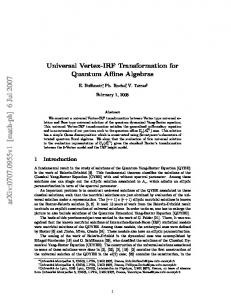
state parameters. The Bayesian affine transformation is implemented via the segmental MAP estimation. The speech recognizer without model transformation is referred to the baseline system. In MAP estimation, the hyperparameters of the prior 2 2 density, Θ = ( µ a , σ a , µ b , σ b , r ) , are crucial for parameter estimation. To adequately reflect the variabilities of model transformation, we sampled 80 telephone utterances from a different corpus. Each sampled utterance was uttered by a different speaker which was excluded from those speakers in testing database. For each utterance, we calculate the corresponding ML estimate of affine transformation parameter η ML by substituting α = 1 in Eqs. (6-9). Then, the hyperparameters Θ are determined by taking the operations of mean, variance and correlation coefficient over these 80 sets of ML estimates [8]. To assess the performance of proposed method, we perform three adaptation techniques which are instantaneous adaptation, supervised adaptation and two-pass adaptation. The instantaneous adaptation is a run-time unsupervised adaptation which is performed on the unknown testing utterance. The supervised adaptation executes the adaptation using some known utterances which are uttered by the testing speaker. In our experiment, only one adaptation utterance for each testing speaker. There are totally 73 adaptation utterances included. Each adaptation utterance contained a Chinese name. In addition, the two-pass adaptation combines these two techniques by first performing supervised adaptation for each testing speaker and then further performing instantaneous adaptation for the transformed HMM parameters according to the unknown testing utterance. To illustrate the convergence speed of proposed method, we plot the average log likelihood score per frame versus the EM iteration number of Bayesian affine transformation using supervised adaptation in Fig. 1. We can see that the proposed method converges rapidly within two iterations. Its asymptotic property is accordingly established.
26 25 24
log-likelihood/frame
η MAP = arg max max P(η, S Y) =
23 22 21 20 19 18 17 16
0
2
4
6
8
10
12
14
iteration num ber
Figure 1: Convergence of Bayesian affine transformation.
The recognition rates of the baseline system and cepstral mean normalization (CMN) [15-16] are 37.3% and 79.4%, respectively. For comparison, the results of ML affine transformation are also included. In Table 1, we compare the recognition rates of three adaptation techniques for ML and MAP affine transformation under tuning factors of 0.7, 0.5 and 0.2. We can see that the proposed MAP affine transformation performs consistently better than the ML affine transformation for three adaptation techniques. The supervised adaptation outperforms the instantaneous adaptation for different tuning factors. It is because that the estimation accuracy of transformation parameters is assured when the true transcription of adaptation utterance is provided. Furthermore, we also find that the recognition rates of two-pass adaptation are higher than those of instantaneous adaptation and supervised adaptation. It reflects the merit of two-pass adaptation. Also, the results of α = 0.2 has better performance than those of α = 0.5 and α = 0.7. This implies the importance of prior information in MAP estimation. All these results are significantly superior to the CMN method with a word accuracy of 79.4%. From these results, we conclude that the proposed Bayesian affine transformation has good convergence property and recognition performance in telephone speech recognition.
Table 1 Recognition rates (%) of three adaptation techniques using ML and MAP affine transformation under various tuning factors instantaneous supervised two-pass adaptation adaptation adaptation ML 81.8 85.2 85.9 MAP (α=0.7) 82.4 86.1 86.7 MAP (α=0.5) 82.6 86.1 86.8 MAP (α=0.2) 82.9 86.5 87.1
5. CONCLUSION We propose the transformation-based adaptation based on the MAP framework and effectively apply it for telephone speech recognition. The estimation procedures using forwardbackward MAP and segmental MAP are derived. From the experimental results, we have the following conclusions; (1) The proposed approach converges rapidly. (2) The performance of MAP affine transformation is better than that of ML affine transformation. (3) The proposed approach can be employed in instantaneous adaptation, supervised adaptation and two-pass adaptation. (4) The proposed method is superior to CMN method.
6. ACKNOWLEDGMENT This research has been partially supported by the Telecommunication Laboratory, Chunghwa Telecom Co., Ltd., Taiwan, R.O.C., under contract TL-85-5203.
7. REFERENCES [1] C. H. Lee, On feature and model compensation approach to robust speech recognition , in Proc. ESCA-NATO Workshop on Robust Speech Recognition for Unknown Communication Channels, 1997. [2] Y. Gong, Speech recognition in noisy environments : A survey , Speech Communication, vol. 16, pp. 261-291, 1995. [3] B. H. Juang, Speech recognition in adverse environments , Computer Speech and Language, vol. 5, pp. 275-294, 1991. [4] C. J. Leggetter and P. C. Woodland, Maximum likelihood linear regression for speaker adaptation of continuous density hidden Markov models , Computer Speech and Language, vol. 9, pp. 171-185, 1995. [5] V. V. Digalakis, D. Rtischev and L. G. Neumeyer, Speaker adaptation using constrained estimation of Gaussian mixtures , IEEE Trans. Speech Audio Processing, vol. 3, pp. 357-366, 1995. [6] A. Sankar and C. H. Lee, A maximum-likelihood approach to stochastic matching for robust speech recognition , IEEE Trans. Speech Audio Processing, vol. 4, pp. 190-202, 1996. [7] J. L. Gauvain and C. H. Lee, Maximum a posteriori estimation for multivariate Gaussian mixture observations of Markov chains , IEEE Trans. Speech Audio Processing, vol. 2, pp. 291-298, 1994. [8] J. T. Chien and H. C. Wang, Telephone speech recognition based on Bayesian adaptation of hidden Markov models , revised in Speech Communication. [9] A. P. Dempster, N. M. Laird and D. B. Rubin, Maximum likelihood from incomplete data via the EM algorithm , J. Roy. Stat. Soc., vol. 39, pp. 1-38, 1977. [10] J. T. Chien, L. M. Lee and H. C. Wang, Channel estimation for reference model adaptation in telephone speech recognition , in Proc. EUROSPEECH, vol. 2, pp. 1541-1544. [11] J. T. Chien, H. C. Wang and L. M. Lee, Estimation of channel bias for telephone speech recognition , in Proc. ICSLP, pp. 1840-1843, 1996. [12] B. Widrow and S. D. Stearns, Adaptive signal processing (Prentice-Hall, Englewood Cliffs, NJ), pp. 56-60, 1985. [13] L. E. Baum, An inequality and associated maximization technique in statistical estimation for probabilistic functions of Markov processes , Inequalities, vol. 3, pp. 1-8, 1972. [14] A. J. Viterbi, Error bounds for convolutional codes and an asymptotically optimal decoding algorithm , IEEE Trans. Information Theory, vol. 13, pp. 260-269, 1967. [15] B. Atal, Effectiveness of linear prediction characteristics of the speech wave for automatic speaker identification and verification , Journal of Acoustical Society of America, vol. 55, pp. 1304-1312, 1974. [16] S. Furui, Cepstral analysis technique for automatic speaker verification , IEEE Trans. Acoustic Speech Signal Processing, vol. 29, pp. 254-272, 1981.